Advanced custom multi MA signals (EMA/SMA/VWMA/VWAP) Features of Multi Moving Averages
The biggest enemy in trading is "Noise." If you get swayed by minute fluctuations on the chart, you end up missing the forest for the trees.
This indicator (Advanced Custom Multi MA Signals) is not just a simple line. By combining the three core elements of Price, Time, and Volume, it acts as a navigation system that visualizes the market's "true trend." In particular, the ability to analyze 5 moving averages simultaneously across various timeframes is akin to viewing a 3D map of the battlefield.
Understanding Core Concepts
This indicator supports 4 types of moving averages. It is crucial to clearly understand the nature of each tool.
SMA (Simple Moving Average): The most basic average value. Since it produces fewer whipsaws (false signals), it is used as a baseline to judge the "long-term trend."
EMA (Exponential Moving Average): Places more weight on recent prices. It reacts sensitively to market changes, making it advantageous for identifying "entry points."
VWMA (Volume Weighted Moving Average): Incorporates "volume" into the price calculation. It acts as a "false signal filter," weeding out price moves that aren't backed by trading volume.
VWAP (Volume Weighted Average Price): The benchmark price used by institutional investors for daily trading. It is calculated based on the session, regardless of the period settings. It is considered the "lifeline" of day trading.
Indicator Settings Guide
Open the settings window and tune it to fit your trading style.
MA 01 ~ 05 (Moving Average Settings)
MA Type: Select according to your purpose. (Generally, EMA is recommended for short-term analysis, SMA/VWMA for long-term).
Length: Enter the period you wish to analyze (e.g., 20, 60, 120, 200).
Timeframe: This is the core feature. It allows you to overlay moving averages from a higher timeframe (e.g., 4-hour, Daily) onto the chart you are currently viewing (e.g., 15-minute).
Signal Option (Trading Signals)
Golden Cross (GC) / Death Cross (DC): Captures the moment the short-term line breaks through the long-term line. You can run up to 3 strategies simultaneously.
Ribbon Gradient (Trend Visualization)
Represents the gap between two moving averages with color. As the color deepens and the width expands, it indicates a powerful trend; if the width narrows, it suggests a high probability of a trend reversal.
5 Usage Strategies
The highlight of this indicator is the cross strategy utilizing the "Multi-Timeframe (MTF)" feature. Familiarize yourself with the 5 example strategies below and set up your own strategy based on your expertise.
💡 Tip 1. Do not go against the "Major Trend" (The Authority of the Weekly Candle)
Settings: Set MA5 to .
Interpretation: The Weekly 50 line is the "major trend line" managed by institutions and market makers. If the current price is above this line, maintain only a "Buy (Long)" bias; if below, maintain only a "Sell (Short)" bias. Adhering to this rule alone can help you avoid massive losses.
💡 Tip 2. Highly Reliable "Swing Signal" (Daily Golden Cross)
Settings: In Signal 1, configure the Short MA to and the Long MA to .
Interpretation: A Golden Cross where the 4-Hour 50 EMA breaks above the Daily 50 EMA often signifies a major "trend reversal" rather than a temporary rebound. This provides an ideal entry signal for office workers or swing traders who need high reliability.
💡 Tip 3. 4-Hour Candle as the Standard for "Precision Entry"
Situation: When the Daily trend is rising (Bullish alignment).
Strategy: While watching the 15-minute or 1-hour chart, set the indicator's Signal 2 to the cross of and .
Interpretation: When the Daily chart is in an uptrend, a Golden Cross occurring on the 4-Hour chart marks "the point where a correction (pullback) ends and the rise resumes." This is the entry point with the best risk-to-reward ratio.
💡 Tip 4. Filtering Out "Fake Signals" (The Secret of Volume)
Strategy: When creating a cross signal, try using VWMA (Volume Weighted) for the Long MA, even if you use EMA for the Short MA.
Reason: A Golden Cross caused simply by a rise in price can be a trap. However, if it breaks through the heavy VWMA line accompanied by volume, it is strong evidence that "genuine liquidity" has entered.
💡 Tip 5. Remember the "Hierarchy" (Higher Timeframe Priority Rule)
Principle: If a Golden Cross (Buy Signal) appears on the 4-Hour chart, but the Daily chart is in a Death Cross (Sell Signal) state, do not enter.
Interpretation: A signal from a lower timeframe cannot overcome the power of a higher timeframe. The professional approach is to trade with significant volume only when signals align (Sync) in the order of Weekly > Daily > 4-Hour. Keep this indicator's dashboard feature on and always check the status of higher timeframes.
Signal Generation Principle (Operating Mechanism)
Signals are generated when the set short-term moving average and long-term moving average cross each other.
📈 1. Golden Cross (BUY = Buy Signal)
Situation: The moment the short-term MA crosses upward from below the long-term MA.
Principle: It implies that recent buying pressure has broken through the resistance level accumulated over a long period.
📉 2. Death Cross (SELL = Sell Signal)
Situation: The moment the short-term MA crosses downward from above the long-term MA.
Principle: It implies that recent selling pressure has collapsed the long-term support line.
※ If the candles are not displaying correctly or are flickering, please set the indicator's 'Visual order' to 'Bring to front' as shown in the image below.
Investment Caution and Disclaimer
Before using this indicator for actual trading, please strictly read the contents below.
① Auxiliary indicators are a "Compass," not a "Book of Prophecy."
This indicator is merely a tool that mathematically calculates and visualizes past price data. A "magic indicator" that predicts future price fluctuations 100% accurately or guarantees profit does not exist. The signals provided are for reference only and must never be the sole basis for entry/exit decisions.
② The responsibility for all investments lies with "Yourself."
Financial investment (Cryptocurrencies, Stocks, Futures, etc.) involves high volatility and is a risky activity that can result in the loss of some or all of the principal. The final responsibility for all trading results (profits and losses) incurred by utilizing this indicator lies entirely with the investor. The distributor and developer accept no legal responsibility for investment results under any circumstances.
③ Past data does not guarantee the future.
Even a Golden Cross that fit perfectly in backtesting or past charts may operate differently in tomorrow's market situation (News, Macroeconomics, Unexpected Variables, etc.). Do not rely solely on technical analysis; you must conduct fundamental analysis and risk management in parallel.
④ Risk management is the top priority.
No matter how promising a signal appears, "all-in trading" (investing all assets in a single trade) is a shortcut to bankruptcy. More important than the indicator itself is adhering to the principles of strict scaling in (split buying) and Stop-Loss.
インジケーターとストラテジー

Latent Energy Reactor [The_lurker]Latent Energy Reactor | مفاعل الطاقة الكامنة
═════════════════════════════════════════════════════════════
🔬 THE PHILOSOPHY
═════════════════════════════════════════════════════════════
Markets operate in cycles of compression and expansion. Before every significant price movement, there exists a period where buyers and sellers reach a temporary equilibrium — a consolidation zone where energy accumulates like pressure building in a reactor.
The Latent Energy Reactor was designed to identify these critical zones, measure the energy building within them, and predict the direction of the inevitable breakout.
This indicator transforms the abstract concept of "market energy" into a quantifiable, visual system that traders can use to anticipate high-probability breakout opportunities.
═════════════════════════════════════════════════════════════
🎯 THE THREE BOX STATES
═════════════════════════════════════════════════════════════
Understanding the three box states is crucial for proper interpretation:
📦 STATE 1: ACTIVE ZONE (GRAY BOX)
─────────────────────────────────────
Visual Characteristics:
• Color: Gray/Neutral with 3D depth effect
• Extends to the right edge of the chart (future projection)
• Contains pressure lines (dotted horizontal lines inside)
• Displays gravity center line (dashed line showing volume-weighted center)
• Energy progress bar beneath the box
• Real-time information panel appears on screen
What It Means:
The gray box represents a LIVE consolidation zone currently forming. Price is contained within the boundaries, and energy is actively accumulating. This is the "waiting phase" where the reactor is charging.
What to Watch:
• Energy percentage climbing toward critical levels (80%+)
• Gravity center position (upper half = bullish bias, lower half = bearish bias)
• Top and bottom rejection counts in the information panel
• Phase progression (Forming → Growth → Mature → Exhaustion)
Trading Approach:
Do NOT trade inside the gray box. This is the preparation phase. Monitor the energy levels and predicted direction, but wait for confirmation.
📦 STATE 2: BULLISH BREAKOUT BOX (GREEN BOX)
─────────────────────────────────────────────
Visual Characteristics:
• Color: Green with 3D depth effect
• Box boundaries are now fixed (no longer extending right)
• Displays "BUY" text centered inside the box
• Stop Loss line appears below the box (orange)
• Three Take Profit lines appear above (teal/cyan)
• Entry line at the box's upper boundary (white dashed)
What It Means:
The green box indicates a CONFIRMED bullish breakout. Price has broken above the consolidation zone's upper boundary, releasing the accumulated energy upward.
Automatic Calculations Displayed:
• Entry Price: Upper boundary of the box
• Stop Loss: Lower boundary minus ATR buffer
• TP1: Entry + (Risk × 1.0) — 1:1 reward ratio
• TP2: Entry + (Risk × 1.5) — 1.5:1 reward ratio
• TP3: Entry + (Risk × 2.0) — 2:1 reward ratio
Trading Approach:
Consider long positions with the displayed SL/TP levels as guidelines. The higher the energy level and breakout quality score were before the breakout, the more reliable the signal.
📦 STATE 3: BEARISH BREAKOUT BOX (RED BOX)
──────────────────────────────────────────
Visual Characteristics:
• Color: Red with 3D depth effect
• Box boundaries are now fixed
• Displays "SELL" text centered inside the box
• Stop Loss line appears above the box (orange)
• Three Take Profit lines appear below (teal/cyan)
• Entry line at the box's lower boundary (white dashed)
What It Means:
The red box indicates a CONFIRMED bearish breakout. Price has broken below the consolidation zone's lower boundary, releasing the accumulated energy downward.
Automatic Calculations Displayed:
• Entry Price: Lower boundary of the box
• Stop Loss: Upper boundary plus ATR buffer
• TP1: Entry - (Risk × 1.0) — 1:1 reward ratio
• TP2: Entry - (Risk × 1.5) — 1.5:1 reward ratio
• TP3: Entry - (Risk × 2.0) — 2:1 reward ratio
Trading Approach:
Consider short positions with the displayed SL/TP levels as guidelines. Stronger setups have higher pre-breakout energy and quality scores.
═════════════════════════════════════════════════════════════
⚛️ THE ENERGY CALCULATION SYSTEM
═════════════════════════════════════════════════════════════
The energy percentage (0-100%) is calculated using four factors:
Compression Score (up to 40 points)
Measures how tight the range is relative to normal volatility (ATR). Tighter compression = higher energy storage.
Time Score (up to 35 points)
Longer consolidation periods accumulate more energy. Each bar adds to the score up to the maximum.
Maturity Bonus (up to 15 points)
Zones that reach mature phases receive bonus energy points, recognizing that extended consolidations often produce more powerful breakouts.
Tightness Bonus (up to 10 points)
Extra points awarded when the range height is exceptionally small relative to ATR.
═════════════════════════════════════════════════════════════
📊 THE GRAVITY CENTER SYSTEM
═════════════════════════════════════════════════════════════
How It Works:
The gravity center is the volume-weighted average price within the consolidation zone. It reveals where the majority of trading activity (and thus institutional interest) is concentrated.
Interpretation:
• Gravity center in UPPER half → Institutions accumulating → Bullish bias
• Gravity center in LOWER half → Institutions distributing → Bearish bias
• Gravity center at MIDDLE → Neutral/Uncertain
Visual Display:
A dashed line with a ⚖️ symbol marks the gravity center inside active zones. The line color matches the directional bias.
═════════════════════════════════════════════════════════════
🏦 INSTITUTIONAL FOOTPRINT DETECTION
═════════════════════════════════════════════════════════════
What It Measures:
The indicator scans for volume anomalies — bars where volume significantly exceeds the average while price remains contained within the zone.
Why It Matters:
Large volume without price movement often indicates institutional players building positions. They cannot accumulate or distribute large quantities without leaving a "footprint" in the volume data.
Score Interpretation:
• Below 30%: Normal retail activity
• 30-50%: Some institutional interest detected
• Above 50%: Significant institutional footprint (marked with 🏦 icon)
═════════════════════════════════════════════════════════════
📈 MATURITY PHASES
═════════════════════════════════════════════════════════════
⚒ Forming Phase
The zone has just been identified. Energy is low, and the pattern needs more time to develop. Premature breakouts during this phase have higher failure rates.
📈 Growth Phase
The zone is developing nicely. Energy is building, and the consolidation pattern is becoming more defined. Watch for increasing rejection counts at boundaries.
✅ Mature Phase
Optimal trading phase. The zone has accumulated significant energy, institutional footprints are often visible, and breakout quality scores are typically highest.
⚠ Exhaustion Phase
The zone has persisted beyond typical duration. While energy remains high, the pattern may be losing its predictive power.
═════════════════════════════════════════════════════════════
🎨 VISUAL ELEMENTS GUIDE
═════════════════════════════════════════════════════════════
3D Box Effect
The 3D rendering creates visual depth with a top face and side face, making boxes stand out clearly. Adjustable via "3D Depth" and "3D Height %" settings.
Pressure Lines
Dotted horizontal lines inside active zones visualize internal pressure distribution. Lines closer to the gravity center are more opaque.
Energy Progress Bar
A horizontal bar beneath each zone shows energy level visually. Color progresses: green (low) → yellow (moderate) → orange (high) → red (critical).
Imminent Breakout Warning
When energy reaches critical threshold (default 80%), a warning label "⚠ IMMINENT!" appears above the active zone.
Information Panel
Real-time table displaying: Energy Level, Phase, Prediction, Breakout Quality, Institutional Footprint, Top/Bottom Rejections.
═════════════════════════════════════════════════════════════
📊 READING THE SIGNALS
═════════════════════════════════════════════════════════════
Energy Levels:
• Below 40%: Low energy — breakout unlikely soon
• 40-60%: Moderate energy — zone developing
• 60-80%: High energy — prepare for potential breakout
• Above 80%: Critical energy — breakout imminent
Breakout Quality Score:
• Below 50%: Weak setup — higher false breakout risk
• 50-70%: Moderate setup — proceed with caution
• Above 70%: Strong setup — high probability trade
Direction Confidence:
• Below 55%: Neutral — wait for clearer signals
• 55-70%: Moderate confidence
• Above 70%: High confidence prediction
═════════════════════════════════════════════════════════════
⚙️ RECOMMENDED SETTINGS
═════════════════════════════════════════════════════════════
For Scalping (1-15 min):
Min Bars in Range: 10-15 | ATR Period: 10 | Range ATR Multiplier: 2.0
For Day Trading (15min-1H):
Min Bars in Range: 15-20 | ATR Period: 14 | Range ATR Multiplier: 2.5
For Swing Trading (4H-Daily):
Min Bars in Range: 20-30 | ATR Period: 20 | Range ATR Multiplier: 3.0
═════════════════════════════════════════════════════════════
🔔 ALERTS
═════════════════════════════════════════════════════════════
• New Zone Alert: Triggers when a new consolidation zone is identified
• Imminent Breakout Alert: Triggers when energy reaches critical levels
• Bullish Breakout Alert: Triggers on confirmed bullish breakout
• Bearish Breakout Alert: Triggers on confirmed bearish breakout
═════════════════════════════════════════════════════════════
⚠️ DISCLAIMER
═════════════════════════════════════════════════════════════
This indicator is designed as a technical analysis tool to identify consolidation patterns and anticipate potential breakout directions. No indicator can predict the future with certainty. The displayed SL/TP levels are suggestions based on mathematical calculations, not guarantees.
This indicator is for educational and analytical purposes only. It does not constitute financial, investment, or trading advice. Use it in conjunction with your own strategy and risk management. Neither TradingView nor the developer is liable for any financial decisions or losses.
═════════════════════════════════════════════════════════════
═════════════════════════════════════════════════════════════
مفاعل الطاقة الكامنة | Latent Energy Reactor
🔬 الفلسفة
═════════════════════════════════════════════════════════════
تعمل الأسواق في دورات من الضغط والتمدد. قبل كل حركة سعرية كبيرة، توجد فترة يصل فيها المشترون والبائعون إلى توازن مؤقت — منطقة تجميع حيث تتراكم الطاقة مثل الضغط المتراكم في مفاعل.
صُمم مفاعل الطاقة الكامنة لتحديد هذه المناطق الحرجة، وقياس الطاقة المتراكمة داخلها، والتنبؤ باتجاه الاختراق الحتمي.
يحوّل هذا المؤشر المفهوم المجرد لـ "طاقة السوق" إلى نظام قابل للقياس والعرض البصري يمكن للمتداولين استخدامه لتوقع فرص الاختراق عالية الاحتمالية.
═════════════════════════════════════════════════════════════
🎯 حالات الصندوق الثلاث
═════════════════════════════════════════════════════════════
فهم حالات الصندوق الثلاث ضروري للتفسير الصحيح:
📦 الحالة الأولى: المنطقة النشطة (الصندوق الرمادي)
─────────────────────────────────────────────────────
الخصائص البصرية:
• اللون: رمادي/محايد مع تأثير عمق ثلاثي الأبعاد
• يمتد إلى الحافة اليمنى للرسم البياني (إسقاط مستقبلي)
• يحتوي على خطوط الضغط (خطوط أفقية منقطة بالداخل)
• يعرض خط مركز الثقل (خط متقطع يُظهر المركز المرجح بالحجم)
• شريط تقدم الطاقة أسفل الصندوق
• تظهر لوحة المعلومات الفورية على الشاشة
ماذا يعني:
الصندوق الرمادي يمثل منطقة تجميع حَيّة تتشكل حالياً. السعر محتوى داخل الحدود، والطاقة تتراكم بنشاط. هذه هي "مرحلة الانتظار" حيث المفاعل يشحن.
ما يجب مراقبته:
• نسبة الطاقة تصعد نحو المستويات الحرجة (80%+)
• موقع مركز الثقل (النصف العلوي = ميل صعودي، النصف السفلي = ميل هبوطي)
• عدد الرفض العلوي والسفلي في لوحة المعلومات
• تقدم المرحلة (تشكّل ← نمو ← نضج ← إرهاق)
نهج التداول:
لا تتداول داخل الصندوق الرمادي. هذه مرحلة الإعداد. راقب مستويات الطاقة والاتجاه المتوقع، لكن انتظر التأكيد.
📦 الحالة الثانية: صندوق الاختراق الصعودي (الصندوق الأخضر)
─────────────────────────────────────────────────────────────
الخصائص البصرية:
• اللون: أخضر مع تأثير عمق ثلاثي الأبعاد
• حدود الصندوق ثابتة الآن (لم تعد تمتد لليمين)
• يعرض نص "شراء" أو "BUY" في منتصف الصندوق
• يظهر خط وقف الخسارة أسفل الصندوق (برتقالي)
• تظهر ثلاثة خطوط أهداف فوق الصندوق (فيروزي)
• خط الدخول عند الحد العلوي للصندوق (أبيض متقطع)
ماذا يعني:
الصندوق الأخضر يشير إلى اختراق صعودي مُؤَكَّد. كسر السعر فوق الحد العلوي لمنطقة التجميع، محرراً الطاقة المتراكمة للأعلى.
الحسابات التلقائية المعروضة:
• سعر الدخول: الحد العلوي للصندوق
• وقف الخسارة: الحد السفلي ناقص حاجز ATR
• الهدف 1: الدخول + (المخاطرة × 1.0) — نسبة مكافأة 1:1
• الهدف 2: الدخول + (المخاطرة × 1.5) — نسبة مكافأة 1.5:1
• الهدف 3: الدخول + (المخاطرة × 2.0) — نسبة مكافأة 2:1
نهج التداول:
فكر في صفقات شراء مع مستويات وقف الخسارة والأهداف المعروضة كإرشادات. كلما ارتفع مستوى الطاقة ودرجة جودة الاختراق قبل الكسر، كانت الإشارة أكثر موثوقية.
📦 الحالة الثالثة: صندوق الاختراق الهبوطي (الصندوق الأحمر)
─────────────────────────────────────────────────────────────
الخصائص البصرية:
• اللون: أحمر مع تأثير عمق ثلاثي الأبعاد
• حدود الصندوق ثابتة الآن
• يعرض نص "بيع" أو "SELL" في منتصف الصندوق
• يظهر خط وقف الخسارة فوق الصندوق (برتقالي)
• تظهر ثلاثة خطوط أهداف أسفل الصندوق (فيروزي)
• خط الدخول عند الحد السفلي للصندوق (أبيض متقطع)
ماذا يعني:
الصندوق الأحمر يشير إلى اختراق هبوطي مُؤَكَّد. كسر السعر تحت الحد السفلي لمنطقة التجميع، محرراً الطاقة المتراكمة للأسفل.
الحسابات التلقائية المعروضة:
• سعر الدخول: الحد السفلي للصندوق
• وقف الخسارة: الحد العلوي زائد حاجز ATR
• الهدف 1: الدخول - (المخاطرة × 1.0) — نسبة مكافأة 1:1
• الهدف 2: الدخول - (المخاطرة × 1.5) — نسبة مكافأة 1.5:1
• الهدف 3: الدخول - (المخاطرة × 2.0) — نسبة مكافأة 2:1
نهج التداول:
فكر في صفقات بيع مع مستويات وقف الخسارة والأهداف المعروضة كإرشادات. الإعدادات الأقوى لديها طاقة ودرجات جودة أعلى قبل الاختراق.
═════════════════════════════════════════════════════════════
⚛️ نظام حساب الطاقة
═════════════════════════════════════════════════════════════
تُحسب نسبة الطاقة (0-100%) باستخدام أربعة عوامل:
درجة الضغط (حتى 40 نقطة)
تقيس مدى ضيق النطاق نسبة للتقلب الطبيعي (ATR). ضغط أشد = تخزين طاقة أعلى.
درجة الوقت (حتى 35 نقطة)
فترات التجميع الأطول تراكم طاقة أكثر. كل شمعة تضيف للدرجة حتى الحد الأقصى.
مكافأة النضج (حتى 15 نقطة)
المناطق التي تصل لمراحل النضج تحصل على نقاط طاقة إضافية، اعترافاً بأن التجميعات الممتدة غالباً تنتج اختراقات أقوى.
مكافأة الضيق (حتى 10 نقاط)
نقاط إضافية تُمنح عندما يكون ارتفاع النطاق صغيراً استثنائياً نسبة لـ ATR.
═════════════════════════════════════════════════════════════
📊 نظام مركز الثقل
═════════════════════════════════════════════════════════════
كيف يعمل:
مركز الثقل هو متوسط السعر المرجح بالحجم داخل منطقة التجميع. يكشف أين يتركز معظم النشاط التداولي (وبالتالي الاهتمام المؤسسي).
التفسير:
• مركز الثقل في النصف العلوي ← المؤسسات تجمّع ← ميل صعودي
• مركز الثقل في النصف السفلي ← المؤسسات توزّع ← ميل هبوطي
• مركز الثقل في المنتصف ← محايد/غير مؤكد
العرض البصري:
خط متقطع مع رمز ⚖️ يحدد مركز الثقل داخل المناطق النشطة. لون الخط يطابق الميل الاتجاهي.
═════════════════════════════════════════════════════════════
🏦 كشف البصمة المؤسسية
═════════════════════════════════════════════════════════════
ما يقيسه:
يفحص المؤشر الشذوذات الحجمية — شموع حجمها يتجاوز المتوسط بشكل كبير بينما يبقى السعر محتوى داخل المنطقة.
لماذا هذا مهم:
الحجم الكبير بدون حركة سعرية غالباً يشير إلى لاعبين مؤسسيين يبنون مراكز. لا يمكنهم تجميع أو توزيع كميات كبيرة بدون ترك "بصمة" في بيانات الحجم.
تفسير الدرجة:
• أقل من 30%: نشاط تجزئة عادي
• 30-50%: بعض الاهتمام المؤسسي مكتشف
• فوق 50%: بصمة مؤسسية كبيرة (تُحدد بأيقونة 🏦)
═════════════════════════════════════════════════════════════
📈 مراحل النضج
═════════════════════════════════════════════════════════════
⚒ مرحلة التشكّل
المنطقة تم تحديدها للتو. الطاقة منخفضة، والنمط يحتاج وقتاً أكثر للتطور. الاختراقات المبكرة خلال هذه المرحلة لديها معدلات فشل أعلى.
📈 مرحلة النمو
المنطقة تتطور بشكل جيد. الطاقة تتراكم، ونمط التجميع يصبح أكثر تحديداً. راقب زيادة عدد الرفض عند الحدود.
✅ مرحلة النضج
مرحلة التداول المثلى. المنطقة راكمت طاقة كبيرة، البصمات المؤسسية غالباً مرئية، ودرجات جودة الاختراق عادة في أعلى مستوياتها.
⚠ مرحلة الإرهاق
المنطقة استمرت أطول من المدة النموذجية. بينما تبقى الطاقة مرتفعة، قد يفقد النمط قوته التنبؤية.
═════════════════════════════════════════════════════════════
🎨 دليل العناصر البصرية
═════════════════════════════════════════════════════════════
تأثير الصندوق ثلاثي الأبعاد
العرض ثلاثي الأبعاد يخلق عمقاً بصرياً مع وجه علوي ووجه جانبي، مما يجعل الصناديق بارزة بوضوح. قابل للتعديل عبر إعدادات "عمق 3D" و"ارتفاع 3D %".
خطوط الضغط
خطوط أفقية منقطة داخل المناطق النشطة تصور توزيع الضغط الداخلي. الخطوط الأقرب لمركز الثقل أكثر وضوحاً.
شريط تقدم الطاقة
شريط أفقي أسفل كل منطقة يُظهر مستوى الطاقة بصرياً. اللون يتدرج: أخضر (منخفض) ← أصفر (متوسط) ← برتقالي (مرتفع) ← أحمر (حرج).
تحذير الاختراق الوشيك
عندما تصل الطاقة للعتبة الحرجة (افتراضياً 80%)، يظهر تحذير "⚠ كسر وشيك!" فوق المنطقة النشطة.
لوحة المعلومات
جدول فوري يعرض: مستوى الطاقة، المرحلة، التوقع، جودة الاختراق، البصمة المؤسسية، الرفض العلوي/السفلي.
═════════════════════════════════════════════════════════════
📊 قراءة الإشارات
═════════════════════════════════════════════════════════════
مستويات الطاقة:
• أقل من 40%: طاقة منخفضة — الاختراق غير مرجح قريباً
• 40-60%: طاقة متوسطة — المنطقة في طور التطور
• 60-80%: طاقة مرتفعة — استعد لاختراق محتمل
• فوق 80%: طاقة حرجة — الاختراق وشيك
درجة جودة الاختراق:
• أقل من 50%: إعداد ضعيف — خطر اختراق كاذب أعلى
• 50-70%: إعداد متوسط — تقدم بحذر
• فوق 70%: إعداد قوي — صفقة عالية الاحتمالية
ثقة الاتجاه:
• أقل من 55%: محايد — انتظر إشارات أوضح
• 55-70%: ثقة متوسطة
• فوق 70%: توقع عالي الثقة
═════════════════════════════════════════════════════════════
⚙️ الإعدادات الموصى بها
═════════════════════════════════════════════════════════════
للمضاربة السريعة (1-15 دقيقة):
الحد الأدنى للشموع: 10-15 | فترة ATR: 10 | مضاعف ATR: 2.0
للتداول اليومي (15 دقيقة - ساعة):
الحد الأدنى للشموع: 15-20 | فترة ATR: 14 | مضاعف ATR: 2.5
للتداول المتأرجح (4 ساعات - يومي):
الحد الأدنى للشموع: 20-30 | فترة ATR: 20 | مضاعف ATR: 3.0
═════════════════════════════════════════════════════════════
🔔 التنبيهات
═════════════════════════════════════════════════════════════
• تنبيه منطقة جديدة: يُفعّل عند تشكّل منطقة تجميع جديدة
• تنبيه اختراق وشيك: يُفعّل عند وصول الطاقة لمستويات حرجة
• تنبيه اختراق صعودي: يُفعّل عند تأكيد كسر صعودي
• تنبيه اختراق هبوطي: يُفعّل عند تأكيد كسر هبوطي
═════════════════════════════════════════════════════════════
⚠️ إخلاء المسؤولية
═════════════════════════════════════════════════════════════
هذا المؤشر مصمم كأداة تحليل فني لتحديد أنماط التجميع وتوقع اتجاهات الاختراق المحتملة. لا يمكن لأي مؤشر التنبؤ بالمستقبل بيقين. مستويات وقف الخسارة والأهداف المعروضة هي اقتراحات مبنية على حسابات رياضية، وليست ضمانات.
هذا المؤشر لأغراض تعليمية وتحليلية فقط. لا يُمثل نصيحة مالية أو استثمارية أو تداولية. استخدمه بالتزامن مع استراتيجيتك الخاصة وإدارة المخاطر. لا يتحمل TradingView ولا المطور مسؤولية أي قرارات مالية أو خسائر.

First presented FVG (w/stats) w/statistical hourly ranges & biasOverview
This indicator identifies the first Fair Value Gap (FVG) that forms during each hourly session and provides comprehensive statistical analysis based on 12 years of historical NASDAQ (NQ) data. It combines price action analysis with probability-based statistics to help traders make informed decisions.
⚠️ IMPORTANT - Compatibility
Market: This indicator is designed exclusively for NASDAQ futures (NQ/MNQ)
Timeframe: Statistical data is based on FVGs formed on the 5-minute timeframe
FVG Detection: Works on any timeframe, but use 5-minute for accuracy matching the statistical analysis
All hardcoded statistics are derived from 12 years of NQ historical data
What It Does
1. FVG Detection & Visualization
Automatically detects the first FVG (bullish or bearish) that forms each hour
Draws colored boxes around FVGs:
Blue boxes = Bullish FVG (gap up)
Red boxes = Bearish FVG (gap down)
FVG boxes extend to the end of the hour
Optional midpoint lines show the center of each FVG
Uses volume imbalance logic (outside prints) to refine FVG boundaries
2. Hourly Reference Lines
Vertical Delimiter: Marks the start of each hour
Hourly Open Line: Shows where the current hour opened
Expected Range Lines: Projects the anticipated high/low based on historical data
Choose between Mean (average) or Median (middle value) statistics
Upper range line (teal/green)
Lower range line (red)
All lines span exactly one hour from the moment it opens
Optional labels show price values at line ends
3. Real-Time Statistics Table
The table displays live data for the current hour only:
Hour: Current hour in 12-hour format (AM/PM)
FVG Status: Shows if a Bull FVG, Bear FVG, or no FVG has formed yet
Green background = Bullish FVG detected
Red background = Bearish FVG detected
1st 15min: Direction of the first 15 minutes (Bullish/Bearish/Neutral/Pending)
Continuation %: Historical probability that the hour continues in the first 15-minute direction
Color-coded: Green for bullish, red for bearish
Avg Range %: Expected percentage range for the current hour (based on 12-year mean)
FVG Effect %: Historical probability that FVG direction predicts hourly close direction
Shows BISI→Bull % for bullish FVGs
Shows SIBI→Bear % for bearish FVGs
Blank if no FVG has formed yet
Time Left: Countdown timer showing MM:SS remaining in the hour (updates in real-time)
Hourly Bias: Historical directional tendency (bullish % or bearish %)
H Open: Current hour's opening price
Exp Range: Projected price range (Low - High) based on historical average
Customization Options
Detection Settings:
Lower Timeframe Selection (15S, 1min, 5min) - controls FVG detection granularity
Display Settings:
FVG box colors (bullish/bearish)
Midpoint lines (show/hide, color, style)
Table Settings:
Position (9 locations: corners, edges, center)
Text size (Tiny, Small, Normal, Large)
Hourly Lines:
Toggle each line type on/off
Hour delimiter (color, width)
Open line (color, width, style)
Range lines (color, width, style)
Choose Mean or Median statistics for range calculation
Show/hide labels with customizable text size
How to Use
Apply to NQ futures chart (NQ1! or MNQ1!)
Set chart to 5-minute timeframe for optimal FVG detection matching the statistical data
Watch for the first FVG to form each hour
Reference the table for probability-based decision support:
High continuation % = strong directional bias
FVG Effect % shows reliability of the FVG signal
Time Left helps manage entries/exits within the hour
Use range lines as potential targets or reversal zones
Statistical Foundation
All statistics are derived from:
12 years of NASDAQ (NQ) historical data
Hourly analysis of FVG formation patterns
First 15-minute directional analysis
Mean and Median calculations for range expectations
Data encompasses 2,400+ samples per hour
Best Practices
✅ Use on NQ/MNQ futures only
✅ Best on 5-minute charts (matches statistical data)
✅ Combine FVG signals with continuation probabilities
✅ Use range lines as potential profit targets
✅ Watch the countdown timer for hour-end setups
❌ Do not use on other markets (statistics won't apply)
❌ Avoid using during low-liquidity hours (5PM ET has minimal data)
Technical Notes
Timezone: America/New_York (EST/EDT)
Weekend filtering: Automatically hides data during market closure
Updates in real-time on live bars
Maximum 500 boxes/lines for performance
FVG detection includes volume imbalance (body gap) refinement
Credits
Statistical analysis based on 12 years of NASDAQ historical data. FVG detection methodology follows ICT concepts with volume imbalance refinement.
Disclaimer: This indicator provides statistical analysis based on historical data. Past performance does not guarantee future results. Always use proper risk management.
Would you like me to adjust any section or add/remove anything?6-9 Session & Levels - Customizable Range Analysis Indicator
Description:
This indicator provides comprehensive session-based range analysis designed for intraday traders. It calculates and displays key levels based on a customizable session period (default 6:00-9:00 AM ET).
Core Features:
Sespastedthis is a summary for another indicator- i was hoping for something more like this in terms of content etc22:23Architected comprehensive indicator summary matching professional documentation style.The user wants me to rewrite the summary for their FVG indicator in a similar style to the example provided. The example is more structured, detailed, and professional. Let me create a comprehensive summary that follows that format:
Clear title
Description/Overview
Core Features (broken down into sections)
Input Settings Explained (detailed breakdown of all customization options)
How It Works section
Use Case
Note/Disclaimer
Let me make it thorough and match the style while being accurate to their indicator's functionality.Here's a detailed summary in that format:
Every Hour 1st FVG with Statistical Analysis - NASDAQ Hourly Trading Intelligence
Description:
This indicator identifies the first Fair Value Gap (FVG) that forms during each hourly session and provides comprehensive probability-based statistical analysis derived from 12 years of NASDAQ (NQ) historical data. It combines real-time FVG detection with hardcoded statistical probabilities to help intraday traders make informed decisions based on historical patterns and hourly price action dynamics.
IMPORTANT: This indicator is specifically calibrated for NASDAQ futures (NQ/MNQ) only. All statistical data is derived from 12 years of NQ historical analysis with FVGs detected on the 5-minute timeframe. Using this indicator on other markets will produce invalid statistical results.
Core Features:
FVG Detection & Visualization
Automatically detects and displays the first Fair Value Gap (bullish or bearish) that forms within each hourly session
Color-coded boxes mark FVG zones: Blue for bullish FVGs (gap up), Red for bearish FVGs (gap down)
FVG boxes extend precisely to the end of the hour boundary
Optional midpoint lines show the center point of each FVG
Uses volume imbalance logic (outside prints) to refine FVG boundaries beyond simple wick-to-wick gaps
Supports both chart timeframe detection and lower timeframe detection via request.security_lower_tf
Hourly Reference Lines
Vertical Hour Delimiter: Marks the exact start of each new hour with an extendable vertical line
Hourly Open Line: Displays the opening price of the current hour
Expected Range Lines: Projects anticipated high and low levels based on 12 years of statistical data
Choose between Mean (average) or Median (middle value) calculations
Upper range line shows expected high
Lower range line shows expected low
All lines span exactly one hour from open to close
Optional labels display exact price values at the end of each line
Real-Time Statistics Table
Displays comprehensive live data for the current hour only:
Hour: Current hour in 12-hour format (e.g., "9AM", "2PM")
FVG Status: Shows detection state with color coding
"None Yet" (white background) - No FVG detected
"Bull FVG" (green background) - Bullish FVG identified
"Bear FVG" (red background) - Bearish FVG identified
1st 15min: Direction of first 15 minutes (Bullish/Bearish/Neutral/Pending)
Continuation %: Historical probability that the hour closes in the direction of the first 15 minutes
Green background with up arrow (↑) for bullish continuation probability
Red background with down arrow (↓) for bearish continuation probability
Avg Range %: Expected percentage range for the current hour based on 12-year mean
FVG Effect %: Historical effectiveness of FVG directional prediction
Shows "BISI→Bull %" for bullish FVGs (gap up predicting bullish hourly close)
Shows "SIBI→Bear %" for bearish FVGs (gap down predicting bearish hourly close)
Displays blank if no FVG has formed yet
Time Left: Real-time countdown timer showing minutes and seconds remaining in the hour (MM:SS format)
Hourly Bias: Historical directional tendency showing bullish or bearish percentage bias
H Open: Current hour's opening price
Exp Range: Projected price range showing "Low - High" based on selected statistic (mean or median)
Input Settings Explained:
Detection Settings
Lower Timeframe: Select the base timeframe for FVG detection
Options: 15S (15 seconds), 1 (1 minute), 5 (5 minutes)
Recommendation: Use 5-minute to match the statistical data sample
The indicator uses this timeframe to scan for FVG patterns even when viewing higher timeframes
Display Settings
Bullish FVG Color: Set the color and transparency for bullish (upward) FVG boxes
Bearish FVG Color: Set the color and transparency for bearish (downward) FVG boxes
Show Midpoint Lines: Toggle horizontal lines at the center of each FVG box
Midpoint Line Color: Customize the midpoint line color
Midpoint Line Style: Choose between Solid, Dotted, or Dashed line styles
Table Settings
Table Position: Choose from 9 locations:
Top: Left, Center, Right
Middle: Left, Center, Right
Bottom: Left, Center, Right
Table Text Size: Select from Tiny, Small, Normal, or Large for readability on different screen sizes
Hourly Lines Settings
Show Hourly Lines: Master toggle for all hourly reference lines
Show Hour Delimiter: Toggle the vertical line marking each hour's start
Delimiter Color: Customize color and transparency
Delimiter Width: Set line thickness (1-5)
Show Hourly Open: Toggle the horizontal line at the hour's opening price
Open Line Color: Customize color
Open Line Width: Set thickness (1-5)
Open Line Style: Choose Solid, Dashed, or Dotted
Show Range Lines: Toggle the expected high/low projection lines
Range Statistic: Choose "Mean" (12-year average) or "Median" (12-year middle value)
Range High Color: Customize upper range line color and transparency
Range Low Color: Customize lower range line color and transparency
Range Line Width: Set thickness (1-5)
Range Line Style: Choose Solid, Dashed, or Dotted
Show Line Labels: Toggle price labels at the end of all horizontal lines
Label Text Size: Choose Tiny, Small, or Normal
How It Works:
FVG Detection Logic:
The indicator scans price action on the selected lower timeframe (default: 1-minute) looking for Fair Value Gaps using a 3-candle pattern:
Bullish FVG: Formed when candle 's high is below candle 's low, creating an upward gap
Bearish FVG: Formed when candle 's low is above candle 's high, creating a downward gap
The detection is refined using volume imbalance logic by checking for body gaps (outside prints) on both sides of the middle candle. This narrows the FVG zone to areas where bodies don't touch, indicating stronger imbalances.
Only the first FVG that forms during each hour is displayed. If a bullish FVG forms first, it takes priority. The FVG box is drawn from the formation time through to the end of the hour.
Statistical Analysis:
All probability statistics are hardcoded from 12 years (2,400+ samples per hour) of NASDAQ futures analysis:
First 15-Minute Direction: At 15 minutes into each hour, the indicator determines if price closed above, below, or equal to the hour's opening price
Continuation Probability: Historical analysis shows the likelihood that the hour closes in the same direction as the first 15 minutes
Example: If 9AM's first 15 minutes are bullish, there's a 60.1% chance the entire 9AM hour closes bullish (lowest continuation hour)
4PM shows the highest continuation at 86.1% for bullish first 15 minutes
FVG Effectiveness: Tracks how often the first FVG's direction correctly predicts the hourly close direction
BISI (Bullish Imbalance/Sell-side Inefficiency) → Bullish close probability
SIBI (Bearish Imbalance/Buy-side Inefficiency) → Bearish close probability
Range Expectations: Mean and median values represent typical price movement percentage for each hour
9AM and 10AM show the largest ranges (~0.6%)
5PM shows minimal range (~0.06%) due to low liquidity
Hourly Reference Lines:
When each new hour begins:
Vertical delimiter marks the hour's start
Hourly open line plots at the first bar's opening price
Range projection lines calculate expected high/low:
Upper Range = Hourly Open + (Range% / 100 × Hourly Open)
Lower Range = Hourly Open - (Range% / 100 × Hourly Open)
Lines extend exactly to the hour's end time
Labels appear at line endpoints showing exact prices
Real-Time Updates:
FVG Status: Updates immediately when the first FVG forms
First 15min Direction: Locked in at the 15-minute mark
Countdown Timer: Uses timenow to update every second
Table Statistics: Refresh on every bar close
Timezone Handling:
All times are in America/New_York (Eastern Time)
Automatically filters weekend periods (Saturday and Sunday before 6PM)
Hour detection accounts for daylight saving time changes
Use Cases:
Intraday Trading Strategy Development:
FVG Entry Signals: Use the first hourly FVG as a directional bias
Bullish FVG + High continuation % = Strong long setup
Bearish FVG + High continuation % = Strong short setup
First 15-Minute Breakout: Combine first 15-min direction with continuation probabilities
Wait for first 15 minutes to complete
If continuation % is above 70%, trade in that direction
Example: 4PM bullish first 15 min = 86.1% chance hour closes bullish
Range Targeting: Use expected high/low lines as profit targets or reversal zones
Price approaching mean high = potential resistance
Price approaching mean low = potential support
Compare mean vs median for different risk tolerance (median is more conservative)
Hour Selection: Focus trading on hours with:
High FVG effectiveness (11AM: 81.5% BISI→Bull)
High continuation rates (4PM: 86.1% bull continuation)
Avoid low-continuation hours like 9AM (60.1%)
Time Management: Use the countdown timer to:
Enter early in the hour when FVG forms
Exit before hour-end if no follow-through
Avoid late-hour entries with <15 minutes remaining
Statistical Edge Identification:
Compare current hour's FVG against historical effectiveness
Identify when first 15-min direction contradicts FVG direction (conflict = caution)
Use hourly bias to confirm or contradict FVG signals
Monitor if price stays within expected range or breaks out (outlier moves)
Risk Management:
Expected range lines provide logical stop-loss placement
FVG Effect % helps size positions (higher % = larger position)
Time Left countdown aids in time-based stop management
Avoid trading hours with neutral bias or low continuation rates
Statistical Foundation:
All embedded statistics are derived from:
12 years of NASDAQ futures (NQ) continuous contract data
5-minute timeframe FVG detection methodology
24 hours per day analysis (excluding weekends)
2,400+ samples per hour for robust statistical validity
America/New_York timezone for session alignment
Data includes:
Hourly range analysis (mean, median, standard deviation)
First 15-minute directional analysis
FVG formation frequency and effectiveness
Continuation probability matrices
Bullish/bearish bias percentages
Best Practices:
✅ Do:
Use exclusively on NASDAQ futures (NQ1! or MNQ1!)
Apply on 5-minute charts for optimal FVG detection matching statistical samples
Wait for first 15 minutes to complete before acting on continuation probabilities
Combine FVG signals with continuation % and FVG Effect % for confluence
Use expected range lines as initial profit targets
Monitor the countdown timer for time-based trade management
Focus on hours with high statistical edges (4PM, 11AM, 10AM)
❌ Don't:
Use on other markets (ES, RTY, YM, stocks, forex, crypto) - statistics will be invalid
Rely solely on FVG without confirming with continuation probabilities
Trade during low-liquidity hours (5PM shows only 0.06% average range)
Ignore the first 15-minute direction when it conflicts with FVG direction
Apply to timeframes significantly different from 5-minute for FVG detection
Use median range expectations aggressively (they're conservative)
Technical Implementation Notes:
Timezone: Fixed to America/New_York with automatic DST adjustment
Weekend Filtering: Automatically hides data Saturday and Sunday before 6PM ET
Performance: Maximum 500 boxes and 500 lines for optimal chart rendering
Update Frequency: Table updates on every bar close; timer updates every second using timenow
FVG Priority: Bullish FVGs take precedence when both form simultaneously
Lower Timeframe Detection: Uses request.security_lower_tf for accurate sub-chart-timeframe FVG detection
Precision: All price labels use format.mintick for appropriate decimal precision
Big thanks to @Trades-Dont-Lie for the FPFVG code in his excellent indicator that I've used here

My Exclusive Support & Resistance Strategyndicator Name:
Market Maker Pro: Multi-TF S&R & Hidden Signals (CALL/PUT)
Description:
This is a professional-grade institutional trading indicator designed to identify "Market Maker" entries by combining Volume-Weighted Average Price (VWAP), EMA Crossovers, and Multi-Timeframe Support & Resistance levels.
The indicator is optimized for traders who seek high-probability entries (CALL/PUT) on any timeframe, from 1-minute scalping to 4-hour swing trading.
Key Features:
Institutional Support & Resistance (4H & 1H): Automatically plots high-impact levels from the 4-hour and 1-hour charts. These appear as short, clean lines (12 bars) to keep the chart clutter-free.
Hidden Market Maker Logic: Uses a background combination of EMA 20 and EMA 50 crossovers, filtered by the VWAP (the "Fair Value" for big banks).
Precision Signals (CALL/PUT): * CALL Signal: Triggered only when EMA 20 crosses above EMA 50 while the price is trading above the VWAP.
PUT Signal: Triggered only when EMA 20 crosses below EMA 50 while the price is trading below the VWAP.
Multi-Timeframe Adaptive: Seamlessly works across all timeframes (1m, 5m, 15m, 1h, 4h).
Visual Confidence: High-visibility labels and background highlights ensure you never miss a confirmed institutional entry.
How to Trade:
Identify the Wall: Look for the thick lines (4H levels) to identify major reversal zones.
Wait for the Signal: Look for the CALL or PUT label.
Confirm with VWAP: The signal only appears if the price is on the correct side of the institutional volume (VWAP), giving you a "Market Maker" edge.

Quasimodo (QML) Pattern [Kodexius]Quasimodo (QML) Pattern is a market structure indicator that automatically detects Bullish and Bearish Quasimodo formations using confirmed swing pivots, then visualizes the full structure directly on the chart. The script focuses on the classic liquidity-grab narrative of the QML: a sweep beyond a prior swing (the Head) followed by a decisive market structure break (MSB), leaving behind a clearly defined reaction zone between the Left Shoulder and the Head.
Detection is built on pivot highs and lows, so patterns are evaluated only after swing points are validated. Once a valid 4 pivot sequence is identified, the indicator draws the pattern legs, highlights the internal triangle area to emphasize the grab, marks the MSB leg, and projects a QML zone that can be used as a potential area of interest for retests.
This tool is designed for traders who work with structure, liquidity concepts, and reversal/continuation triggers, and who want a clean, repeatable QML visualization without manually marking swings.
🔹 Features
🔸 Confirmed Pivot Based Structure Mapping
The script uses classic built-in pivot logic to detect swing highs and swing lows.
🔸 Automatic Bullish and Bearish QML Detection
The indicator evaluates the most recent 4 pivots and checks for a valid alternating sequence (High-Low-High-Low or Low-High-Low-High). When the sequence matches QML requirements, the script classifies the setup as bullish or bearish:
Bullish logic (structure reversal up):
- Left Shoulder is a pivot Low
- Head is a lower Low than the Left Shoulder (liquidity sweep)
- MSB pivot exceeds the Reaction pivot
Bearish logic (structure reversal down):
- Left Shoulder is a pivot High
- Head is a higher High than the Left Shoulder (liquidity sweep)
- MSB pivot breaks below the Reaction pivot
🔸 Full Pattern Visualization (Legs + Highlighted Core)
When a pattern triggers, the script draws:
Three main legs: Left Shoulder to Reaction, Reaction to Head, Head to MSB
A shaded triangular highlight over the internal structure to make the liquidity-grab shape easy to spot at a glance
🔸 QML Zone Projection
A QML Zone box is drawn using the price range defined between the Left Shoulder and the Head, then extended to the right to remain visible as price develops. This zone is intended to act as a practical reference area for potential retests and reaction planning after MSB confirmation.
🔸 MSB Emphasis
A dotted MSB line is drawn between the Reaction point and the MSB point to visually emphasize the confirmation leg that completes the pattern logic.
🔸 Clean Point Tagging and Directional Labeling
Key points are labeled directly on the chart:
- “LS” at the Left Shoulder
- “Head” at the sweep pivot
- “MSB” at the break pivot
A directional label (“Bullish QML” or “Bearish QML”) is also printed to quickly identify the detected bias.
🔸 Configurable Visual Style
All main visual components are user configurable:
- Bullish and bearish colors
- Line width
- Label size
🔸 Efficient Update Logic
Pattern checks are only performed when a new pivot is confirmed, avoiding unnecessary repeated calculations on every bar. The most recent pattern’s projected elements (zone and label positioning) are updated as new bars print to keep the latest setup readable.
🔹 Calculations
This section summarizes the core logic used for detection and plotting.
1. Pivot Detection (Swing Highs and Lows)
The script relies on confirmed pivots using the user inputs:
Left Bars: how many bars must exist to the left of the pivot
Right Bars: how many bars must exist to the right to confirm it
float ph = ta.pivothigh(leftLen, rightLen)
float pl = ta.pivotlow(leftLen, rightLen)
When a pivot is confirmed, its true bar index is the pivot bar, not the current bar, so the script stores:
bar_index
2. Pivot Storage and History Window
Each pivot is stored as a structured object containing:
- price
- index
- isHigh (true for pivot high, false for pivot low)
A rolling history is maintained (up to 50 pivots) to keep processing stable and memory usage controlled.
3. Sequence Validation (Alternation Check)
The pattern evaluation always uses the latest 4 pivots:
p0: Left Shoulder candidate
p1: Reaction candidate
p2: Head candidate
p3: MSB candidate
Before checking bullish/bearish rules, the script enforces alternating pivot types:
bool correctSequence =
(p0.isHigh != p1.isHigh) and
(p1.isHigh != p2.isHigh) and
(p2.isHigh != p3.isHigh)
This prevents invalid structures like consecutive highs or consecutive lows from being interpreted as QML.
4. Bullish QML Conditions
A bullish QML is evaluated when the Left Shoulder is a Low:
Head must be lower than Left Shoulder (sweep)
MSB must be higher than Reaction (break)
if not p0.isHigh
if p2.price < p0.price and p3.price > p1.price
// Bullish QML confirmed
Interpretation:
p2 < p0 represents the liquidity grab below the prior swing low
p3 > p1 represents the market structure break above the reaction high
5. Bearish QML Conditions
A bearish QML is evaluated when the Left Shoulder is a High:
Head must be higher than Left Shoulder (sweep)
MSB must be lower than Reaction (break)
if p0.isHigh
if p2.price > p0.price and p3.price < p1.price
// Bearish QML confirmed
Interpretation:
p2 > p0 represents the liquidity grab above the prior swing high
p3 < p1 represents the market structure break below the reaction low
6. Drawing Logic (Structure, Highlight, Zone, Labels)
When confirmed, the script draws:
Three connecting legs (LS to Reaction, Reaction to Head, Head to MSB)
A shaded triangle using a transparent “ghost” line to enable filling
A dotted MSB emphasis line between Reaction and MSB
A QML Zone box spanning the LS to Head price range and projecting to the right
Point labels: LS, Head, MSB
A direction label: “Bullish QML” or “Bearish QML”
7. Latest Pattern Extension
To keep the newest setup readable, the script updates the most recently detected pattern by extending its projected elements as new bars print:
QML zone right edge is pushed forward
The main label x position is pushed forward
This keeps the last identified QML zone visible as price evolves, without having to redraw historical patterns on every bar.

Arbitrage Detector [LuxAlgo]The Arbitrage Detector unveils hidden spreads in the crypto and forex markets. It compares the same asset on the main crypto exchanges and forex brokers and displays both prices and volumes on a dashboard, as well as the maximum spread detected on a histogram divided by four user-selected percentiles. This allows traders to detect unusual, high, typical, or low spreads.
This highly customizable tool features automatic source selection (crypto or forex) based on the asset in the chart, as well as current and historical spread detection. It also features a dashboard with sortable columns and a historical histogram with percentiles and different smoothing options.
🔶 USAGE
Arbitrage is the practice of taking advantage of price differences for the same asset across different markets. Arbitrage traders look for these discrepancies to profit from buying where it’s cheaper and selling where it’s more expensive to capture the spread.
For begginers this tool is an easy way to understand how prices can vary between markets, helping you avoid trading at a disadvantage.
For advanced traders it is a fast tool to spot arbitrage opportunities or inefficiencies that can be exploited for profit.
Arbitrage opportunities are often short‑lived, but they can be highly profitable. By showing you where spreads exist, this tool helps traders:
Understand market inefficiencies
Avoid trading at unfavorable prices
Identify potential profit opportunities across exchanges
As we can see in the image, the tool consists of two main graphics: a dashboard on the main chart and a histogram in the pane below.
Both are useful for understanding the behavior of the same asset on different crypto exchanges or forex brokers.
The tool's main goal is to detect and categorize spread activity across the major crypto and forex sources. The comparison uses data from up to 19 crypto exchanges and 13 forex brokers.
🔹 Forex or Crypto
The tool selects the appropriate sources (crypto exchanges or forex brokers) based on the asset in the chart. Traders can choose which one to use.
The image shows the prices and volumes for Bitcoin and the euro across the main sources, sorted by descending average price over the last 20 days.
🔹 Dashboard
The dashboard displays a list of all sources with four main columns: last price, average price, volume, and total volume.
All four columns can be sorted in ascending or descending order, or left unsorted. A background gradient color is displayed for the sorted column.
Price and volume delta information between the chart asset and each exchange can be enabled or disabled from the settings panel.
🔹 Histogram
The histogram is excellent for visualizing historical values and comparing them with the asset price.
In this case, we have the Euro/U.S. Dollar daily chart. As we can see, the unusual spread activity detected since 2016, with values at or above 98%, is usually a good indication of increased trader activity, which may result in a key price area where the market could turn around.
By default, the histogram has the gradient and smoothing auto features enabled.
The differences are visible in the chart above. On top is an adaptive moving average with higher values for unusual activity. At the bottom is an exponential moving average with a length of 9.
The differences between the gradient and solid colors are evident. In the first case, the colors are in sync with the data values, becoming more yellow with higher values and more green with lower values. In the second case, the colors are solid and only distinguish data above or below the defined percentiles.
🔶 SETTINGS
Sources: Choose between crypto exchanges, forex brokers, or automatic selection based on the asset in the chart.
Average Length: Select the length for the price and volume averages.
🔹 Percentiles
Percentile Length: Select the length for the percentile calculation, or enable the use of the full dataset. Enabling this option may result in runtime errors due to exceeding the allotted resources.
Unusual % >: Select the unusual percentile.
High % >: Select the high percentile.
Typical % >: Select the typical percentile.
🔹 Dashboard
Dashboard: Enable or disable the dashboard.
Sorting: Select the sorting column and direction.
Position: Select the dashboard location.
Size: Select the dashboard size.
Price Delta: Show the price difference between each exchange and the asset on the chart.
Volume Delta: Show the volume difference between each exchange and the asset on the chart.
🔹 Style
Unusual: Enable the plot of the unusual percentile and select its color.
High: Enable the plot of the high percentile and select its color.
Typical: Enable the plot of the typical percentile and select its color.
Low: Select the color for the low percentile.
Percentiles Auto Color: Enable auto color for all plotted percentiles.
Histogram Gradient: Enable the gradient color for the histogram.
Histogram Smoothing: Select the length of the EMA smoothing for the histogram or enable the Auto feature. The Auto feature uses an adaptive moving average with the data percent rank as the efficiency ratio.

GME Warrant Tracker [theUltimator5]The GME Warrant Tracker was designed to be used for GME warrants tracking. The theory behind this indicator is that warrants are priced similarly to options and generally follow the same Greeks. With that assumption, we can break down the price of the warrants by using known Greeks to estimate either the theoretical price, or even estimate Implied Volatility (IV).
The base settings for this indicator plot the calculated IV, the theoretical price (there are multiple methods of calculation which I will discuss later) and the current warrant price.
You can toggle on or off all of these plots to display only what you want to track.
For example, you can simply track the difference between the theoretical price and the current price to see if warrants are trading at a premium or a discount vs what the indicator calculates it to be.
Calculating implied volatility is extremely difficult and must be approximated.
The theoretical warrant price produced by this indicator depends primarily on the volatility input (σ) used in the Black–Scholes pricing model.
This script supports five distinct methods for approximating σ, each extracting different information from the market.
1) Close-to-Close Historical Volatility
Close-to-Close computes the standard deviation of daily close-to-close returns and uses a lookback window scaled to time-to-expiry. As the expiration approaches, the lookback window tightens, giving a more responsive volatility approximation relative to time-to-expiry.
This option produces conservative approximations for volatility, and may lag actual volatility intraday.
2) Parkinson High-Low Volatility
Parkinson High-Low volatility uses daily high and low prices to calculate intraday trading range for a more responsive estimation to volatility. It ignores opening and close gaps, so overnight volatility is not accounted for.
This option produces higher theoretical volatility during choppy price action and can over estimate actual volatility.
3) Garman–Klass Volatility
Garman–Klass volatility is a way to estimate how much price is fluctuating by using the open, high, low, and close for each period. Because it draws on multiple intraperiod price points (not just the range or close-to-close moves), it typically produces a tighter, more informative volatility estimate than simpler approaches. It’s often most helpful when gaps occur and when the open and close carry meaningful information about the session’s trading.
4)Yang–Zhang Volatility
The Yang–Zhang volatility estimator is designed to account for both opening jumps and price drift. It estimates volatility by combining overnight (close-to-open) variance, intraday (open-to-close) variance, and a weighted Rogers–Satchell component using OHLC data, often yielding a more robust measure than simpler close-to-close style estimators.
5) Option price
By default, the indicator uses the call option strike dated closest to the warrant expiration date. Since the Greeks for both the warrants and the
options are assumed to be equivalent with a minor difference in theta (time-to-expiry), the theoretical price of the warrants closely matches the trade price of the call strike chosen.
There is a table that can be enabled (off by default because it is large and fills entire screen on mobile) which shows all the configuration settings and Greeks.
You can also manually adjust the "dilution" factor for the warrants, which shifts the number of active warrants and moves the count into the shares outstanding for the underlying (GME). The reason for this is that as warrants get exercised, the total quantity of warrants in circulation decreases and the the total quantity of shares outstanding increases.
Since this indicator was built around the single warrant, ticker NYSE: GME/W, it is only meant to be used with NYSE:GME. Any other ticker will not work properly with this indicator.

S&R Zones + Signals V6.4 (Rejection & Break)This indicator is to trigger once the Candle go into the Zone, get rejection and Break

Statistcal Daily Profile & Ranges# Statistical Daily Profile & Ranges - TradingView Publication Guide
## Overview
The **Statistical Daily Profile & Ranges** indicator is a comprehensive tool designed to analyze intraday session behavior and daily range characteristics. It combines Average Daily Range (ADR) projection levels with detailed session-by-session statistics and probability-based trading insights derived from historical price action patterns.
## What This Indicator Does
This indicator provides traders with three core analytical components:
1. **ADR Projection Levels** - Dynamic support/resistance levels based on historical daily ranges
2. **Session Range Analysis** - Visual boxes and statistical breakdowns for four key trading sessions
3. **Dynamic Probability Display** - Real-time probability statistics based on overnight session relationships
## How It Works
### Average Daily Range (ADR) Calculation
The indicator calculates the average daily range over a user-defined lookback period (default: 10 days) and projects this range from each day's opening price. This creates two key levels:
- **ADR High**: Opening price + average daily range
- **ADR Low**: Opening price - average daily range
- **ADR Median**: The opening price (middle of the projected range)
These levels are recalculated at the start of each trading day and extend forward, providing dynamic support and resistance zones based on recent volatility characteristics.
### Session Tracking & Statistics
The indicator monitors four distinct trading sessions (times in Eastern Time):
1. **Asia Session** (8:00 PM - 2:00 AM)
2. **London Session** (2:00 AM - 8:00 AM)
3. **NY Open** (8:00 AM - 9:00 AM)
4. **NY Initial Balance** (9:30 AM - 10:30 AM)
For each session, the indicator:
- Draws a colored box showing the session's high-to-low range
- Tracks the opening price, high, and low
- Stores historical data for statistical analysis
- Calculates average ranges by day of week (Monday through Friday)
The session statistics are displayed in a customizable table showing average point ranges for each session across different weekdays, helping traders identify which sessions and days typically produce the most movement.
### Dynamic Probability System
The indicator analyzes the relationship between the Asia and London sessions to determine the current market setup. After the London session closes, it automatically detects one of four possible conditions:
**1. London Engulfs Asia**
- London session breaks both above Asia's high AND below Asia's low
- This indicates strong momentum during the European session
- Most common occurrence pattern
**2. Asia Engulfs London**
- Asia session range completely contains the London session range
- Indicates consolidation during London hours
- Relatively rare pattern (occurs approximately 5.36% of the time)
**3. London Partially Engulfs Upwards**
- London breaks above Asia's high but stays above Asia's low
- Suggests bullish momentum continuation from Asia into London
**4. London Partially Engulfs Downwards**
- London breaks below Asia's low but stays below Asia's high
- Suggests bearish momentum continuation from Asia into London
Once a condition is detected, the indicator displays a probability table showing historically observed outcomes for that specific setup, including:
- Probability of NY session taking out key levels (Asia high/low, London high/low)
- Probability of NY session engulfing the entire overnight range
- Directional bias for NY Cash session (9:30 AM - 4:00 PM)
## How to Use This Indicator
### Initial Setup
1. Add the indicator to your chart (works on any intraday timeframe below Daily)
2. Adjust the **ADR Days** setting (default: 10) to control the lookback period for range calculation
3. Adjust the **Session Lookback Days** setting (default: 50) to determine how much historical data feeds the statistics tables
### Reading the ADR Levels
- Use the **ADR High** and **ADR Low** lines as potential profit targets or areas where price may encounter resistance
- The **ADR Median** line represents the opening price and can act as a pivot point for intraday directional bias
- If price reaches the ADR High early in the session, it suggests strong bullish momentum; conversely for ADR Low
- These levels adapt daily based on recent volatility, making them more responsive than static levels
### Interpreting Session Boxes
- **Session boxes** visually highlight when each trading session is active and its price range
- Larger boxes indicate higher volatility during that session
- Compare current session ranges to the statistical averages shown in the table
- Sessions that are unusually quiet or active relative to historical averages may signal compression or expansion
### Using the Session Statistics Table
- The table shows average point ranges for each session broken down by weekday
- Identify which sessions typically produce the most movement on specific days
- For example, if London on Thursdays averages 40 points while Mondays average 25 points, you can adjust position sizing or expectations accordingly
- The **Total** column shows the overall average across all days
- Sample sizes (shown in brackets if enabled) indicate data reliability
### Trading with the Probability Table
The probability table updates dynamically after the London session closes and shows statistically probable outcomes based on 12 years of NQ futures data.
**Important Limitations:**
- **These probabilities are derived from NQ (Nasdaq E-mini futures) data only**
- **Do NOT apply these probability statistics to other instruments** (ES, stocks, forex, etc.)
- The probabilities represent historical frequencies, not guarantees
- Always combine with your own analysis, risk management, and market context
**How to Apply the Probabilities:**
When **London Engulfs Asia**:
- Watch for NY session to take out London's extremes (72.33% probability for high, 71.12% for low)
- Slight bullish bias in NY Cash session (54.80% vs 45.20%)
- Lower probability of complete overnight engulfment (44.13%)
When **Asia Engulfs London** (rare - 5.36% occurrence):
- Higher probability NY takes Asia's high (75.86%)
- Moderately high probability NY takes Asia's low (65.52%)
- Slight increase in bullish bias (58.42% vs 41.58%)
- Recognize this as an unusual setup
When **London Partially Engulfs Upwards**:
- Very high probability NY takes London high (81.51%)
- Strong probability NY takes London low (64.45%)
- Moderate probability NY takes Asian low (53.16%)
- Slight bullish bias (55.52%)
When **London Partially Engulfs Downwards**:
- Very high probability NY takes London low (75.29%)
- Strong probability NY takes London high (68.80%)
- Moderate probability NY takes Asian high (56.44%)
- Slight bullish bias maintained (52.99%)
### Practical Trading Applications
**Scenario 1: Range Projection**
If the ADR is 500 points and the market opens at 25,000:
- ADR High: 25,500 (potential resistance/target)
- ADR Low: 24,500 (potential support/target)
- Monitor how price interacts with these levels throughout the day
**Scenario 2: Session-Based Trading**
Using the statistics table, you notice London on Wednesdays averages 35 points. During a Wednesday London session:
- If London has already moved 30 points, the session may be exhausting its typical range
- If London has only moved 15 points with an hour remaining, there may be expansion potential
- Adjust stop losses and targets based on typical session behavior
**Scenario 3: Probability-Based Setup**
It's 8:05 AM ET and the indicator shows "London Partially Engulfs Upwards":
- You now know there's an 81.51% historical probability NY will take out London's high
- There's a 53.16% probability NY will reach down to Asia's low
- The NY Cash session has a slight bullish bias (55.52%)
- Consider this alongside your technical analysis for directional bias and level targeting
## Customization Options
### Visual Settings
- **Line Width**: Adjust thickness of ADR levels
- **ADR Color/Style**: Customize appearance of ADR projection lines (solid, dashed, dotted)
- **Median Line**: Toggle visibility and customize appearance separately
- **Session Box Colors**: Customize each session's box color independently
- **Show Session Boxes**: Toggle session box visibility on/off
### Label Settings
- **ADR Labels**: Show/hide labels for ADR High and ADR Low, adjust size
- **Median Label**: Separate control for median line label
- **Session Labels**: Show/hide session name labels, adjust size
- **Label Colors**: Customize text colors for all labels
### Table Settings
- **Session Stats Table**: Position (9 locations available), size (Tiny to Huge), toggle on/off
- **Sample Sizes**: Show/hide the number of historical samples used for each calculation
- **Probabilities Table**: Separate position and size controls, toggle on/off
### Session Times
- Each session's time range can be customized to fit different markets or preferences
- All times are in Eastern Time (America/New_York timezone)
## Technical Notes
### Data Requirements
- The indicator requires sufficient historical data based on your lookback settings
- Minimum recommended: 50+ days of intraday data for reliable statistics
- Works on any timeframe below Daily (1-minute, 5-minute, 15-minute, etc.)
### Calculation Methodology
- **ADR Calculation**: Simple average of absolute daily high-low ranges
- **Session Statistics**: Mean average of ranges for each session filtered by day of week
- **Condition Detection**: Boolean logic comparing session high/low relationships
- All calculations update in real-time as new bars form
### Probability Data Source
The probability statistics displayed in the dynamic table are derived from:
- **Dataset**: 12 years of NQ (Nasdaq E-mini futures) historical data
- **Methodology**: Frequency analysis of outcomes following specific setup conditions
- **Time Period**: Multiple market cycles including various volatility regimes
**Critical Warning**: These probabilities are specific to NQ and reflect that instrument's behavior patterns. Market microstructure, participant behavior, and volatility characteristics differ significantly across instruments. Do not apply these NQ-derived probabilities to other markets (ES, RTY, YM, individual stocks, forex, commodities, etc.).
## Best Practices
1. **Combine with Other Analysis**: Use this indicator as one component of a complete trading methodology, not a standalone system
2. **Respect Risk Management**: Probabilities are not certainties; always use proper position sizing and stop losses
3. **Context Matters**: High-impact news events, holiday trading, and extreme volatility can invalidate typical patterns
4. **Verify Statistics**: Monitor your own results and compare to the displayed probabilities
5. **Adapt Session Times**: If trading instruments with different active hours, adjust session times accordingly
6. **Regular Calibration**: Periodically review if the session averages and probabilities remain relevant to current market conditions
## Understanding Originality
This indicator is original in its approach to combining three analytical frameworks into a single tool:
1. **Dynamic ADR Projection**: Unlike static pivot points, these levels adapt daily based on recent volatility
2. **Session-Specific Statistics**: Goes beyond simple volume profiles by quantifying average ranges for specific time windows across weekdays
3. **Conditional Probability Display**: Automatically detects overnight session relationships and displays relevant probability data rather than showing all scenarios simultaneously
The conditional logic system that determines which probability set to display is a key differentiator—traders only see the statistics relevant to the current market setup, reducing information overload and improving decision-making clarity.
## Summary
The **Statistical Daily Profile & Ranges** indicator provides traders with a comprehensive framework for understanding daily range potential, session-specific behavior patterns, and probability-based setup analysis. By combining ADR projection levels with detailed session statistics and dynamic probability displays, traders gain multiple perspectives on potential price movement within the trading day.
The indicator is most effective when used to:
- Set realistic profit targets based on average daily range
- Identify which sessions typically produce movement on specific weekdays
- Understand probability-weighted outcomes for different overnight setup conditions (NQ only)
- Visualize session ranges and compare them to historical averages
Remember that all statistical analysis reflects historical patterns, and market behavior can change. Always combine indicator signals with sound risk management, proper position sizing, and your own market analysis.

BK AK-Zenith💥 Introducing BK AK-ZENITH — Adaptive Rhythm RSI for Peak/Valley Warfare 💥
This is not another generic RSI. This is ZENITH: it measures where momentum is on the scale, then tells you when it’s hitting extremes, when it’s turning, and when price is lying through its teeth with divergence.
At its core, ZENITH does one thing ruthlessly well:
it matches the oscillator’s period to the market’s current rhythm—adaptive when the market is fast, adaptive when the market is slow—so your signals stop being “late because the settings were wrong.”
🎖 Full Credit — Respect the Origin (AlgoAlpha)
The core RSI architecture in this form belongs to AlgoAlpha—one of the best introducers and coders on TradingView. They originated this adaptive/Rhythm-RSI framework and the way it’s presented and engineered.
BK AK-ZENITH is my enhancement layer on top of AlgoAlpha’s foundation.
I kept the spine intact, and I added tactical systems: clearer Peak/Valley warfare logic, pivot governance (anti-spam), divergence strike markers, momentum flip confirmation, and a war-room readout—so it trades like a weapon, not a toy.
Respect where it started: AlgoAlpha built the engine. I tuned it for battlefield use.
🧠 What Exactly is BK AK-ZENITH?
BK AK-ZENITH is an Adaptive Period RSI (or fixed if you choose), designed to read momentum like a range of intent rather than a single overbought/oversold gimmick.
Core Systems Inside ZENITH
✅ Adaptive Period RSI (Rhythm Engine)
Automatically adjusts its internal RSI length to match current market cadence.
(Optional fixed length mode if you want static.)
✅ Optional HMA Smoothing
Cleaner shape without turning it into a laggy moving average.
✅ Peak / Valley Zones (default 80/20)
Hard boundaries that define “true extremes” so you stop treating every wiggle like a signal.
✅ Pivot-Based BUY/SELL Triangles + Cooldown
Signals are governed by pivots and a cooldown so it doesn’t machine-gun trash.
✅ Momentum Flip Diamonds (◇)
Shows when the oscillator’s slope flips—clean confirmation for “engine change.”
✅ Divergence Lightning (⚡)
Exposes when price is performing confidence while momentum is quietly breaking.
✅ War-Room Table / Meter
Bias, zone, reading, and adaptive period printed so you don’t “interpret”—you execute.
✅ Alerts Suite
Pivots, divergences, zone entries—so the chart calls you, not your emotions.
🎯 How to use it (execution rules)
1) Zones = permission
Valley (≤ Valley level): demand territory. Stalk reversal structure; stop chasing breakdown candles.
Peak (≥ Peak level): supply territory. Harvest, tighten, stop adding risk at the top.
2) Pivot triangles = the shot clock
Your ▲/▼ signals are pivot-confirmed with a cooldown. That’s intentional.
This is designed to force patience and prevent overtrading.
3) Divergence = truth serum
When price makes the “confident” high/high or low/low but ZENITH disagrees, you’re seeing internal change before the crowd does.
Treat divergence as warning + timing context, not a gambling button.
4) Meter/Table = discipline
If you can’t summarize the state in one glance, you’ll overtrade. ZENITH prints the state so your brain stops inventing stories.
🔧 Settings that actually matter
Adaptive Period ON (default): the whole point of ZENITH
Peak/Valley levels: how strict extremes must be
Pivot strength + Cooldown: your anti-spam governor
Divergence pivot length: controls how “major” divergence must be
The “AK” in the name is an acknowledgment of my mentor A.K. His standards—patience, precision, clarity, emotional control—are why this tool is built with governors instead of hype.
And above all: all praise to Gd—the true source of wisdom, restraint, and right timing.
👑 King Solomon Lens — ZENITH Discernment
Solomon asked Gd for something most people never ask for: not wealth, not victory—discernment. The ability to separate what looks true from what is true.
That is exactly what momentum work is supposed to do.
1) Honest weights, honest measures.
In Solomon’s world, crooked scales were an abomination because they disguised reality. In trading, the crooked scale is your own excitement: you see one green candle and call it strength. ZENITH forces an honest measure—0 to 100—so you deal in degree, not drama. A Peak is not “bullish.” A Peak is “momentum priced in.” A Valley is not “bearish.” A Valley is “selling pressure reaching exhaustion.”
2) Wisdom adapts to seasons.
Solomon’s order wasn’t chaos—there was a time to build, a time to harvest, a time to wait. Markets have seasons too: trend seasons, chop seasons, compression seasons, expansion seasons. Fixed-length RSI pretends every season is the same. ZENITH does not. It listens for rhythm and adjusts its internal timing so your read stays relevant to today’s market tempo—not last month’s.
3) The sword test: revealing what’s hidden.
Solomon’s most famous judgment wasn’t about theatrics—it was about revealing the truth beneath appearances. Divergence is that same test in markets: price can perform strength while the engine quietly weakens, or perform weakness while momentum secretly repairs. The ⚡ is not a prophecy. It’s a revelation: “what you see on price is not the full story.”
That’s ZENITH discipline: measure → discern → execute.
And may Gd bless your judgment to act only when the measure is clean.
⚔️ Final
BK AK-ZENITH is a momentum fire-control system: adaptive rhythm + extreme zones + pivot timing + divergence truth.
Use it to stop feeling trades and start weighing them. Praise to Gd always. 🙏

Smart Money Concepts - Absorption Smart Money Concepts - Absorption (SMC-ABS)
Absorption event detector using split-volume VWMA ribbons, entropy filtering, and elasticity validation
Overview
This indicator highlights potential absorption/defense events: moments where price touches a volume-weighted band and then rejects, while additional filters confirm that market conditions are not random/noisy.
What it plots
• Energy ribbons (bands): two split-volume VWMA ribbon sets - Buy-weighted (cyan) and Sell-weighted (magma).
• ABS markers: printed when touch + rejection + validation conditions are met (see Logic section).
• Dashboard (HUD): real-time metrics such as price/volume z-scores, delta, entropy state, and resonance momentum states.
Core logic
1) Volume engine
The script builds Buy Volume and Sell Volume series using one of two modes:
• Geometry (candle-range split): estimates buy/sell participation from the close position within the candle range.
• Intrabar (precise): uses lower-timeframe up/down volume to derive buy/sell flows when data is available.
2) Split-VWMA resonance score
For multiple periods (5, 10, 20, 30, 40, 50), the script computes:
• A standard SMA of price.
• A Buy-weighted VWMA of price (weighted by Buy Volume).
• A Sell-weighted VWMA of price (weighted by Sell Volume).
Resonance is derived from the normalized divergence between the SMA and the split VWMAs, aggregated across the available periods.
3) Validation filters
Signals can be filtered by the following components (each toggleable):
• Volume-weighted entropy: a fractal-efficiency style disorder metric (TR-sum vs range) adjusted by relative volume; high entropy blocks signals.
• Momentum alignment (resonance velocity) : direction filter requiring positive velocity for buy events and negative velocity for sell events.
• Elasticity (recoil vs penetration): rejection quality check based on the bounce-back strength relative to the penetration depth into the fast band.
Absorption event conditions (ABS markers)
ABS markers are generated using the fastest ribbon band (length 5) for the touch/rejection logic:
• Buy absorption: low touches/penetrates the Buy band and the candle closes back above it, with filters passing.
• Sell absorption: high touches/penetrates the Sell band and the candle closes back below it, with filters passing.
Note: acceleration/deceleration is displayed in the HUD as a state; the primary directional filter is the resonance velocity.
Settings
• Volume Model: choose Geometry or Intrabar.
• Intrabar LTF: lower timeframe used by the Intrabar model (only applies when Intrabar is selected).
• Global Lookback: lookback window used for z-score statistics and related calculations.
• Quantum Filters: toggles and thresholds for entropy, momentum alignment, and elasticity validation.
• Dashboard Settings :/ Energy Ribbons / Absorption Events: controls for visuals and filtering behavior.
Usage notes and limitations
• Signals are most reliable after candle close. On the forming candle, conditions can change until the bar closes.
• Results depend on the availability and quality of volume data for the selected symbol and exchange.
• The Geometry mode is an estimate based on candle structure; it is not tick-accurate order flow.
• Terms such as “quantum” and “physics” are metaphorical labels for statistical filters and validation heuristics.
Disclaimer
This tool is provided for analytical and educational use only. It does not constitute investment advice. Trading involves risk.
Important note about Intrabar data and TradingView plan limits
This indicator is volume-dependent. When using the Intrabar model, the best results typically come from very low intrabar timeframes such as 1 tick or 1 second (if your symbol and data feed support it). Please check your TradingView subscription plan and data entitlements - access to 1-second/1-tick lower timeframes is commonly restricted to higher-tier plans (often referred to as Premium/Ultra tiers). If intrabar data is not available, the script falls back to relative buy/sell volume estimation (Geometry mode), and results may be less precise.


Adaptive Trend-Based Fib Extension + TrendlinesThis advanced analysis tool is designed to take the guesswork out of Fibonacci trading. By combining Adaptive Fibonacci Extensions with multi-method Pivot Detection, Dynamic Trendlines, and Horizontal Support/Resistance, this indicator provides a comprehensive roadmap for any market trend.
Learn volume trading - @pricevolumetraders
Key Features
Adaptive Fibonacci Engine: Unlike static tools, this indicator uses an ATR-based adaptive factor to adjust extension levels according to current market volatility.
Smart Trend Detection: Automatically identifies trend direction using EMA cross-overs or Higher High/Higher Low sequences to determine whether to plot Bullish or Bearish extensions.
Multi-Method Pivots: Choose from six different pivot detection methods, including Volume-Based, Fractal, ATR-Based, and Long Wick detection, to suit your specific trading style.
Automated Trendlines & S/R: High-probability diagonal trendlines and horizontal S/R levels are drawn only when they meet a minimum "touch" requirement and volume confirmation.
Institutional Zones: Highlights the "Golden Zone" between the 127.2% and 161.8% extension levels, where trends often reach exhaustion or find major targets.
How to Use
Trend Alignment: Use the built-in Dashboard to quickly identify the current trend (Bull/Bear) and RSI momentum.
The 3-Point Setup: The indicator automatically finds Point 1 (Trend Start), Point 2 (Impulse End), and Point 3 (Retracement/Last Touch) to project future price targets.
Entry Confirmation: Look for price action near the 61.8% or 78.6% Retracement levels for high-probability entries in the direction of the trend.
Targeting: Use the extension levels (100%, 127.2%, 161.8%) as your primary Take Profit zones.
Confluence: The strongest setups occur when a Fibonacci level aligns perfectly with a Horizontal S/R line or a Diagonal Trendline.
Technical Settings
Pivot Settings: Adjust 'Left' and 'Right' bars to change the sensitivity of swing high/low detection.
Fib Timeframe: You can anchor Fibonacci levels to a higher timeframe (e.g., 1-hour levels) while trading on a lower timeframe (e.g., 5-minute).
Volume Multiplier: Filter for horizontal levels that were formed with significant institutional volume.
Disclaimer: Trading involves significant risk. This tool is for educational and analytical purposes only and should be used in conjunction with a complete trading plan.

Auto-Anchored Fibonacci Volume Profile [Custom Array Engine]Description:
1. The Theoretical Foundation: Structure vs. Participation In professional technical analysis, traders often struggle to reconcile two distinct datasets: Price Geometry (where price should go) and Market Participation (where money actually went).
Why Fibonacci? (The Structure) Fibonacci Retracements map the mathematical structure of a trend. They identify psychological and algorithmic "interest zones" (0.382, 0.5, 0.618) where a correction is statistically likely to terminate. However, Fibonacci levels are theoretical—they are "lines in the sand" that do not guarantee liquidity or reaction.
Why Volume Profile? (The Verification) Volume Profile maps the historical exchange of shares at specific price levels. It reveals "fair value" (High Volume Nodes) and "market imbalance" (Low Volume Nodes). It is the only tool that verifies if a specific price level was actually accepted by institutional participants.
2. Underlying Calculations (The Custom Engine) This script operates on a custom-built calculation engine that bypasses standard built-in functions entirely. It uses Pine Script Arrays to build a Volume Profile from scratch. Here is the breakdown of the proprietary code logic:
A. The "Smart-Fill" Distribution Algorithm (Solves Gapping)
The Problem: Standard volume scripts often assign a candle's entire volume to a single price row. In volatile markets or steep trends, this creates visual "gaps" or a "barcode" effect because price moved too fast to register on every row.
My Solution: I wrote a custom loop that calculates the vertical overlap of every candle against the profile grid.
The Math: Volume Per Bin = Total Candle Volume / Bins Touched.
The Result: If a single volatile candle spans 10 price rows (bins), the script mathematically divides that volume and distributes it equally into all 10 array indices. This generates a solid, continuous distribution curve that accurately reflects price action through the entire candle range, not just the close.
B. Dynamic Arrays & Split-Volume Logic The script initializes two separate floating-point arrays (buyVolArray and sellVolArray) sized to the user's resolution (up to 300 rows). It iterates through the specific time-window of the swing:
If Close >= Open, the calculated volume slice is injected into the Buy Array.
If Close < Open, it is injected into the Sell Array.
These arrays are then visually stacked to render the dual-color profile, allowing traders to see the "Delta" (Buyer vs. Seller aggression) at key structural levels.
C. Custom Garbage Collection (Performance) To enable the "Auto-Anchoring" feature without causing chart lag or visual artifacts ("ghosting"), the script includes a Garbage Collection System. Before drawing a new profile, the script iterates through a tracking array of all existing objects (box.delete, line.delete) and clears them from memory. This ensures the indicator remains lightweight and responsive even when dragging chart margins or switching timeframes.
3. The Synthesis: Why Combine Them? The core philosophy of this script is Confluence . A Fibonacci level without volume is merely a suggestion; a Fibonacci level backed by volume is a defensive wall. By algorithmically anchoring a Volume Profile to the exact coordinates of a Fibonacci swing, this tool allows traders to instantly answer critical questions:
"Is the Golden Pocket (0.618) supported by a High Volume Node (HVN), or is it a Low Volume Node (LVN) that price might slice through?"
"Is the Shallow Retracement (0.382) holding because of structural support, or just a lack of selling pressure?"
4. How to Read the Indicator
The Geometry: The script automatically detects the trend and draws standard Fib levels (0, 0.236, 0.382, 0.5, 0.618, 0.786, 1.0).
The Confluence Check: Look for the Point of Control (Red Line). If this High Volume Node aligns with a key Fib level (e.g., the 0.618), the probability of a reversal increases significantly.
The Imbalance Check: Look for "Valleys" in the profile (Low Volume Nodes). These gaps often act as "slippage zones" where price travels quickly between structural levels.
Buy/Sell Splits: The dual-color bars (Teal/Red) reveal the composition of the volume. A 0.618 level held up by dominant Buy Volume is a stronger bullish signal than one with mixed volume.
5. Settings & Customization
Lookback Length: Sensitivity of the swing detection (Default: 200 bars).
Resolution: Granularity of the profile rows (Default: 100). Higher values provide smoother definition.
Width (%): Responsive sizing that scales the profile relative to the trend's duration.
Extend Lines: Option to project structural levels infinitely to the right.
Disclaimer This script is an analytical tool for visualizing historical market data. It does not provide trade signals or financial advice.

Druckenmiller Alpha-Physics [Dual-Core]Stop trading in a vacuum. Start trading like a Macro Fund Manager.
The Druckenmiller Alpha-Physics engine is a professional-grade dashboard designed to solve the single biggest problem in trading: Context. Most traders buy a "dip" only to realize it was a crash, or sell a "rip" only to watch it fly higher.
This tool solves this by synthesizing Market Physics (Velocity & Acceleration) across two distinct timeframes (Weekly Macro & Daily Tactical) and filtering every signal through a Global Liquidity Shield.
It is engineered based on the trading philosophy of Stanley Druckenmiller: “I don’t care about the news. I care about the liquidity and the acceleration of the trend.”
How It Works (The Dual-Core Logic)
The engine runs 27 distinct sector assets through a dual-loop physics processor:
The Macro Core (Weekly): Analyzes the 18-month trend. Is the "Tide" coming in or going out?
The Tactical Core (Daily): Analyzes the 3-day price action. Is the "Wave" crashing or rising?
It then synthesizes these two data streams into a single Action Signal.
The Signals (How to Read)
The dashboard tells you exactly what to do based on the conflict between Macro and Micro:
🟢 BUY PULLBACK (The "Alpha" Trade):
Logic: Macro is RIPPING (Bullish) + Tactical is TOP/CRASH (Bearish).
Meaning: You are buying a long-term leader on a short-term discount.
🔵 STINK BID (The "Bottom" Trade):
Logic: Macro is TURNING UP + Tactical is CRASHING.
Meaning: The physics have shifted positive, but price is still dumping. Place limit orders -5% lower to catch the panic bottom.
🔴 SELL RIP (The "Trap" Trade):
Logic: Macro is TOPPING (Bearish) + Tactical is RIPPING (Bullish).
Meaning: The long-term trend is dead. Sell into this short-term rally immediately.
⚪ HOLD: All systems go. Sit on your hands and ride the trend.
The "Invisible" Liquidity Shield
The most dangerous time to buy is when the Fed is draining liquidity. This script monitors the 10-Year Treasury Yield (TNX) and VIX in real-time.
If Liquidity is OK (Navy Header): Signals are valid. Green means Go.
If Liquidity is TIGHT (Maroon Header): The entire dashboard enters "Defense Mode." Buy signals are tinted Maroon to warn you that you are fighting the Fed.
Included Universe (The "Ultimate" List)
Includes 27 institutional-grade tickers covering every corner of the market:
Growth: XLK, SMH, IGV, GRID, QTUM
Cyclical: JETS, XHB, KRE, XLI, XLF
Commodities: GDX, URA, XLE, XLB, TAN
Risk/Safety: IBIT, TLT, XLV, XLP
Note: This script uses dynamic request handling optimized for Pine Script v6. It is designed for Premium/Ultimate plans due to the high volume of data processing (54+ simultaneous streams).

FVG Heatmap [Hash Capital Research]FVG Map
FVG Map is a visual Fair Value Gap (FVG) mapping tool built to make displacement imbalances easy to see and manage in real time. It detects 3-candle FVG zones, plots them as clean heatmap boxes, tracks partial mitigation (how much of the zone has been filled), and summarizes recent “fill speed” behavior in a small regime dashboard.
This is an indicator (not a strategy). It does not place trades and it does not publish performance claims. It is a market-structure visualization tool intended to support discretionary or systematic workflows.
What this script detects
Bullish FVG (gap below price)
A bullish FVG is detected when the candle from two bars ago has a high below the current candle’s low.
The zone spans from that prior high up to the current low.
Bearish FVG (gap above price)
A bearish FVG is detected when the candle from two bars ago has a low above the current candle’s high.
The zone spans from the current high up to that prior low.
What makes it useful
Heatmap zones (clean, readable FVG boxes)
Bullish zones plot below price. Bearish zones plot above price.
Partial fill tracking (mitigation progress)
As price trades back into a zone, the script visually shows how much of the zone has been filled.
Mitigation modes (your definition of “filled”)
• Full Fill: price fully trades through the zone
• 50% Fill: price reaches the midpoint of the zone
• First Touch: price touches the zone one time
Optional auto-cleanup
Optionally remove zones once they’re mitigated to keep the chart clean.
Fill-Speed Regime Dashboard
When zones get mitigated, the script records how many bars it took to fill and summarizes the recent environment:
• Average fill time
• Median fill time
• % fast fills vs % slow fills
• Regime label: choppy/mean-revert, trending/displacement, or mixed
How to use
Use FVG zones as structure, not guaranteed signals.
• Bullish zones are often watched as potential support on pullbacks.
• Bearish zones are often watched as potential resistance on rallies.
The fill-speed dashboard helps provide context: fast fills tend to appear in more rotational conditions, while slow fills tend to appear in stronger trend/displacement conditions.
Alerts
Bullish FVG Created
Bearish FVG Created
Notes
FVGs are not guaranteed reversal points. Fill-speed/regime is descriptive of recent behavior and should be treated as context, not prediction. On realtime candles, visuals may update as the bar forms.

ICT Unicorn Model [Kodexius]ICT Unicorn Model is a market structure and imbalance confluence tool that automatically detects high probability “Unicorn” setups by combining three key elements into a single, clean script:
-A first, clean break of that swing level (displacement style break)
-A Fair Value Gap that overlaps a breaker candle body range
Instead of plotting every pivot or every imbalance independently, the script waits for a specific sequence: price establishes a valid swing, breaks that swing for the first time, and prints a setup only when the resulting context aligns with a valid, volatility filtered FVG and a clearly defined breaker range.
Each detected setup is drawn directly on the chart with labeled zones (Breaker and FVG) and is then actively monitored. If price violates the breaker boundary based on your chosen invalidation basis (Close or Wick), the setup is marked inactive and can optionally be removed to keep the chart clean.
This indicator is designed for traders who work with ICT style concepts such as liquidity runs, displacement, breaker blocks, and imbalance reversion, and who want a structured, rules based visualization rather than discretionary drawing.
🔹 Features
🔸 Fair Value Gap Detection With Volatility Filtering
Bullish and bearish FVGs are detected using classic three candle imbalance logic. To avoid low quality gaps during compression, the script applies an ATR based minimum size filter using the “FVG Min Size (ATR Multiplier)” input. Only gaps larger than ATR * threshold are considered valid.
🔸 First Break Validation (Clean Break Logic)
A key part of the model is identifying a “first break” of a swing level. The script checks whether the swing price has already been invalidated between the swing bar and the current bar. If it has, the swing is ignored. This helps reduce repeated signals and focuses on fresh structural breaks.
🔸 Breaker and FVG Confluence With Overlap Requirement
After a valid break occurs, the script defines a breaker range using the body of the swing candle (open and close). A setup is only created if this breaker body range overlaps the detected FVG price range. This overlap requirement is what filters many “almost” conditions and keeps signals more selective.
Bullish Unicorn:
Bearish Unicorn:
🔸 Configurable Invalidation Basis (Close or Wick)
You can choose how a setup fails:
-Close: invalidation requires a candle close beyond the breaker boundary
-Wick: invalidation occurs as soon as any wick crosses beyond the breaker boundary
This allows the tool to adapt to different trading styles, from conservative confirmation to more sensitive risk control.
🔸 Automatic Cleanup of Failed Setups
If “Delete Invalidated Setups” is enabled, the script removes the breaker box, FVG box, and label as soon as the setup is invalidated. If disabled, the zones remain visible for review while the setup is marked inactive internally.
🔸 Clear Chart Visuals
Each setup plots:
-A labeled Breaker zone box
-A labeled FVG zone box
-A directional Unicorn label (Bull or Bear) that updates position as the chart advances
Colors for bullish and bearish structures are fully configurable.
🔸 Alert Conditions
Two alert conditions are provided:
-Bullish Unicorn Setup Detected
-Bearish Unicorn Setup Detected
Alerts trigger only on the bar a new setup is created.
🔹 Calculations
This section summarizes the main computations used internally. The goal here is to explain the model mechanics rather than reproduce every implementation detail.
1. Swing Detection (Pivot High / Pivot Low)
Swing levels are detected using a symmetric pivot definition with “Swing Length” bars on both sides:
float ph = ta.pivothigh(high, swingLength, swingLength)
float pl = ta.pivotlow(low, swingLength, swingLength)
When a pivot is confirmed, its price and originating bar index are stored:
-Swing High: price = pivot high, isHigh = true
-Swing Low: price = pivot low, isHigh = false
The script keeps a limited history (most recent swings) to stay efficient.
2. Fair Value Gap Detection
FVGs use the classic three candle displacement imbalance:
Bullish FVG condition
bool isBullFVG = high < low
Bullish gap range is defined as:
-Top = low
-Bottom = high
Bearish FVG condition
bool isBearFVG = low > high
Bearish gap range is defined as:
-Top = low
-Bottom = high
3. ATR Based Minimum Gap Filter
ATR is computed (length 14), then the gap size is compared against a user threshold:
float atr = ta.atr(14)
bool validBullFVG = isBullFVG and (bullFvgTop - bullFvgBot) > (atr * fvgThreshold)
bool validBearFVG = isBearFVG and (bearFvgTop - bearFvgBot) > (atr * fvgThreshold)
This prevents very small imbalances from generating setups in low volatility conditions.
4. “First Break” Check Using Level Invalidation Scan
Before accepting a swing break, the script scans forward from the swing bar to the current bar to confirm the level has not already been breached. The scan can be based on wick or close:
-Wick mode: uses high or low
-Close mode: uses close
Conceptually:
priceToCheck = mode == "Wick" ? (checkBelow ? low : high) : close
If a prior breach is found, the swing is treated as already invalidated and is ignored for setup creation.
5. Break Of Structure Condition
Bullish break requirement
A bullish setup requires breaking a stored swing high with bullish body intent:
-close > swingHighPrice
-open < close
Bearish break requirement
A bearish setup requires breaking a stored swing low with bearish body intent:
-close < swingLowPrice
-open > close
An additional proximity filter is applied in the bearish branch to reduce weak or overly extended breaks by requiring the prior close to be reasonably near the swing level.
6. Breaker Range Construction
Once a qualifying swing is found, the breaker range is derived from the body of the swing candle (the candle at the swing bar index). The body boundaries are:
float breakerTop = math.max(bOpen, bClose)
float breakerBot = math.min(bOpen, bClose)
This models the breaker as the candle body range rather than full wick range, which typically produces more practical invalidation boundaries.
7. Overlap Test Between Breaker and FVG
A setup is only created if the breaker body overlaps the FVG zone. Conceptually the script rejects cases where one range is fully above or fully below the other:
-If there is no overlap, no setup is created
-If overlap exists, the Unicorn setup is valid
8. Active Monitoring and Invalidation
Each setup remains active until invalidated. Invalidation is evaluated every bar using your selected basis:
-Close basis: compares close to breaker boundary
-Wick basis: compares high or low to breaker boundary
Bullish invalidation
Setup fails if price crosses below breaker bottom.
Bearish invalidation
Setup fails if price crosses above breaker top.
If deletion is enabled, all drawings related to that setup are removed immediately on invalidation.
9. Drawing Updates and Object Lifecycle
Breaker and FVG boxes are extended to the right while the setup is active to keep zones visible into the near future. The Unicorn label is also repositioned as new bars print so the most recent context stays readable.

MTF Bollinger Bands (2SD & 3SD)
개요
1분봉이나 5분봉 등 하위 타임프레임에서 스캘핑을 할 때, 차트를 변경하지 않고 상위 타임프레임(기본 4시간)의 볼린저 밴드 위치를 확인하기 위해 제작했습니다.
주요 기능
MTF (Multi-Timeframe): 현재 보고 있는 차트와 상관없이 설정한 타임프레임의 볼린저 밴드를 표시합니다. (기본값: 4시간)
듀얼 밴드 시각화 (Dual Zone): 표준편차 2(2SD)와 표준편차 3(3SD)을 동시에 계산합니다.
2SD 영역: 2SD와 3SD의 배경색이 겹치도록 설계하여, 중심부(2SD)가 시각적으로 더 진하게 보입니다. 이는 주요 지지/저항 구간을 직관적으로 보여줍니다.
3SD 영역: 외곽은 연하게 표시되어 과매수/과매도 구간을 식별하기 좋습니다.
끊김 없는 라인: gaps_off 처리를 통해 타임프레임 변경 시 선이 끊기지 않고 부드럽게 연결됩니다.
설정 가이드
Timeframe: 기준이 될 상위 시간대를 선택하세요. (기본: 240분/4시간)
Multiplier: 표준편차 배수를 변경할 수 있습니다. (기본: 2.0 / 3.0)
Transparency: 배경 투명도를 조절해 밴드의 진하기를 변경하세요.
==========================================
Overview
Designed for traders who need to monitor Higher Timeframe (HTF) volatility while scalping on Lower Timeframes (LTF). This indicator overlays HTF Bollinger Bands on your current chart without the need to switch tabs.
Key Features
MTF Capability: Displays Bollinger Bands from any user-defined timeframe. (Default: 4 Hours).
Dual Zone Visualization: Plots both 2 Standard Deviations (2SD) and 3 Standard Deviations (3SD).
Visual Depth: The script utilizes an overlapping fill method. The inner 2SD band appears darker as it layers on top of the 3SD background, clearly highlighting the primary support/resistance zone.
Extreme Zones: The outer 3SD band remains lighter, indicating extreme overbought/oversold conditions.
Seamless Plotting: Uses gaps_off to ensure lines remain continuous across different timeframes.
Settings
Timeframe: Select the target HTF. (Default: 240 / 4H)
Multiplier: Adjust the standard deviation multipliers. (Default: 2.0 & 3.0)
Style: Customize colors and transparency to fit your chart theme.

Unmitigated MTF High Low Pro - Cave Diving Bookmap Heatmap Plot
Unmitigated MTF High Low Pro - Cave Diving Bookmap Heatmap Plot
---
## 📖 Table of Contents
1. (#what-this-indicator-does)
2. (#core-concepts)
3. (#visual-components)
4. (#the-cave-diving-framework)
5. (#how-to-use-it-for-trading)
6. (#settings--customization)
7. (#best-practices)
8. (#common-scenarios)
---
## What This Indicator Does
The **Unmitigated MTF High Low v2.0** tracks unmitigated (untouch) high and low levels across multiple timeframes, helping you identify key support and resistance zones that the market hasn't revisited yet. Think of it as a sophisticated memory system for price action - it remembers where price has been, and more importantly, where it *hasn't been back to*.
### Why "Unmitigated" Matters
In futures trading, especially on instruments like NQ and ES, the market has a tendency to revisit levels where liquidity was left behind. An "unmitigated" level is one that hasn't been touched since it was formed. These levels often act as magnets for price, and understanding their age and proximity gives you a significant edge in:
- **Entry timing** - Waiting for price to approach tested levels
- **Exit planning** - Taking profits before ancient resistance/support
- **Risk management** - Avoiding entries when approaching multiple old levels
- **Liquidity mapping** - Visualizing where orders likely cluster
---
## Core Concepts
### 1. **Sessions & Age**
The indicator uses **New York trading sessions** (6:00 PM to 5:59 PM NY time) as the primary time measurement. This aligns with how futures markets naturally segment their activity.
**Age Categories:**
- 🟢 **New (0-1 sessions)** - Fresh levels, recently formed
- 🟡 **Medium (2-3 sessions)** - Tested by time, gaining significance
- 🔴 **Old (4-6 sessions)** - Highly significant, survived multiple days
- 🟣 **Ancient (7+ sessions)** - Extreme significance, major support/resistance
The longer a level remains unmitigated, the more significant it becomes. Think of it like compound interest - time adds weight to these zones.
### 2. **Multi-Timeframe Tracking**
You can set the indicator to track high/low levels from any timeframe (default is 15 minutes). This means you're watching for unmitigated 15-minute highs and lows while trading on, say, a 1-minute or 5-minute chart.
**Why this matters:**
- Higher timeframe levels have more weight
- You can see multiple timeframe structure simultaneously
- Helps you avoid fighting larger timeframe momentum
### 3. **Mitigation**
A level becomes "mitigated" (deactivated) when price touches it:
- **High levels** are mitigated when price reaches or exceeds them
- **Low levels** are mitigated when price reaches or goes below them
Once mitigated, the level disappears from view. The indicator only shows you the untouch levels that still matter.
---
## Visual Components
### 📊 The Dashboard Table
Located in the corner of your chart (configurable), the table shows:
```
┌─────────┬───────────┬────────┬─────┬───────┐
│ Level │ Price │ Points │ Age │ % │
├─────────┼───────────┼────────┼─────┼───────┤
│ ↑↑↑↑↑ │ 21,450.25 │ +45.50 │ 8 │ +0.21%│ ← 5th High (Ancient)
│ ↑↑↑↑ │ 21,430.00 │ +25.25 │ 5 │ +0.12%│ ← 4th High (Old)
│ ↑↑↑ │ 21,420.50 │ +15.75 │ 3 │ +0.07%│ ← 3rd High (Medium)
│ ↑↑ │ 21,412.00 │ +7.25 │ 1 │ +0.03%│ ← 2nd High (New)
│ ↑ ⚠️ │ 21,408.25 │ +3.50 │ 0 │ +0.02%│ ← 1st High (Proximity Alert!)
├─────────┼───────────┼────────┼─────┼───────┤
│ 15 mins │ 🟢 │ Δ 8.75 │ 2U │ │ ← Status Row
├─────────┼───────────┼────────┼─────┼───────┤
│ ↓ ⚠️ │ 21,399.50 │ -5.25 │ 0 │ -0.02%│ ← 1st Low (Proximity Alert!)
│ ↓↓ │ 21,395.00 │ -9.75 │ 2 │ -0.05%│ ← 2nd Low (Medium)
│ ↓↓↓ │ 21,385.25 │ -19.50 │ 4 │ -0.09%│ ← 3rd Low (Old)
│ ↓↓↓↓ │ 21,370.00 │ -34.75 │ 6 │ -0.16%│ ← 4th Low (Old)
│ ↓↓↓↓↓ │ 21,350.75 │ -54.00 │ 9 │ -0.25%│ ← 5th Low (Ancient)
├─────────┼───────────┼────────┼─────┼───────┤
│ 📊 15↑ / 12↓ │ ← Statistics (optional)
└─────────┴───────────┴────────┴─────┴───────┘
```
**Reading the Table:**
- **Level Column**: Number of arrows indicates position (1-5), color shows age
- **Price**: The actual price level
- **Points**: Distance from current price (+ for highs, - for lows)
- **Age**: Number of full sessions since creation
- **%**: Percentage distance from current price
- **⚠️**: Proximity alert - price is within threshold distance
- **Status Row**: Shows timeframe, direction (🟢 bullish/🔴 bearish), tunnel width (Δ), and Strat pattern
### 📈 Visual Elements on Chart
**1. Level Lines**
- Horizontal lines showing each unmitigated level
- **Color-coded by age**: Bright colors = new, darker = older, deep purple/teal = ancient
- **Line style**: Customizable (solid, dashed, dotted)
- Automatically turn **yellow** when price gets close (proximity alert)
**2. Price Labels**
- Show the exact price and age: "21,450.25 (8d)"
- Fixed at small size for clean readability
- Positioned with configurable offset from current bar
**3. Bands (Optional)**
- Shaded zones between pairs of unmitigated levels
- Default: Between 1st and 2nd levels (the "tunnel")
- Can switch to 1st-3rd, 2nd-3rd, or disable entirely
- **Upper band** (pink/maroon) - Between unmitigated highs
- **Lower band** (blue/teal) - Between unmitigated lows
- These represent the "no man's land" or consolidation zones
---
## The Cave Diving Framework
This indicator is designed around the **Cave Diving Trading Framework** - a psychological and technical approach that maps cave diving safety protocols to futures trading risk management.
### 🤿 The Core Metaphor
**Cave diving has clear danger zones based on depth and overhead environment. Your trading should too.**
#### Shallow Water (New Levels, 0-1 Sessions)
- **Light**: Bright colors (bright red highs, bright green lows)
- **Psychology**: Fresh territory, recently tested
- **Trading**: Be aware but not overly concerned
- **Cave Diving Parallel**: You can see the surface, easy exit
#### Penetration Depth (Medium Levels, 2-3 Sessions)
- **Light**: Medium intensity colors
- **Psychology**: Building significance, market memory forming
- **Trading**: Start respecting these levels for entries/exits
- **Cave Diving Parallel**: Deeper in, need to track your line back
#### Deep Dive Zone (Old Levels, 4-6 Sessions)
- **Light**: Dark colors (deep maroon, dark blue)
- **Psychology**: Highly tested support/resistance
- **Trading**: Major decision points, plan accordingly
- **Cave Diving Parallel**: Significant overhead, careful navigation required
#### Overhead Environment (Ancient Levels, 7+ Sessions)
- **Light**: Very dark, purple/deep teal
- **Psychology**: Extreme caution required, major liquidity zones
- **Trading**: These are your "turn back" signals - don't fight ancient levels
- **Cave Diving Parallel**: Maximum danger, no room for error
### 🎯 The Proximity Alert System
Just like a cave diver's depth gauge that warns at critical thresholds, the proximity alerts (⚠️) tell you when you're entering a danger zone. When price gets within your configured threshold (default 5 points), the indicator:
- Highlights the level in **yellow** on the chart
- Shows **⚠️** in the table
- Signals: "You're entering a high-significance zone - adjust your position accordingly"
This prevents the trading equivalent of going deeper into a cave without checking your air supply.
---
## How to Use It for Trading
### 🎯 Entry Strategies
**1. The "Bounce Setup" (Mean Reversion)**
- Wait for price to approach an old or ancient unmitigated level
- Look for confluence: multiple levels nearby, bands narrowing
- Enter when price shows rejection (reversal candle patterns)
- **Example**: Price drops to a 6-session-old low, shows bullish engulfing → Long entry
**2. The "Break and Retest" (Trend Following)**
- Wait for price to break through an unmitigated level (mitigates it)
- Enter on the retest of the newly broken level
- **Example**: Price breaks above 4-session-old high → Wait for pullback to that level → Long entry
**3. The "Tunnel Trade" (Range Trading)**
- When bands are active, trade the range between 1st-2nd levels
- Short near upper band resistance, long near lower band support
- Exit at opposite side or when bands break
### 🚨 Risk Management Rules
**The Ancient Level Rule**
> Never fight ancient levels (7+ sessions). If you're long and approaching an ancient high, take profits. If you're short and approaching an ancient low, take profits.
These levels have survived a full trading week without being touched - there's likely significant liquidity and institutional interest there.
**The Proximity Exit Rule**
> When you see ⚠️ proximity alerts on multiple levels above/below your position, tighten stops or scale out.
This is your "overhead environment" warning. You're in dangerous territory.
**The New Level Filter**
> Be cautious taking positions based solely on new levels (0-1 sessions). Wait for them to age or combine with other confluence.
Fresh levels haven't been tested by time. They're like unconfirmed support/resistance.
### 📊 Reading Market Structure
**Bullish Structure (🟢 in status row)**
- Unmitigated lows are aging and holding
- Price respecting the lower band
- Old lows below acting as strong support
- **Bias**: Look for long entries at lower levels
**Bearish Structure (🔴 in status row)**
- Unmitigated highs are aging and holding
- Price respecting the upper band
- Old highs above acting as strong resistance
- **Bias**: Look for short entries at higher levels
**The Tunnel Compression**
- When the Δ (delta) in the status row is small, levels are tight
- This often precedes a breakout
- **Trading**: Wait for breakout direction, then trade the break
### 🔄 Strat Integration
The indicator shows Strat patterns in the status row:
- **1** - Inside bar (consolidation)
- **2U** - Broke high only (bullish)
- **2D** - Broke low only (bearish)
- **3** - Broke both (wide range, volatility)
Use these with the unmitigated levels:
- **2U near old high** → Potential resistance, watch for rejection
- **2D near old low** → Potential support, watch for bounce
- **3 pattern** → High volatility, respect wider stops
---
## Settings & Customization
### 📅 Session & Timeframe Settings
**HL Interval** (Default: 15 minutes)
- The timeframe for high/low calculation
- **Lower (1m, 5m)**: More levels, more noise, good for scalping
- **Higher (30m, 1H, 4H)**: Fewer levels, stronger significance, good for swing trading
- **Recommendation for NQ/ES**: 15m or 30m for day trading, 1H for swing trading
**Session Age Threshold** (Default: 2)
- How many sessions before a level is considered "old"
- Lower = more levels classified as old
- Higher = stricter definition of significance
### 📊 Level Display Options
**Show Level Lines**
- Toggle: Display horizontal lines for each level
- **Turn off** if you prefer a cleaner chart and only want the table
**Show Level Labels**
- Toggle: Display price labels on the chart
- **Turn off** for minimal visual clutter
**Label Offset**
- Distance (in bars) from current price bar to place labels
- Increase if labels overlap with price action
**Level Line Width & Style**
- Customize visual appearance
- **Thin solid**: Minimal distraction
- **Thick dashed**: High visibility
### 🎨 Age-Based Color Coding
Customize colors for each age category (high and low separately):
- **New (0-1 sessions)**: Default bright red/green
- **Medium (2-3 sessions)**: Default medium intensity
- **Old (4+ sessions)**: Default dark red/blue
- **Ancient (7+ sessions)**: Default deep purple/teal
**Color Strategy Tips:**
- Keep ancient levels in highly contrasting colors
- Use opacity (transparency) if you want subtler lines
- Match your chart's color scheme for aesthetic coherence
### 🎯 Band Settings
**Band Mode**
- **1st-2nd** (Default): The primary "tunnel" between most recent levels
- **1st-3rd**: Wider band, more room for price action
- **2nd-3rd**: Band between less immediate levels
- **Disabled**: No bands, lines only
**Band Colors & Borders**
- Customize fill color and border separately
- **Tip**: Keep bands very transparent (90-95% transparency) to avoid obscuring price action
### ⚠️ Proximity Alert Settings
**Enable Proximity Alerts**
- Toggle: Turn on/off the warning system
- When enabled, levels within threshold distance show ⚠️ and turn yellow
**Alert Threshold** (Default: 5.0 points)
- Distance in points to trigger the alert
- **For NQ**: 5-10 points is reasonable
- **For ES**: 2-5 points is reasonable
- **For MES/MNQ**: Scale down proportionally
**Alert Highlight Color**
- The color lines/labels turn when proximity is triggered
- Default: Yellow (high visibility)
### 📋 Table Settings
**Show Table**
- Toggle: Display the dashboard table
**Table Location**
- Top Left, Top Right, Bottom Left, Bottom Right
- Choose based on your chart layout and other indicators
**Text Size**
- Tiny, Small, Normal, Large
- **Recommendation**: Normal for 1080p monitors, Small for 4K
**Show % Distance**
- Toggle: Add percentage distance column to table
- Useful for comparing relative distances across different price ranges
**Show Statistics Row**
- Toggle: Show total count of unmitigated highs/lows
- Format: "📊 15↑ / 12↓" (15 unmitigated highs, 12 unmitigated lows)
- Useful for gauging overall market structure
### ⚡ Performance Settings
**Enable Level Cleanup**
- Automatically remove very old levels to maintain performance
- **Keep on** unless you want unlimited history
**Max Lookback Levels** (Default: 10,000)
- Maximum number of levels to track
- 10,000 ≈ 6+ months of 15-minute bars
- **Increase** if you want more history
- **Decrease** if experiencing performance issues
**Max Boxes Per Band** (Default: 245)
- TradingView limit is 500 total boxes
- With 2 bands, 245 each = 490 total (safe maximum)
---
## Best Practices
### 🎯 Position Management
**1. Scaling In Near Old Levels**
```
Price approaching 5-session-old low:
- First position: 30% size at proximity alert (⚠️)
- Second position: 40% size at exact level
- Third position: 30% size if it shows strong rejection
```
**2. Scaling Out Near Ancient Levels**
```
Holding long position, approaching 8-session-old high:
- Exit 50% at proximity alert (⚠️)
- Exit 30% at exact level
- Trail stop on remaining 20%
```
### 🧠 Trading Psychology Integration
Drawing from principles in *The Mountain Is You*, this indicator helps you:
**1. Recognize Self-Sabotage Patterns**
- **The Premature Entry**: Entering before price reaches your planned level
- **Solution**: Set alerts at unmitigated levels, wait for proximity warnings
- **The Profit-Taking Problem**: Exiting too early from fear
- **Solution**: Identify the next unmitigated level and commit to holding until proximity alert
- **The Loss Holding**: Refusing to exit losing trades
- **Solution**: When price breaks through and mitigates your entry level, it's telling you the structure changed
**2. Building Better Habits**
The color-coded age system trains your brain to:
- Respect levels that have proven themselves over time
- Distinguish between noise (new levels) and structure (old levels)
- Make decisions based on objective data, not fear or greed
**3. Emotional Regulation**
The proximity alerts serve as:
- **Circuit breakers** - Forcing you to re-evaluate before dangerous zones
- **Permission to act** - Giving you objective signals to exit without second-guessing
- **Validation** - Confirming when you're in alignment with market structure
### 📝 Pre-Market Routine
**Daily Setup Checklist:**
1. ✅ Identify the 3 nearest unmitigated highs above current price
2. ✅ Identify the 3 nearest unmitigated lows below current price
3. ✅ Note which are ancient (7+) - these are your "no-go" zones
4. ✅ Check the tunnel width (Δ in status row) - tight or wide?
5. ✅ Set alerts at the 1st high and 1st low for proximity warnings
6. ✅ Plan: "If we go up, I exit at ___. If we go down, I enter at ___."
### 🔄 Timeframe Confluence
**Multi-Timeframe Strategy:**
Run the indicator on **three instances**:
- **15-minute** (short-term structure)
- **1-hour** (intermediate structure)
- **4-hour** (major structure)
**Strong Setup**: When all three timeframes show unmitigated levels converging at the same price zone.
**Example:**
- 15m: Old low at 21,400
- 1H: Ancient low at 21,398
- 4H: Ancient low at 21,395
- **Result**: 21,395-21,400 is a monster support zone
### ⚠️ What This Indicator Doesn't Do
**Not a Crystal Ball**
- It doesn't predict where price will go
- It shows you where price *hasn't been* and how long it's been avoided
- The trading decisions are still yours
**Not an Entry Signal Generator**
- It provides context and structure
- You need to combine it with your entry methodology (price action, indicators, order flow, etc.)
**Not Foolproof**
- Ancient levels get broken
- Proximity alerts can trigger early in strong trends
- The market doesn't "owe" you a reversal at any level
---
## Common Scenarios
### Scenario 1: "Level Cluster Ahead"
**Situation**: You're long at 21,400. The table shows:
- 1st High: 21,425 (2 sessions old)
- 2nd High: 21,428 (3 sessions old)
- 3rd High: 21,435 (6 sessions old)
**Interpretation**: There's a resistance cluster just 25-35 points away. The 6-session-old level is particularly significant.
**Action**:
- Set first profit target at 21,420 (before the cluster)
- Set second target at 21,426 (between 1st and 2nd)
- Trail remaining position, but be ready to exit on rejection at 21,435
**Cave Diving Analogy**: You're approaching an overhead section with limited clearance. Lighten your load (reduce position) before entering.
---
### Scenario 2: "Ancient Level Approaches"
**Situation**: The market is grinding higher. You see ⚠️ appear next to a 9-session-old high at 21,500.
**Interpretation**: This level has survived over a week without being touched. Massive potential liquidity zone.
**Action**:
- If long, this is your absolute exit zone. Take profits before or at level.
- If looking to short, wait for clear rejection (price taps and reverses)
- Don't try to buy the breakout until it clearly breaks and retests
**Cave Diving Analogy**: Your dive computer is beeping - you've reached your planned turn-back depth. No matter how interesting it looks ahead, honor your plan.
---
### Scenario 3: "Mitigated Levels Create New Structure"
**Situation**: Price breaks and mitigates the 1st High. The previous 2nd High becomes the new 1st High.
**Interpretation**: The structure just shifted. What was the 2nd level is now most relevant.
**Action**:
- Watch how price reacts to the newly-mitigated level
- If it holds below (acts as resistance), bearish
- If it reclaims and holds above (acts as support), bullish
- The NEW 1st High is your next target/resistance
**Cave Diving Analogy**: You've passed through a restriction - the cave layout ahead is different now. Update your mental map.
---
### Scenario 4: "Tight Tunnel, Upcoming Breakout"
**Situation**: The Δ in the status row shows 3.25 points (very tight). Bands are converging.
**Interpretation**: Price is consolidating between very close unmitigated levels. Breakout likely.
**Action**:
- Don't try to predict direction
- Set alerts above 1st High and below 1st Low
- When break occurs, trade the retest
- Expect volatility - use wider stops
**Cave Diving Analogy**: You're in a narrow passage. Movement will be sudden and directional once it starts.
---
### Scenario 5: "Imbalanced Structure"
**Situation**: The statistics row shows "📊 22↑ / 7↓"
**Interpretation**: There are many more unmitigated highs than lows. This suggests:
- Price has been declining (hitting lows, leaving highs behind)
- Potential bullish reversal zone (lots of overhead supply mitigated)
- Or continued bearish structure (resistance everywhere above)
**Action**:
- Look at the age of those 22 highs
- If mostly new (0-2 sessions): Just a recent downmove, not significant yet
- If many old/ancient: Strong overhead resistance, be cautious on longs
- Compare to price action: Is price respecting the remaining lows?
**Cave Diving Analogy**: You've swam deeper than your starting point - most of your markers are above you now. Are you planning the ascent or going deeper?
---
## Final Thoughts: The Philosophy
This indicator is built on a simple but powerful principle: **The market has memory, and that memory has weight.**
Every unmitigated level represents:
- Liquidity left behind
- Orders waiting to be filled
- Institutional interest potentially parked
- Psychological significance for participants
The longer a level remains unmitigated, the more "charged" it becomes. When price finally revisits it, something significant usually happens - either a strong reversal or a definitive break.
Your job as a trader isn't to predict which outcome will occur. Your job is to:
1. **Recognize** when you're approaching these charged zones
2. **Respect** them by adjusting position size and risk
3. **React** appropriately based on how price behaves at them
4. **Remember** that ancient levels (like ancient wisdom) deserve extra reverence
The Cave Diving Framework embedded in this indicator serves as a constant reminder: Trading, like cave diving, requires rigorous respect for environmental hazards, meticulous planning, and the discipline to turn back when your limits are reached.
**Every proximity alert is the market asking you**: *"Do you really want to go deeper?"*
Sometimes the answer is yes - when your setup, confluence, and risk management all align.
Often, the answer should be no - and that's the trader avoiding the accident that would have happened to the gambler.
---
### 🎯 Quick Reference Card
**Color System:**
- 🟢 Bright colors = New (0-1 sessions) = Shallow water
- 🟡 Medium colors = Medium (2-3 sessions) = Penetration depth
- 🔴 Dark colors = Old (4-6 sessions) = Deep dive zone
- 🟣 Deep dark colors = Ancient (7+ sessions) = Overhead environment
**Symbols:**
- ↑ ↑↑ ↑↑↑ ↑↑↑↑ ↑↑↑↑↑ = High levels (1st through 5th)
- ↓ ↓↓ ↓↓↓ ↓↓↓↓ ↓↓↓↓↓ = Low levels (1st through 5th)
- ⚠️ = Proximity alert (danger zone)
- 🟢 = Bullish structure
- 🔴 = Bearish structure
- Δ = Tunnel width (distance between 1st high and 1st low)
**Critical Rules:**
1. Never fight ancient levels (7+ sessions)
2. Respect proximity alerts (⚠️)
3. Scale out near old/ancient resistance
4. Wait for confluence when entering
5. Let mitigated levels prove their new role
---
**Remember**: The indicator gives you structure. The trading edge comes from your discipline in respecting that structure.
Trade safe, trade smart, and always know your exit before your entry. 🎯
---
*"You don't become your best self by denying your patterns. You become your best self by recognizing them, understanding them, and choosing differently." - Adapted from The Mountain Is You*
In trading: You don't become profitable by ignoring market structure. You become profitable by recognizing it, understanding it, and choosing your entries accordingly.
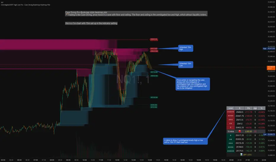
Dragon Flow Arrows (LITE)🚀 DRAGON FLOW ARROWS — LITE | Smart Trend Engine + Clean Reversal Arrows
A lightweight but highly-optimized trend system designed for clean charts, powerful visual signals, and no-noise directional flow.
Built for traders who want simplicity, clarity, and professional-level momentum-filtered signals without over-complication.
🔥 Dragon Channel (Clean 3-Line Ribbon)
A smooth adaptive channel formed from ATR + EMA, giving you structural trend zones without clutter.
✅ Dragon Flow Gradient
A horizontal, color-shifted flow:
🟢 Bull flow → green glow
🔴 Bear flow → red glow
Automatic blend based on trend direction
Smooth visual transitions (no vertical stripes)
✅ Momentum-Filtered Arrows (No Spam)
BUY/SELL arrows only print when:
Price breaks outside the Dragon Channel
Momentum confirms (RSI + MACD filters)
Trend flips → one clean arrow per direction
Text labels sit outside the channel for better readability.
✅ Smart Header Panel
At the top of your chart:
📌 Trend: Uptrend / Downtrend / Neutral
⚡ Impulse Strength: Weak / Normal / Strong
📊 How to Use
Entry:
BUY Setup
Price moving above baseline
Dragon Flow turns bullish (cyan side)
Arrow appears below channel
SELL Setup
Price breaks below baseline
Dragon Flow turns bearish (magenta side)
Arrow pops above channel
Exit / Filter:
Opposite arrow
Flow color shift
Trend panel flips
Works on Forex, Crypto, Stocks, Indices — all timeframes.
Happy trading!

Algorithmic Volume Rejection Zones [AVRZ]Hello traders,
I am pleased to release the Algorithmic Volume Rejection Zones (AVRZ). This is a specialized decision-support system designed to identify high-probability reversal points by synthesizing candle geometry, market structure, and statistical volume anomalies.
Trading reversals often presents a dilemma: wait for confirmation and miss the move, or enter early and get stopped out by noise. AVRZ solves this by quantifying "Institutional Absorption." It filters out weak price probes and highlights only the specific moments where significant volume has stepped in to defend a price level.
🛡️ The Concept: Attacking The Zonesl
You will often see price aggressively "attack" a support or resistance level with speed and high volume. To the untrained eye, this looks like a breakout. However, professional analysis reveals that this is often an Efficiency Event—liquidity is being absorbed by passive limit orders.
The AVRZ indicator is specifically engineered to detect this phenomenon. When price strikes a level and volume spikes (>2.0 Sigma), it signals that the auction is becoming efficient and a reversal is imminent. The script captures this "Attack" via the Climax Bypass logic, plotting a fresh zone immediately to mark where the liquidity was defended.

TuxAlgo Plus a SMC and Trap Toolkit V0.98r1 by McTogaThe “TuxAlgo Plus” script is a powerful, standalone, conceptual open-source project and self-sufficient “smart money toolkit” with automatic trap detection (SMT), liquidity grabs, FVG confluence, and complete bot setup signals for TV charts in the “H1 to H6” time frame and daily charts.
The script is used to improve SMC/trap analyses, i.e., the structure and visualization logic for TradingView charts have been expanded in the “TuxAlgo++” project in line with Smart Money Concepts (SMC) and Smart Money Traps (SMT).
The SMT block (“Smart Money Traps”) supplements classic smart money concepts with:
1. Detection of bull traps (short setups) and bear traps (long setups)
2. Display of trap boxes in the chart (liquidity grab areas)
3. A bot setup box (table) with ready-made entry/SL/TP levels:
as well as age in bars & days and “Valid until ~X d” (remaining term)
SMT / bot setup only run on the following timeframes:
- H1, H2, H3, H4, H6 This means that traps, labels, and the bot setup box are only displayed on these timeframes
Trap definition “Bull Trap (Short Setup)”:
- Valid swing high
- Swing trend bullish
- High (Wick) pierces above the swing high (Liquidity Grab)
- Close falls back below the swing high (false breakout)
-> Result: Short setup (bull trap), marked in orange
Trap definition “Bear Trap (long setup)”:
- Valid swing low
- Swing trend bearish
- Low (wick) pierces below the swing low (liquidity grab)
- Close rises above the swing low again (false breakout)
-> Result: Long setup (bear trap), marked in blue
Entry / SL / TP calculation
A price range is taken for each trap:
Bull trap (short):
- Range =
- Entry = point within this range:
Entry = hiBT - (hiBT - loBT) * TrapEntryRatio (0..1)
-> 0.0 = at the Wick extreme, 0.5 = middle, 1.0 = at the Swing level
- SL = Wick extreme (upper edge of the trap)
- Risk = |Entry - SL|
- TP1 = Entry - R1 * Risk
- TP2 = Entry - R2 * Risk
Bear Trap (Long):
- Range =
- Entry analogous within the range according to TrapEntryRatio
- SL = wick bottom (lower edge of the trap)
- Risk = |Entry - SL|
- TP1 = Entry + R1 * Risk
- TP2 = Entry + R2 * Risk
R1 / R2 correspond to the inputs:
- botRR1Input = TP1 Risk/Reward (e.g., 1.5R)
- botRR2Input = TP2 Risk/Reward (e.g., 3.0R)
Age & Validity
Each trap stores:
- lastTrapBarIndex -> last bar of the trap
- Age in bars -> bar_index - lastTrapBarIndex
- Age in days (~d) -> AgeBars * BarDurationInDays (depending on TF)
Input: trapMaxAgeBars determines how long a trap is valid.
The bot setup box is only displayed if:
- a trap is present,
- AgeBars <= trapMaxAgeBars,
- SMT + Box + SMC timeframe are active.
Color logic (color blind friendly):
- Blue (accentBlue) = fresh traps (Age <= 1/3 MaxAge)
- Orange (accentOrange) = medium age
- Violet (accentPurple) = old, but still within MaxAge
- Gray (accentGray) = expired (> MaxAge)
The box also shows “Valid until ~X d” as the remaining term.
Day/Night Mode & Colors
- chart.bg_color is used to detect dark or light mode.
- Text/background colors adjust (light/dark).
- Accent colors (blue/orange/purple/gray) are suitable for red/green color blindness.
- Trap labels in the chart:
- Bull trap label = orange (short setup)
- Bear trap label = blue (long setup)
- Text color depends on chart mode (dark/light)
Typical workflow (example):
1. Select a suitable symbol & SMC timeframe (e.g., H4 or H6).
2. Wait for a bull trap (short) or bear trap (long).
3. Read in the bot setup box:
- Direction (long/short)
- Entry, SL, TP1, TP2
- Age & “Valid until ~X d”
4. These values can be used as a template for manual trading or external bot/order systems.
5. Position size & leverage must always be calculated separately in your own risk management
(e.g., 2% rule). This script does not calculate position sizes.

Open Interest Bubbles [BackQuant]Open Interest Bubbles
A visual OI positioning overlay that aggregates futures open interest across major venues, normalizes it into a consistent “signal strength” scale, then plots extreme events as bubbles, labels, and optional horizontal levels directly on price.
What this is for
Open interest is one of the cleanest ways to track when positioning is building, unwinding, or aggressively shifting. The problem is raw OI is noisy, exchange-specific, and hard to compare across time. This script solves that by:
- Aggregating OI across multiple exchanges.
- Letting you choose what “OI signal” you care about (raw, delta, percent versions).
- Normalizing the signal so “big events” are easy to spot.
- Plotting those events as bubbles and levels at the exact price they occurred.
You end up with a clean, fast visual map of where large positioning changes occurred, and where those events may later matter as reaction points.
────────────────────────────────────────────────────────────
Plotting types (what you can display)
Bubbles
This mode plots OI events as size-bucketed circles on the chart. Bigger bubbles represent stronger normalized events. You can tune:
- Bubble sizing by bucket (Tiny → Huge).
- Heatmap vs solid color styling.
- Signed vs unsigned coloring (positive/negative separation or magnitude-only).
Best use:
- Spotting “where something changed” at a glance.
- Identifying clusters of positioning events around key price zones.
- Seeing whether the market is repeatedly building/closing positions at similar levels.
Levels
Levels mode draws a horizontal line at the anchor price when an extreme OI event triggers. These act like “positioning memory” levels:
- They do not claim to be support/resistance by themselves.
- They highlight prices where the derivatives market clearly did something meaningful.
Best use:
- Marking potential reaction zones.
- Combining with your price action tools (structure, OBs, FVGs) to confirm whether an OI level aligns with a technical level.
- Building a “map” of where leverage likely entered or exited.
Modes available in the script:
- Off
- Bubbles
- Bubbles + Labels
- Labels Only
- Levels + Labels
────────────────────────────────────────────────────────────
Aggregated Open Interest source (multi-exchange)
This indicator builds a single aggregated OI series by requesting OI data from multiple exchanges and summing it. You can toggle exchanges on/off:
- Binance, Bybit, OKX, Bitget, Kraken, HTX, Deribit
You can also choose OI units:
- COIN , OI in base units (native sizing)
- USD , converted for a dollar-value representation
Important note:
Not every symbol has OI data on every venue. If the script cannot build an aggregated series for the symbol, it will throw an error rather than quietly plotting garbage.
────────────────────────────────────────────────────────────
OI Source, what the bubbles are measuring
You control what “signal” is normalized and plotted:
- Delta , change in aggregated OI from the prior bar.
Use when you want to highlight bursts of new positioning or sudden unwind events.
- Raw OI , the aggregated open interest level itself.
Use when you want to highlight absolute positioning build-up periods.
- Delta % , percent change in OI.
Use when you want moves normalized to the current OI regime, useful across different market eras.
- Raw OI % , percent change form of the raw series.
Use when you want relative changes rather than absolute size.
Practical guidance:
- Delta modes are best for “event detection”.
- Raw modes are better for “regime context” and whether positioning is structurally rising or fading.
────────────────────────────────────────────────────────────
Normalization (the key to making it readable)
Because OI varies massively across assets and time, the script includes multiple normalization modes to convert your chosen OI source into a comparable “strength” value.
Options:
- ZScore , deviation from a rolling mean in standard deviation units.
- StdNorm , scaled by rolling standard deviation.
- AbsZScore , absolute value version for magnitude-only mapping.
- AbsStdNorm , absolute value version for magnitude-only mapping.
- None , plots raw values (advanced users only, often too noisy visually).
Why this matters:
Normalization makes a “1.5” or “3.0” threshold mean something across different assets and timeframes, instead of being stuck to raw OI units.
────────────────────────────────────────────────────────────
Threshold system (when bubbles/levels trigger)
The plot is driven by two user thresholds:
- Base Threshold
Controls where “meaningful” events start. Raising this reduces noise and focuses on larger deviations.
- Extreme Threshold
Controls what qualifies as a top-tier event. Extreme events are what you typically want to convert into labels and levels.
You also control side filtering:
- Both , show positive and negative events.
- Positive Only , show only increases (or positive signal side depending on source).
- Negative Only , show only decreases (or negative signal side).
In practice:
- Use Base Threshold to tune chart cleanliness.
- Use Extreme Threshold to mark only the “big stuff” that tends to matter later.
────────────────────────────────────────────────────────────
Anchor Source (where the bubble/level is placed)
The indicator places bubbles, labels, and levels at a price anchor you choose:
- HL2, Close, Open, High, Low, VWAP
This is important because “where you pin the event” changes how it reads:
- Close is clean and consistent for backtesting and candle-close logic.
- High/Low can better represent where the fight occurred intrabar.
- VWAP can be useful for “fair price” anchoring in active markets.
────────────────────────────────────────────────────────────
Style system (theme, palette, signed logic)
This script is built to look good and stay readable on busy charts.
Themes
- BackQuant, Classic, Ice, Fire, Mono, Custom
Palette Mode
- Solid , one consistent color
- Heatmap , intensity increases with magnitude
- Single Color Adaptive , adapts to chart background for clarity
Side Coloring
- Signed , positive and negative events can use different ramps
- Unsigned , magnitude-only coloring
Negative theme handling:
- Auto (mirrors your chosen theme),
- Invert (flips the ramp),
- Custom (fully user-defined negative palette).
What this gives you:
- You can run a clean “mono” look for professional charts.
- Or a high-contrast heatmap for fast scanning.
- Or fully custom branding colors for BackQuant-style presentation.
────────────────────────────────────────────────────────────
Labels (what’s inside the label)
When labels are enabled, the script can display:
- OI , the aggregated OI value
- OI + Norm , OI plus normalized strength
- Norm Only , just the normalized strength
- Src + Norm , the selected source value (Delta, Raw, %) plus normalized strength
You can also control:
- Left/Center/Right label alignment
- Number formatting style (Raw, Compact, Volume format)
Best practice:
- Use “Src + Norm” when you want both the raw event size and its rarity.
- Use “Norm Only” when you want a clean, minimal chart.
────────────────────────────────────────────────────────────
Levels and object limits (performance and cleanliness)
Because this script draws objects, it includes a hard cleanup system:
- You set Max Levels / Labels to control chart clutter.
- The script deletes older lines/labels when the limit is exceeded.
This is critical if you trade lower timeframes, where OI events can trigger frequently.
────────────────────────────────────────────────────────────
How to interpret the signals
What a large bubble usually means:
- A statistically large positioning change relative to recent history.
- This can represent fresh leverage entering, forced liquidations, or aggressive de-risking, depending on direction and context.
How to use levels:
- Treat them as “attention levels”, not automatic entries.
- Combine them with structure and liquidity tools:
- If price revisits an OI level and shows rejection, it often confirms that level mattered.
- If price slices through with no reaction, it often indicates the OI event was transitional, not defended.
Common setups:
- Clustered extreme bubbles near a breakout zone, then retest later.
- Extreme negative event at capitulation low, followed by structure flip.
- Extreme positive build into resistance, then unwind and mean reversion.
Also, please check out @NoveltyTrade for the OI Aggregation logic & pulling the data source!
Here is the original script:
