STD-Filtered, Variety FIR Digital Filters w/ ATR Bands [Loxx]STD-Filtered, Variety FIR Digital Filters w/ ATR Bands is a FIR Digital Filter indicator with ATR bands. This indicator contains 12 different digital filters. Some of these have already been covered by indicators that I've recently posted. The difference here is that this indicator has ATR bands, allows for frequency filtering, adds a frequency multiplier, and attempts show causality by lagging price input by 1/2 the period input during final application of weights. Period is restricted to even numbers.
The 3 most important parameters are the frequency cutoff, the filter window type and the "causal" parameter.
Included filter types:
- Hamming
- Hanning
- Blackman
- Blackman Harris
- Blackman Nutall
- Nutall
- Bartlet Zero End Points
- Bartlet Hann
- Hann
- Sine
- Lanczos
- Flat Top
Frequency cutoff can vary between 0 and 0.5. General rule is that the greater the cutoff is the "faster" the filter is, and the smaller the cutoff is the smoother the filter is.
You can read more about discrete-time signal processing and some of the windowing functions in this indicator here:
Window function
Window Functions and Their Applications in Signal Processing
What are FIR Filters?
In discrete-time signal processing, windowing is a preliminary signal shaping technique, usually applied to improve the appearance and usefulness of a subsequent Discrete Fourier Transform. Several window functions can be defined, based on a constant (rectangular window), B-splines, other polynomials, sinusoids, cosine-sums, adjustable, hybrid, and other types. The windowing operation consists of multipying the given sampled signal by the window function. For trading purposes, these FIR filters act as advanced weighted moving averages.
A finite impulse response (FIR) filter is a filter whose impulse response (or response to any finite length input) is of finite duration, because it settles to zero in finite time. This is in contrast to infinite impulse response (IIR) filters, which may have internal feedback and may continue to respond indefinitely (usually decaying).
The impulse response (that is, the output in response to a Kronecker delta input) of an Nth-order discrete-time FIR filter lasts exactly {\displaystyle N+1}N+1 samples (from first nonzero element through last nonzero element) before it then settles to zero.
FIR filters can be discrete-time or continuous-time, and digital or analog.
A FIR filter is (similar to, or) just a weighted moving average filter, where (unlike a typical equally weighted moving average filter) the weights of each delay tap are not constrained to be identical or even of the same sign. By changing various values in the array of weights (the impulse response, or time shifted and sampled version of the same), the frequency response of a FIR filter can be completely changed.
An FIR filter simply CONVOLVES the input time series (price data) with its IMPULSE RESPONSE. The impulse response is just a set of weights (or "coefficients") that multiply each data point. Then you just add up all the products and divide by the sum of the weights and that is it; e.g., for a 10-bar SMA you just add up 10 bars of price data (each multiplied by 1) and divide by 10. For a weighted-MA you add up the product of the price data with triangular-number weights and divide by the total weight.
What is a Standard Deviation Filter?
If price or output or both don't move more than the (standard deviation) * multiplier then the trend stays the previous bar trend. This will appear on the chart as "stepping" of the moving average line. This works similar to Super Trend or Parabolic SAR but is a more naive technique of filtering.
Included
Bar coloring
Loxx's Expanded Source Types
Signals
Alerts
Related indicators
STD/C-Filtered, N-Order Power-of-Cosine FIR Filter
STD/C-Filtered, Power-of-Cosine FIR Filter
STD/C-Filtered, Truncated Taylor Family FIR Filter
STD/Clutter-Filtered, Variety FIR Filters
STD/Clutter-Filtered, Kaiser Window FIR Digital Filter
"如何用wind搜索股票的发行价和份数"に関するスクリプトを検索
Stock WatchOverview
Watch list are very common in trading, but most of them simply provide the means of tracking a list of symbols and their current price. Then, you click through the list and perform some additional analysis individually from a chart setup. What this indicator is designed to do is provide a watch list that employs a high/low price range analysis in a table view across multiple time ranges for a much faster analysis of the symbols you are watching.
Discussion
The concept of this Stock Watch indicator is best understood when you think in terms of a 52 Week Range indication on many financial web sites. Taken a given symbol, what is the high and the low over a 52 week range and then determine where current price is within that range from a percentage perspective between 0% and 100%.
With this concept in mind, let's see how this Stock Watch indicator is meant to benefit.
There are four different H/L ranges relative to the chart's setting and a Scope property. Let's use a three month (3M) chart as our example and set the indicator's Scope = 4. A 3M chart provides three months of data in a single candle, now when we set the Scope = 4 we are stating that 1X is going to look over four candles for the high/low range.
The Scope property is used to determine how many candles it is to scan to determine the high/low range for the corresponding 1X, 3X, 5X and 10X periods. This is how different time ranges are put into perspective. Using a 3M chart with Scope = 4 would represent the following time windows:
- 1X = 3M * 4 is a 12 Months or 1 Year High/Low Range
- 3X = 3M * 4 * 3 is a 36 Months or 3 Years High/Low Range
- 5X = 3M * 4 * 5 is a 60 Months or 5 Years High/Low Range
- 10X = 3M * 4 * 10 is a 120 Months or 10 Years High/Low Range.
With these calculations, the indicator then determines where current price is within each of these High/Low ranges from a percentage perspective between 0% and 100%.
Once the 0% to 100% value is calculated, it then will shade the value according to a color gradient from red to green (or any other two colors you set the indictor to). This color shading really helps to interpret current price quickly.
The greater power to this range and color shading comes when you are able to see where price is according to price history across the multiple time windows. In this example, there is quick analysis across 1 Year, 3 Year, 5 Year and 10 Year windows.
Now let's further improve this quick analysis over 15 different stocks for which the indicator allows you to watch up to at any one time.
For value traders this is huge, because we're always looking for the bargains and we wait for price to be in the value range. Using this indicator helps to instantly see if price has entered a value range before we decide to do further analysis with other charting and fundamental tools.
The Code
The heart of all this is really very simple as you can see in the following code snippet. We're simply looking for the highest high and lowest low across the different scopes and calculating the percentage of the range where current price is for each symbol being watched.
scope = baseScope
watch1X = math.round(((watchClose - ta.lowest(watchLow, scope)) / (ta.highest(watchHigh, scope) - ta.lowest(watchLow, scope))) * 100, 0)
table.cell(tblWatch, columnId, 2, str.format("{0, number, #}%", watch1X), text_size = size.small, text_color = colorText, bgcolor = getBackColor(watch1X))
//3X Lookback
scope := baseScope * 3
watch3X = math.round(((watchClose - ta.lowest(watchLow, scope)) / (ta.highest(watchHigh, scope) - ta.lowest(watchLow, scope))) * 100, 0)
table.cell(tblWatch, columnId, 3, str.format("{0, number, #}%", watch3X), text_size = size.small, text_color = colorText, bgcolor = getBackColor(watch3X))
Conclusion
The example I've laid out here are for large time windows, because I'm a long term investor. However, keep in mind that this can work on any chart setting, you just need to remember that your chart's time period and scope work together to determine what 1X, 3X, 5X and 10X represent.
Let me try and give you one last scenario on this. Consider your chart is set for a 60 minute chart, meaning each candle represents 60 minutes of time and you set the Stock Watch indicator to a scope = 4. These settings would now represent the following and you would be watching up to 15 different stocks across these windows at one time.
1X = 60 minutes * 4 is 240 minutes or 4 hours of time.
3X = 60 minutes * 4 * 3 = 720 minutes or 12 hours of time.
5X = 60 minutes * 4 * 5 = 1200 minutes or 20 hours of time.
10X = 60 minutes * 4 * 10 = 2400 minutes or 40 hours of time.
I hope you find value in my contribution to the cause of trading, and if you have any comments or critiques, I would love to here from you in the comments.

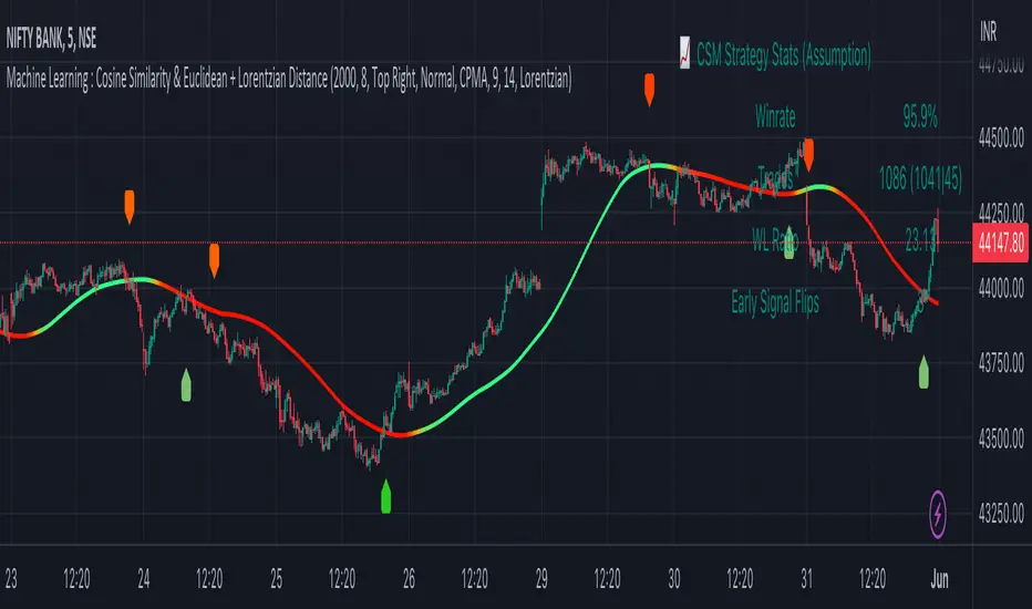
Machine Learning : Cosine Similarity & Euclidean DistanceIntroduction:
This script implements a comprehensive trading strategy that adheres to the established rules and guidelines of housing trading. It leverages advanced machine learning techniques and incorporates customised moving averages, including the Conceptive Price Moving Average (CPMA), to provide accurate signals for informed trading decisions in the housing market. Additionally, signal processing techniques such as Lorentzian, Euclidean distance, Cosine similarity, Know sure thing, Rational Quadratic, and sigmoid transformation are utilised to enhance the signal quality and improve trading accuracy.
Features:
Market Analysis: The script utilizes advanced machine learning methods such as Lorentzian, Euclidean distance, and Cosine similarity to analyse market conditions. These techniques measure the similarity and distance between data points, enabling more precise signal identification and enhancing trading decisions.
Cosine similarity:
Cosine similarity is a measure used to determine the similarity between two vectors, typically in a high-dimensional space. It calculates the cosine of the angle between the vectors, indicating the degree of similarity or dissimilarity.
In the context of trading or signal processing, cosine similarity can be employed to compare the similarity between different data points or signals. The vectors in this case represent the numerical representations of the data points or signals.
Cosine similarity ranges from -1 to 1, with 1 indicating perfect similarity, 0 indicating no similarity, and -1 indicating perfect dissimilarity. A higher cosine similarity value suggests a closer match between the vectors, implying that the signals or data points share similar characteristics.
Lorentzian Classification:
Lorentzian classification is a machine learning algorithm used for classification tasks. It is based on the Lorentzian distance metric, which measures the similarity or dissimilarity between two data points. The Lorentzian distance takes into account the shape of the data distribution and can handle outliers better than other distance metrics.
Euclidean Distance:
Euclidean distance is a distance metric widely used in mathematics and machine learning. It calculates the straight-line distance between two points in Euclidean space. In two-dimensional space, the Euclidean distance between two points (x1, y1) and (x2, y2) is calculated using the formula sqrt((x2 - x1)^2 + (y2 - y1)^2).
Dynamic Time Windows: The script incorporates a dynamic time window function that allows users to define specific time ranges for trading. It checks if the current time falls within the specified window to execute the relevant trading signals.
Custom Moving Averages: The script includes the CPMA, a powerful moving average calculation. Unlike traditional moving averages, the CPMA provides improved support and resistance levels by considering multiple price types and employing a combination of Exponential Moving Averages (EMAs) and Simple Moving Averages (SMAs). Its adaptive nature ensures responsiveness to changes in price trends.
Signal Processing Techniques: The script applies signal processing techniques such as Know sure thing, Rational Quadratic, and sigmoid transformation to enhance the quality of the generated signals. These techniques improve the accuracy and reliability of the trading signals, aiding in making well-informed trading decisions.
Trade Statistics and Metrics: The script provides comprehensive trade statistics and metrics, including total wins, losses, win rate, win-loss ratio, and early signal flips. These metrics offer valuable insights into the performance and effectiveness of the trading strategy.
Usage:
Configuring Time Windows: Users can customize the time windows by specifying the start and finish time ranges according to their trading preferences and local market conditions.
Signal Interpretation: The script generates long and short signals based on the analysis, custom moving averages, and signal processing techniques. Users should pay attention to these signals and take appropriate action, such as entering or exiting trades, depending on their trading strategies.
Trade Statistics: The script continuously tracks and updates trade statistics, providing users with a clear overview of their trading performance. These statistics help users assess the effectiveness of the strategy and make informed decisions.
Conclusion:
With its adherence to housing trading rules, advanced machine learning methods, customized moving averages like the CPMA, and signal processing techniques such as Lorentzian, Euclidean distance, Cosine similarity, Know sure thing, Rational Quadratic, and sigmoid transformation, this script offers users a powerful tool for housing market analysis and trading. By leveraging the provided signals, time windows, and trade statistics, users can enhance their trading strategies and improve their overall trading performance.
Disclaimer:
Please note that while this script incorporates established tradingview housing rules, advanced machine learning techniques, customized moving averages, and signal processing techniques, it should be used for informational purposes only. Users are advised to conduct their own analysis and exercise caution when making trading decisions. The script's performance may vary based on market conditions, user settings, and the accuracy of the machine learning methods and signal processing techniques. The trading platform and developers are not responsible for any financial losses incurred while using this script.
By publishing this script on the platform, traders can benefit from its professional presentation, clear instructions, and the utilisation of advanced machine learning techniques, customised moving averages, and signal processing techniques for enhanced trading signals and accuracy.
I extend my gratitude to TradingView, LUX ALGO, and JDEHORTY for their invaluable contributions to the trading community. Their innovative scripts, meticulous coding patterns, and insightful ideas have profoundly enriched traders' strategies, including my own.
JOPA Channel (Dual-Volumed) v1 [JopAlgo]JOPA Channel (Dual-Volumed) v1
Short title: JOPAV1 • License: MPL-2.0 • Provider: JopAlgo
We have developed our own, first channel-based trading indicator and we’re making it available to all traders. The goal was a channel that breathes with the tape—built on a volume-weighted backbone—so the outcome stays lively instead of static. That led to the JOPA Channel.
All important features (at a glance)
In one line: A Rolling-VWAP channel whose width adapts with two volumes (RVOL + dollar-flow), adds order-flow asymmetry (OBV tilt) and regime awareness (Efficiency Ratio), and frames risk with outer containment bands from residual extremes—so you see fair value, momentum, and exhaustion in one view.
Feature list
Rolling VWAP centerline: Tracks where volume traded (fair value).
Dual-volume width: Bands expand/contract with relative volume and value traded (price×volume).
OBV tilt: Upper/lower widths skew toward the side actually pushing.
Regime adapter (ER): Tighter in trend, wider in chop—automatically.
Outer containment rails: Residual-extreme ceilings/floors, smoothed + margin.
20% / 80% guides: 20% light blue (discount), 80% light red (premium).
Squeeze dots (optional): Orange circles below candles during compression.
Non-repainting: Uses rolling sums and past-only math; no lookahead.
Default visual in this release
Containment rails + fill: ON (stepline, medium).
Inner Value rails + fill: Rails OFF (stepline, thin), fill ON (drawn only if rails are shown).
20% & 80% guides: ON (dashed, thin; 20% light blue, 80% light red).
Squeeze dots: OFF by default (orange circles when enabled).
What you see on the chart
RVWAP (centerline): Your compass for fair value.
Inner Value Bands (optional): Tight rails for breakouts and pullback timing.
Outer Containment Bands (default ON): High-confidence ceilings/floors for targets and fades.
20% / 80% guides: Quick read of “where in the channel” price is sitting.
Squeeze dots (optional): Volatility compression heads-up (no text labels).
Non-repainting note: The indicator does not revise closed bars. Forecast-Lock uses linear regression to extrapolate 1–3 bars ahead without using future data.
How to use it
Core reads (works on any timeframe)
Bias: Above a rising RVWAP → long bias; below a falling RVWAP → short bias.
Breakouts (momentum): Close beyond an Inner Value rail with RVOL ≥ threshold (alert provided).
Reversions (fades): Tag Outer Containment, stall, then close back inside → expect mean reversion toward RVWAP.
20/80 timing:
At/above 80% (light red) → premium/exhaustion risk; trim longs or consider fades if RVOL cools.
At/below 20% (light blue) → discount/exhaustion risk; trim shorts or consider longs if RVOL cools.
Squeeze clusters: When dots bunch up, expect a range break; use the Breakout alert as confirmation.
Playbooks by trading style
Day Trading (1–5m)
Setup: Keep the chart clean (Containment ON, Value rails OFF). Toggle Inner Value ON when hunting a breakout or timing a pullback.
Pullback Long: Dip to RVWAP / Lower Value with sub-threshold RVOL, then a close back above RVWAP → long.
Stop: Just beyond Lower Containment or the pullback swing.
Targets (1:1:1): ⅓ at RVWAP, ⅓ at Upper Value, ⅓ trail toward Upper Containment.
Breakout Long: After a squeeze cluster, take the Breakout Long alert (close > Upper Value, RVOL ≥ min). If no retest, demand the next bar holds outside.
Range Fade: Only when RVWAP is flat and dots cluster; short Upper Containment → RVWAP (mirror for longs at the lower rail).
Intraday (15m–1H)
HTF compass: Take bias from 4H.
Pullback Long: “Touch & reclaim” of RVWAP while RVOL cools; enter on the reclaim close or break of that candle’s high.
Breakout: Run Inner Value ON; act on Breakout alerts (RVOL gate ≈ 1.10–1.15 typical).
Avoid low-probability fades against the 4H slope unless RVWAP is flat.
Swing (4H–1D)
Continuation: In uptrends, buy pullbacks to RVWAP / Lower Value with sub-threshold RVOL; scale at Upper Containment.
Adds: Post-squeeze Breakout Long adds; trail on RVWAP or Lower Value.
Fades: Prefer when RVWAP flattens and price oscillates between containments.
Position (1D+)
Framework: Daily RVWAP slope + position within containment.
Add rule: Each reclaim of RVWAP after a dip is an add; trim into Upper Containment or near 80% light red.
Sizing: Containment distance is larger—size down and trail on RVWAP.
Inputs & Settings (complete)
Core
Source: Price input for RVWAP.
Rolling VWAP Length: Window of the centerline (higher = smoother).
Volume Baseline (RVOL): SMA window for relative volume.
Inner Value Bands (volatility-based width)
k·StdDev(residuals), k·ATR, k·MAD(residuals): Blend three measures into base width.
StdDev / ATR / MAD Lengths: Lookbacks for each.
Two-Volume Fusion
RVOL Exponent: How aggressively width responds to relative volume.
Dollar-Flow Gain: Adds push from price×volume (value traded).
Dollar-Flow Z-Window: Standardization window for dollar-flow.
Asymmetry (Order-Flow Tilt)
Enable Tilt (OBV): Lets flow skew upper/lower widths.
Tilt Strength (0..1): Gain applied to OBV slope z-score.
OBV Slope Z-Window: Window to standardize OBV slope.
Regime Adapter
Efficiency Ratio Lookback: Measures trend vs chop.
ER Width Min/Max: Maps ER into a width factor (tighter in trend, wider in chop).
Band Tracking (inner value rails)
Tracking Mode:
Base: Pure base rails.
Parallel-Lock: Smooth RVWAP & width; track in parallel.
Slope-Lock: Adds a fraction of recent slope (momentum-friendly).
Forecast-Lock: 1–3 bar extrapolation via linreg (non-repainting on closed bars).
Attach Strength (0..1): Blend tracked rails vs base rails.
Tracking Smooth Length: EMA smoothing of RVWAP and width.
Slope Influence / Forecast Lead Bars: Gains for the chosen mode.
Outer Containment Bands
Show Containment Bands: Master toggle (default ON).
Residual Extremes Lookback: Highest/lowest residual window.
Extreme Smoothing (EMA): Stability on extreme lines.
Margin vs inner width: Extra padding relative to smoothed inner width.
Squeeze & Alerts
Squeeze Window / Threshold: Width vs average; at/under threshold = dot (when enabled).
Min RVOL for Breakout: Required RVOL for breakout alerts.
Style (defaults in this release)
Inner Value rails: OFF (stepline, thin).
Inner & Containment fills: ON.
Containment rails: ON (stepline, medium).
20% / 80% guides: ON — 20% light blue, 80% light red, dashed, thin.
Squeeze dots: OFF by default (orange circles below candles when enabled).
Practical templates (copy/paste into a plan)
Momentum Breakout
Context: Squeeze cluster near RVWAP; Inner Value ON.
Trigger: Breakout Long (close > Upper Value & RVOL ≥ min).
Stop: Below Lower Value (tight) or below RVWAP (safer).
Targets (1:1:1): ⅓ Value → ⅓ Containment → ⅓ trail on RVWAP.
Pullback Continuation
Context: Uptrend; dip to RVWAP / Lower Value with cooling RVOL.
Trigger: Close back above RVWAP or break of reclaim candle’s high.
Stop: Just outside Lower Containment or pullback swing.
Targets: RVWAP → Upper Value → Upper Containment.
Containment Reversion (range)
Context: RVWAP flat; repeated containment tags.
Trigger: Stall at containment, then close back inside.
Stop: A step beyond that containment.
Target: RVWAP; runner only if RVOL stays muted.
Alerts included
DVWAP Breakout Long / Short (Value Bands)
Top Zone / Bottom Zone (20% / 80% guides)
Tip: On lower TFs, act on Breakout alerts with higher-TF bias (e.g., trade 5–15m in the direction of 1H/4H RVWAP slope/position).
Best practices
Let RVWAP be the compass; if unsure, wait until price picks a side.
Respect RVOL; low-RVOL breaks are prone to fail.
Use guides for timing, not certainty. Pair 20/80 zones with flow context.
Start with defaults; change one knob at a time.
Common pitfalls
Fading every containment touch → only fade when RVWAP is flat or RVOL cools.
Over-tuning inputs → the defaults are robust; small tweaks go a long way.
Fighting the higher timeframe on low TFs → expensive habit.
Footer — License & Publishing
License: Mozilla Public License 2.0 (MPL-2.0). You may modify and redistribute; keep this file under MPL and provide source for this file.
Originality: © 2025 JopAlgo. No third-party code reused; Pine built-ins and common formulas only.
Publishing: Keep this header/description intact when releasing on TradingView. Avoid promotional links in the public script text.

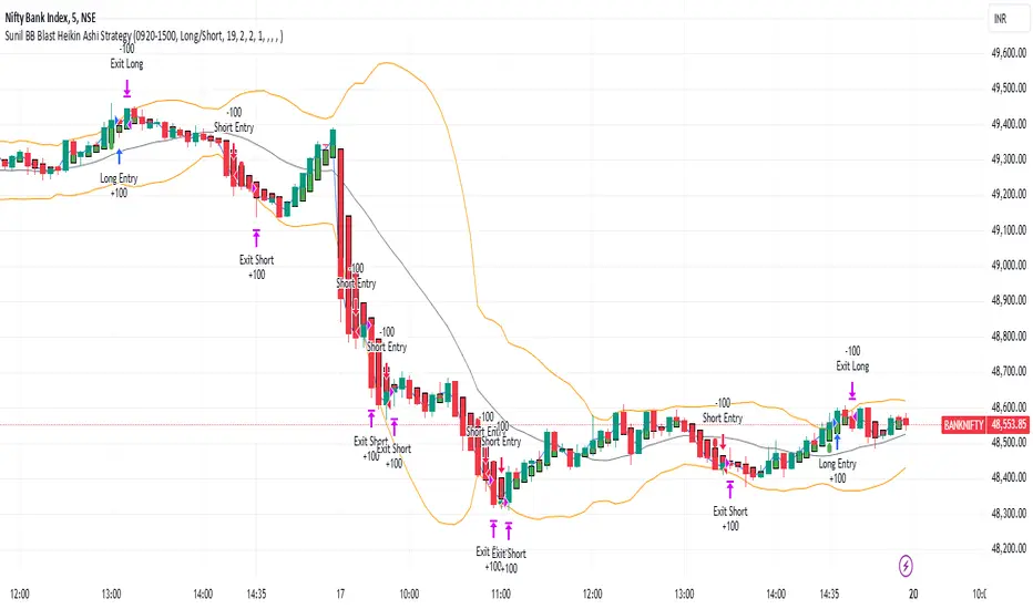
Sunil BB Blast Heikin Ashi StrategySunil BB Blast Heikin Ashi Strategy
The Sunil BB Blast Heikin Ashi Strategy is a trend-following trading strategy that combines Bollinger Bands with Heikin-Ashi candles for precise market entries and exits. It aims to capitalize on price volatility while ensuring controlled risk through dynamic stop-loss and take-profit levels based on a user-defined Risk-to-Reward Ratio (RRR).
Key Features:
Trading Window:
The strategy operates within a user-defined time window (e.g., from 09:20 to 15:00) to align with market hours or other preferred trading sessions.
Trade Direction:
Users can select between Long Only, Short Only, or Long/Short trade directions, allowing flexibility depending on market conditions.
Bollinger Bands:
Bollinger Bands are used to identify potential breakout or breakdown zones. The strategy enters trades when price breaks through the upper or lower Bollinger Band, indicating a possible trend continuation.
Heikin-Ashi Candles:
Heikin-Ashi candles help smooth price action and filter out market noise. The strategy uses these candles to confirm trend direction and improve entry accuracy.
Risk Management (Risk-to-Reward Ratio):
The strategy automatically adjusts the take-profit (TP) level and stop-loss (SL) based on the selected Risk-to-Reward Ratio (RRR). This ensures that trades are risk-managed effectively.
Automated Alerts and Webhooks:
The strategy includes automated alerts for trade entries and exits. Users can set up JSON webhooks for external execution or trading automation.
Active Position Tracking:
The strategy tracks whether there is an active position (long or short) and only exits when price hits the pre-defined SL or TP levels.
Exit Conditions:
The strategy exits positions when either the take-profit (TP) or stop-loss (SL) levels are hit, ensuring risk management is adhered to.
Default Settings:
Trading Window:
09:20-15:00
This setting confines the strategy to the specified hours, ensuring trading only occurs during active market hours.
Strategy Direction:
Default: Long/Short
This allows for both long and short trades depending on market conditions. You can select "Long Only" or "Short Only" if you prefer to trade in one direction.
Bollinger Band Length (bbLength):
Default: 19
Length of the moving average used to calculate the Bollinger Bands.
Bollinger Band Multiplier (bbMultiplier):
Default: 2.0
Multiplier used to calculate the upper and lower bands. A higher multiplier increases the width of the bands, leading to fewer but more significant trades.
Take Profit Multiplier (tpMultiplier):
Default: 2.0
Multiplier used to determine the take-profit level based on the calculated stop-loss. This ensures that the profit target aligns with the selected Risk-to-Reward Ratio.
Risk-to-Reward Ratio (RRR):
Default: 1.0
The ratio used to calculate the take-profit relative to the stop-loss. A higher RRR means larger profit targets.
Trade Automation (JSON Webhooks):
Allows for integration with external systems for automated execution:
Long Entry JSON: Customizable entry condition for long positions.
Long Exit JSON: Customizable exit condition for long positions.
Short Entry JSON: Customizable entry condition for short positions.
Short Exit JSON: Customizable exit condition for short positions.
Entry Logic:
Long Entry:
The strategy enters a long position when:
The Heikin-Ashi candle shows a bullish trend (green close > open).
The price is above the upper Bollinger Band, signaling a breakout.
The previous candle also closed higher than it opened.
Short Entry:
The strategy enters a short position when:
The Heikin-Ashi candle shows a bearish trend (red close < open).
The price is below the lower Bollinger Band, signaling a breakdown.
The previous candle also closed lower than it opened.
Exit Logic:
Take-Profit (TP):
The take-profit level is calculated as a multiple of the distance between the entry price and the stop-loss level, determined by the selected Risk-to-Reward Ratio (RRR).
Stop-Loss (SL):
The stop-loss is placed at the opposite Bollinger Band level (lower for long positions, upper for short positions).
Exit Trigger:
The strategy exits a trade when either the take-profit or stop-loss level is hit.
Plotting and Visuals:
The Heikin-Ashi candles are displayed on the chart, with green candles for uptrends and red candles for downtrends.
Bollinger Bands (upper, lower, and basis) are plotted for visual reference.
Entry points for long and short trades are marked with green and red labels below and above bars, respectively.
Strategy Alerts:
Alerts are triggered when:
A long entry condition is met.
A short entry condition is met.
A trade exits (either via take-profit or stop-loss).
These alerts can be used to trigger notifications or webhook events for automated trading systems.
Notes:
The strategy is designed for use on intraday charts but can be applied to any timeframe.
It is highly customizable, allowing for tailored risk management and trading windows.
The Sunil BB Blast Heikin Ashi Strategy combines two powerful technical analysis tools (Bollinger Bands and Heikin-Ashi candles) with strong risk management, making it suitable for both beginners and experienced traders.
Feebacks are welcome from the users.
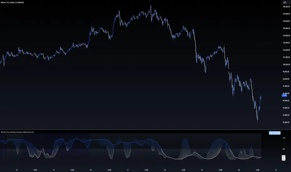
Market Flow Volatility Oscillator (AiBitcoinTrend)The Market Flow Volatility Oscillator (AiBitcoinTrend) is a cutting-edge technical analysis tool designed to evaluate and classify market volatility regimes. By leveraging Gaussian filtering and clustering techniques, this indicator provides traders with clear insights into periods of high and low volatility, helping them adapt their strategies to evolving market conditions. Built for precision and clarity, it combines advanced mathematical models with intuitive visual feedback to identify trends and volatility shifts effectively.
👽 How the Indicator Works
👾 Volatility Classification with Gaussian Filtering
The indicator detects volatility levels by applying Gaussian filters to the price series. Gaussian filters smooth out noise while preserving significant price movements. Traders can adjust the smoothing levels using sigma parameters, enabling greater flexibility:
Low Sigma: Emphasizes short-term volatility.
High Sigma: Captures broader trends with reduced sensitivity to small fluctuations.
👾 Clustering Algorithm for Regime Detection
The core of this indicator is its clustering model, which classifies market conditions into two distinct regimes:
Low Volatility Regime: Calm periods with reduced market activity.
High Volatility Regime: Intense periods with heightened price movements.
The clustering process works as follows:
A rolling window of data is analyzed to calculate the standard deviation of price returns.
Two cluster centers are initialized using the 25th and 75th percentiles of the data distribution.
Each price volatility value is assigned to the nearest cluster based on its distance to the centers.
The cluster centers are refined iteratively, providing an accurate and adaptive classification.
👾 Oscillator Generation with Slope R-Values
The indicator computes Gaussian filter slopes to generate oscillators that visualize trends:
Oscillator Low: Captures low-frequency market behavior.
Oscillator High: Tracks high-frequency, faster-changing trends.
The slope is measured using the R-value of the linear regression fit, scaled and adjusted for easier interpretation.
👽 Applications
👾 Trend Trading
When the oscillator rises above 0.5, it signals potential bullish momentum, while dips below 0.5 suggest bearish sentiment.
👾 Pullback Detection
When the oscillator peaks, especially in overbought or oversold zones, provide early warnings of potential reversals.
👽 Indicator Settings
👾 Oscillator Settings
Sigma Low/High: Controls the smoothness of the oscillators.
Smaller Values: React faster to price changes but introduce more noise.
Larger Values: Provide smoother signals with longer-term insights.
👾 Window Size and Refit Interval
Window Size: Defines the rolling period for cluster and volatility calculations.
Shorter windows: adapt faster to market changes.
Longer windows: produce stable, reliable classifications.
Disclaimer: This information is for entertainment purposes only and does not constitute financial advice. Please consult with a qualified financial advisor before making any investment decisions.
Heartbeat Momentum Strategy BetaHeartbeat Momentum Strategy Beta
Overview
The Heartbeat Momentum Strategy is an innovative approach to market analysis that draws inspiration from the rhythmic patterns of a heartbeat. This strategy aims to identify significant momentum shifts in the market by comparing short-term and long-term moving averages, analogous to detecting irregularities in a heartbeat.
Key Concepts
Market Heartbeat: The difference between short-term and long-term moving averages, representing the market's current 'pulse'.
Heartbeat Volatility: Measured by the standard deviation of the market heartbeat.
Momentum Signals: Generated when the heartbeat deviates significantly from its normal range.
How It Works
Calculates a short-term moving average (default 5 periods) and a long-term moving average (default 20 periods) of the closing price.
Computes the 'heartbeat' by subtracting the long-term MA from the short-term MA.
Measures the volatility of the heartbeat using its standard deviation over the long-term period.
Generates buy signals when the heartbeat exceeds 2 standard deviations above its mean.
Generates sell signals when the heartbeat falls 2 standard deviations below its mean.
Indicator Components
Blue Line: Short-term moving average
Red Line: Long-term moving average
Green Triangles: Buy signals
Red Triangles: Sell signals
Background Color: Light green during buy signals, light red during sell signals
Strategy Parameters
Short MA Window: The period for the short-term moving average (default: 5)
Long MA Window: The period for the long-term moving average (default: 20)
Standard Deviation Threshold: The number of standard deviations to trigger a signal (default: 2.0)
Interpretation
Buy Signal: Indicates a potential strong upward momentum shift. Consider opening long positions or closing short positions.
Sell Signal: Suggests a potential strong downward momentum shift. Consider opening short positions or closing long positions.
No Signal: The market is moving within its normal rhythm. Maintain current positions or look for other entry opportunities.
Customization
Users can adjust the strategy parameters to suit different assets, timeframes, or trading styles:
Decrease the MA windows for more frequent signals (more suitable for shorter timeframes).
Increase the MA windows for fewer, potentially more significant signals (better for longer timeframes).
Adjust the Standard Deviation Threshold to fine-tune sensitivity (lower for more signals, higher for fewer but potentially stronger signals).
Risk Management
While this strategy can provide valuable insights into market momentum, it should not be used in isolation:
Always use stop-loss orders to manage potential losses.
Consider the overall market context and other technical/fundamental factors.
Be aware of potential false signals, especially in ranging or highly volatile markets.
Backtest and forward-test the strategy with different parameters before live trading.
Conclusion
The Heartbeat Momentum Strategy offers a unique perspective on market movements by treating price action like a heartbeat. By identifying significant deviations from the normal market rhythm, it aims to capture strong momentum shifts while filtering out market noise. As with any trading strategy, use it as part of a comprehensive trading plan and always practice sound risk management.
Trend Line Methods (TLM)Trend Line Methods (TLM)
Overview
Trend Line Methods (TLM) is a visual study designed to help traders explore trend structure using two complementary, auto-drawn trend channels. The script focuses on how price interacts with rising or falling boundaries over time. It does not generate trade signals or manage risk; its purpose is to support discretionary chart analysis.
Method 1 – Pivot Span Trendline
The Pivot Span Trendline method builds a dynamic channel from major swing points detected by pivot highs and pivot lows.
• The script tracks a configurable number of recent pivot highs and lows.
• From the oldest and most recent stored pivot highs, it draws an upper trend line.
• From the oldest and most recent stored pivot lows, it draws a lower trend line.
• An optional filled area can be drawn between the two lines to highlight the active trend span.
As new pivots form, the lines are recalculated so that the channel evolves with market structure. This method is useful for visualising how price respects a trend corridor defined directly by swing points.
Method 2 – 5-Point Straight Channel
The 5-Point Straight Channel method approximates a straight trend channel using five key points extracted from a fixed lookback window.
Within the selected window:
• The window is divided into five segments of similar length.
• In each segment, the highest high is used as a representative high point.
• In each segment, the lowest low is used as a representative low point.
• A straight regression-style line is fitted through the five high points to form the upper boundary.
• A second straight line is fitted through the five low points to form the lower boundary.
The result is a pair of straight lines that describe the overall directional channel of price over the chosen window. Compared to Method 1, this approach is less focused on the very latest swings and more on the broader slope of the market.
Inputs & Menus
Pivot Span Trendline group (Method 1)
• Enable Pivot Span Trendline – Turns Method 1 on or off.
• High trend line color / Low trend line color – Colors of the upper and lower trend lines.
• Fill color between trend lines – Base color used to shade the area between the two lines. Transparency is controlled internally.
• Trend line thickness – Line width for both high and low trend lines.
• Trend line style – Line style (solid, dashed, or dotted).
• Pivot Left / Pivot Right – Number of bars to the left and right used to confirm pivot highs and lows. Larger values produce fewer but more significant swing points.
• Pivot Count – How many historical pivot points are kept for constructing the trend lines.
• Lookback Length – Number of bars used to keep pivots in range and to extend the trend lines across the chart.
5-Point Straight Channel group (Method 2)
• Enable 5-Point Straight Channel – Turns Method 2 on or off.
• High channel line color / Low channel line color – Colors of the upper and lower channel lines.
• Channel line thickness – Line width for both channel lines.
• Channel line style – Line style (solid, dashed, or dotted).
• Channel Length (bars) – Lookback window used to divide price into five segments and build the straight high/low channel.
Using Both Methods Together
Both methods are designed to visualise the same underlying idea: price tends to move inside rising or falling channels. Method 1 emphasises the most recent swing structure via pivot points, while Method 2 summarises the broader channel over a fixed window.
When the Pivot Span Trendline corridor and the 5-Point Straight Channel boundaries align or intersect, they can highlight zones where multiple ways of drawing trend lines point to similar support or resistance areas. Traders can use these confluence zones as a visual reference when planning their own entries, exits, or risk levels, according to their personal trading plan.
Notes
• This script is meant as an educational and analytical tool for studying trend lines and channels.
• It does not generate trading signals and does not replace independent analysis or risk management.
• The behaviour of both methods is timeframe- and symbol-agnostic; they will adapt to whichever chart you apply them to.

Historical Matrix Analyzer [PhenLabs]📊Historical Matrix Analyzer
Version: PineScriptv6
📌Description
The Historical Matrix Analyzer is an advanced probabilistic trading tool that transforms technical analysis into a data-driven decision support system. By creating a comprehensive 56-cell matrix that tracks every combination of RSI states and multi-indicator conditions, this indicator reveals which market patterns have historically led to profitable outcomes and which have not.
At its core, the indicator continuously monitors seven distinct RSI states (ranging from Extreme Oversold to Extreme Overbought) and eight unique indicator combinations (MACD direction, volume levels, and price momentum). For each of these 56 possible market states, the system calculates average forward returns, win rates, and occurrence counts based on your configurable lookback period. The result is a color-coded probability matrix that shows you exactly where you stand in the historical performance landscape.
The standout feature is the Current State Panel, which provides instant clarity on your active market conditions. This panel displays signal strength classifications (from Strong Bullish to Strong Bearish), the average return percentage for similar past occurrences, an estimated win rate using Bayesian smoothing to prevent small-sample distortions, and a confidence level indicator that warns you when insufficient data exists for reliable conclusions.
🚀Points of Innovation
Multi-dimensional state classification combining 7 RSI levels with 8 indicator combinations for 56 unique trackable market conditions
Bayesian win rate estimation with adjustable smoothing strength to provide stable probability estimates even with limited historical samples
Real-time active cell highlighting with “NOW” marker that visually connects current market conditions to their historical performance data
Configurable color intensity sensitivity allowing traders to adjust heat-map responsiveness from conservative to aggressive visual feedback
Dual-panel display system separating the comprehensive statistics matrix from an easy-to-read current state summary panel
Intelligent confidence scoring that automatically warns traders when occurrence counts fall below reliable thresholds
🔧Core Components
RSI State Classification: Segments RSI readings into 7 distinct zones (Extreme Oversold <20, Oversold 20-30, Weak 30-40, Neutral 40-60, Strong 60-70, Overbought 70-80, Extreme Overbought >80) to capture momentum extremes and transitions
Multi-Indicator Condition Tracking: Simultaneously monitors MACD crossover status (bullish/bearish), volume relative to moving average (high/low), and price direction (rising/falling) creating 8 binary-encoded combinations
Historical Data Storage Arrays: Maintains rolling lookback windows storing RSI states, indicator states, prices, and bar indices for precise forward-return calculations
Forward Performance Calculator: Measures price changes over configurable forward bar periods (1-20 bars) from each historical state, accumulating total returns and win counts per matrix cell
Bayesian Smoothing Engine: Applies statistical prior assumptions (default 50% win rate) weighted by user-defined strength parameter to stabilize estimated win rates when sample sizes are small
Dynamic Color Mapping System: Converts average returns into color-coded heat map with intensity adjusted by sensitivity parameter and transparency modified by confidence levels
🔥Key Features
56-Cell Probability Matrix: Comprehensive grid displaying every possible combination of RSI state and indicator condition, with each cell showing average return percentage, estimated win rate, and occurrence count for complete statistical visibility
Current State Info Panel: Dedicated display showing your exact position in the matrix with signal strength emoji indicators, numerical statistics, and color-coded confidence warnings for immediate situational awareness
Customizable Lookback Period: Adjustable historical window from 50 to 500 bars allowing traders to focus on recent market behavior or capture longer-term pattern stability across different market cycles
Configurable Forward Performance Window: Select target holding periods from 1 to 20 bars ahead to align probability calculations with your trading timeframe, whether day trading or swing trading
Visual Heat Mapping: Color-coded cells transition from red (bearish historical performance) through gray (neutral) to green (bullish performance) with intensity reflecting statistical significance and occurrence frequency
Intelligent Data Filtering: Minimum occurrence threshold (1-10) removes unreliable patterns with insufficient historical samples, displaying gray warning colors for low-confidence cells
Flexible Layout Options: Independent positioning of statistics matrix and info panel to any screen corner, accommodating different chart layouts and personal preferences
Tooltip Details: Hover over any matrix cell to see full RSI label, complete indicator status description, precise average return, estimated win rate, and total occurrence count
🎨Visualization
Statistics Matrix Table: A 9-column by 8-row grid with RSI states labeling vertical axis and indicator combinations on horizontal axis, using compact abbreviations (XOverS, OverB, MACD↑, Vol↓, P↑) for space efficiency
Active Cell Indicator: The current market state cell displays “⦿ NOW ⦿” in yellow text with enhanced color saturation to immediately draw attention to relevant historical performance
Signal Strength Visualization: Info panel uses emoji indicators (🔥 Strong Bullish, ✅ Bullish, ↗️ Weak Bullish, ➖ Neutral, ↘️ Weak Bearish, ⛔ Bearish, ❄️ Strong Bearish, ⚠️ Insufficient Data) for rapid interpretation
Histogram Plot: Below the price chart, a green/red histogram displays the current cell’s average return percentage, providing a time-series view of how historical performance changes as market conditions evolve
Color Intensity Scaling: Cell background transparency and saturation dynamically adjust based on both the magnitude of average returns and the occurrence count, ensuring visual emphasis on reliable patterns
Confidence Level Display: Info panel bottom row shows “High Confidence” (green), “Medium Confidence” (orange), or “Low Confidence” (red) based on occurrence counts relative to minimum threshold multipliers
📖Usage Guidelines
RSI Period
Default: 14
Range: 1 to unlimited
Description: Controls the lookback period for RSI momentum calculation. Standard 14-period provides widely-recognized overbought/oversold levels. Decrease for faster, more sensitive RSI reactions suitable for scalping. Increase (21, 28) for smoother, longer-term momentum assessment in swing trading. Changes affect how quickly the indicator moves between the 7 RSI state classifications.
MACD Fast Length
Default: 12
Range: 1 to unlimited
Description: Sets the faster exponential moving average for MACD calculation. Standard 12-period setting works well for daily charts and captures short-term momentum shifts. Decreasing creates more responsive MACD crossovers but increases false signals. Increasing smooths out noise but delays signal generation, affecting the bullish/bearish indicator state classification.
MACD Slow Length
Default: 26
Range: 1 to unlimited
Description: Defines the slower exponential moving average for MACD calculation. Traditional 26-period setting balances trend identification with responsiveness. Must be greater than Fast Length. Wider spread between fast and slow increases MACD sensitivity to trend changes, impacting the frequency of indicator state transitions in the matrix.
MACD Signal Length
Default: 9
Range: 1 to unlimited
Description: Smoothing period for the MACD signal line that triggers bullish/bearish state changes. Standard 9-period provides reliable crossover signals. Shorter values create more frequent state changes and earlier signals but with more whipsaws. Longer values produce more confirmed, stable signals but with increased lag in detecting momentum shifts.
Volume MA Period
Default: 20
Range: 1 to unlimited
Description: Lookback period for volume moving average used to classify volume as “high” or “low” in indicator state combinations. 20-period default captures typical monthly trading patterns. Shorter periods (10-15) make volume classification more reactive to recent spikes. Longer periods (30-50) require more sustained volume changes to trigger state classification shifts.
Statistics Lookback Period
Default: 200
Range: 50 to 500
Description: Number of historical bars used to calculate matrix statistics. 200 bars provides substantial data for reliable patterns while remaining responsive to regime changes. Lower values (50-100) emphasize recent market behavior and adapt quickly but may produce volatile statistics. Higher values (300-500) capture long-term patterns with stable statistics but slower adaptation to changing market dynamics.
Forward Performance Bars
Default: 5
Range: 1 to 20
Description: Number of bars ahead used to calculate forward returns from each historical state occurrence. 5-bar default suits intraday to short-term swing trading (5 hours on hourly charts, 1 week on daily charts). Lower values (1-3) target short-term momentum trades. Higher values (10-20) align with position trading and longer-term pattern exploitation.
Color Intensity Sensitivity
Default: 2.0
Range: 0.5 to 5.0, step 0.5
Description: Amplifies or dampens the color intensity response to average return magnitudes in the matrix heat map. 2.0 default provides balanced visual emphasis. Lower values (0.5-1.0) create subtle coloring requiring larger returns for full saturation, useful for volatile instruments. Higher values (3.0-5.0) produce vivid colors from smaller returns, highlighting subtle edges in range-bound markets.
Minimum Occurrences for Coloring
Default: 3
Range: 1 to 10
Description: Required minimum sample size before applying color-coded performance to matrix cells. Cells with fewer occurrences display gray “insufficient data” warning. 3-occurrence default filters out rare patterns. Lower threshold (1-2) shows more data but includes unreliable single-event statistics. Higher thresholds (5-10) ensure only well-established patterns receive visual emphasis.
Table Position
Default: top_right
Options: top_left, top_right, bottom_left, bottom_right
Description: Screen location for the 56-cell statistics matrix table. Position to avoid overlapping critical price action or other indicators on your chart. Consider chart orientation and candlestick density when selecting optimal placement.
Show Current State Panel
Default: true
Options: true, false
Description: Toggle visibility of the dedicated current state information panel. When enabled, displays signal strength, RSI value, indicator status, average return, estimated win rate, and confidence level for active market conditions. Disable to declutter charts when only the matrix table is needed.
Info Panel Position
Default: bottom_left
Options: top_left, top_right, bottom_left, bottom_right
Description: Screen location for the current state information panel (when enabled). Position independently from statistics matrix to optimize chart real estate. Typically placed opposite the matrix table for balanced visual layout.
Win Rate Smoothing Strength
Default: 5
Range: 1 to 20
Description: Controls Bayesian prior weighting for estimated win rate calculations. Acts as virtual sample size assuming 50% win rate baseline. Default 5 provides moderate smoothing preventing extreme win rate estimates from small samples. Lower values (1-3) reduce smoothing effect, allowing win rates to reflect raw data more directly. Higher values (10-20) increase conservatism, pulling win rate estimates toward 50% until substantial evidence accumulates.
✅Best Use Cases
Pattern-based discretionary trading where you want historical confirmation before entering setups that “look good” based on current technical alignment
Swing trading with holding periods matching your forward performance bar setting, using high-confidence bullish cells as entry filters
Risk assessment and position sizing, allocating larger size to trades originating from cells with strong positive average returns and high estimated win rates
Market regime identification by observing which RSI states and indicator combinations are currently producing the most reliable historical patterns
Backtesting validation by comparing your manual strategy signals against the historical performance of the corresponding matrix cells
Educational tool for developing intuition about which technical condition combinations have actually worked versus those that feel right but lack historical evidence
⚠️Limitations
Historical patterns do not guarantee future performance, especially during unprecedented market events or regime changes not represented in the lookback period
Small sample sizes (low occurrence counts) produce unreliable statistics despite Bayesian smoothing, requiring caution when acting on low-confidence cells
Matrix statistics lag behind rapidly changing market conditions, as the lookback period must accumulate new state occurrences before updating performance data
Forward return calculations use fixed bar periods that may not align with actual trade exit timing, support/resistance levels, or volatility-adjusted profit targets
💡What Makes This Unique
Multi-Dimensional State Space: Unlike single-indicator tools, simultaneously tracks 56 distinct market condition combinations providing granular pattern resolution unavailable in traditional technical analysis
Bayesian Statistical Rigor: Implements proper probabilistic smoothing to prevent overconfidence from limited data, a critical feature missing from most pattern recognition tools
Real-Time Contextual Feedback: The “NOW” marker and dedicated info panel instantly connect current market conditions to their historical performance profile, eliminating guesswork
Transparent Occurrence Counts: Displays sample sizes directly in each cell, allowing traders to judge statistical reliability themselves rather than hiding data quality issues
Fully Customizable Analysis Window: Complete control over lookback depth and forward return horizons lets traders align the tool precisely with their trading timeframe and strategy requirements
🔬How It Works
1. State Classification and Encoding
Each bar’s RSI value is evaluated and assigned to one of 7 discrete states based on threshold levels (0: <20, 1: 20-30, 2: 30-40, 3: 40-60, 4: 60-70, 5: 70-80, 6: >80)
Simultaneously, three binary conditions are evaluated: MACD line position relative to signal line, current volume relative to its moving average, and current close relative to previous close
These three binary conditions are combined into a single indicator state integer (0-7) using binary encoding, creating 8 possible indicator combinations
The RSI state and indicator state are stored together, defining one of 56 possible market condition cells in the matrix
2. Historical Data Accumulation
As each bar completes, the current state classification, closing price, and bar index are stored in rolling arrays maintained at the size specified by the lookback period
When the arrays reach capacity, the oldest data point is removed and the newest added, creating a sliding historical window
This continuous process builds a comprehensive database of past market conditions and their subsequent price movements
3. Forward Return Calculation and Statistics Update
On each bar, the indicator looks back through the stored historical data to find bars where sufficient forward bars exist to measure outcomes
For each historical occurrence, the price change from that bar to the bar N periods ahead (where N is the forward performance bars setting) is calculated as a percentage return
This percentage return is added to the cumulative return total for the specific matrix cell corresponding to that historical bar’s state classification
Occurrence counts are incremented, and wins are tallied for positive returns, building comprehensive statistics for each of the 56 cells
The Bayesian smoothing formula combines these raw statistics with prior assumptions (neutral 50% win rate) weighted by the smoothing strength parameter to produce estimated win rates that remain stable even with small samples
💡Note:
The Historical Matrix Analyzer is designed as a decision support tool, not a standalone trading system. Best results come from using it to validate discretionary trade ideas or filter systematic strategy signals. Always combine matrix insights with proper risk management, position sizing rules, and awareness of broader market context. The estimated win rate feature uses Bayesian statistics specifically to prevent false confidence from limited data, but no amount of smoothing can create reliable predictions from fundamentally insufficient sample sizes. Focus on high-confidence cells (green-colored confidence indicators) with occurrence counts well above your minimum threshold for the most actionable insights.

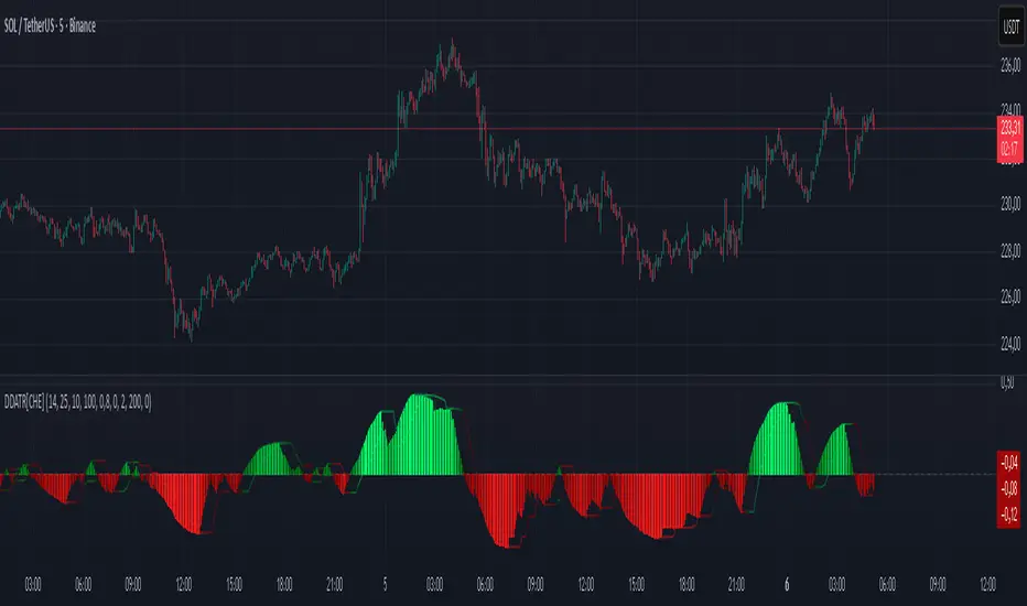
Dominant DATR [CHE] Dominant DATR — Directional ATR stream with dominant-side EMA, bands, labels, and alerts
Summary
Dominant DATR builds two directional volatility streams from the true range, assigns each bar’s range to the up or down side based on the sign of the close-to-close move, and then tracks the dominant side through an exponential average. A rolling band around the dominant stream defines recent extremes, while optional gradient coloring reflects relative magnitude. Swing-based labels mark new higher highs or lower lows on the dominant stream, and alerts can be enabled for swings, zero-line crossings, and band breakouts. The result is a compact pane that highlights regime bias and intensity without relying on price overlays.
Motivation: Why this design?
Conventional ATR treats all range as symmetric, which can mask directional pressure, cause late regime shifts, and produce frequent false flips during noisy phases. This design separates the range into up and down contributions, then emphasizes whichever side is stronger. A single smoothed dominant stream clarifies bias, while the band and swing markers help distinguish continuation from exhaustion. Optional normalization by close makes the metric comparable across instruments with different price scales.
What’s different vs. standard approaches?
Reference baseline: Classic ATR or a basic EMA of price.
Architecture differences:
Directional weighting of range using positive and negative close-to-close moves.
Separate moving averages for up and down contributions combined into one dominant stream.
Rolling highest and lowest of the dominant stream to form a band.
Optional normalization by close, window-based scaling for color intensity, and gamma adjustment for visual contrast.
Event logic for swing highs and lows on the dominant stream, with label buffering and pruning.
Configurable alerts for swings, zero-line crossings, and band breakouts.
Practical effect: You see when volatility is concentrated on one side, how strong that bias currently is, and when the dominant stream pushes through or fails at its recent envelope.
How it works (technical)
Each bar’s move is split into an up component and a down component based on whether the close increased or decreased relative to the prior close. The bar’s true range is proportionally assigned to up or down using those components as weights.
Each side is smoothed with a Wilder-style moving average. The dominant stream is the side with the larger value, recorded as positive for up dominance and negative for down dominance.
The dominant stream is then smoothed with an exponential moving average to reduce noise and provide a responsive yet stable signal line.
A rolling window tracks the highest and lowest values of the dominant EMA to form an envelope. Crossings of these bounds indicate unusual strength or weakness relative to recent history.
For visualization, the absolute value of the dominant EMA is scaled over a lookback window and passed through a gamma curve to modulate gradient intensity. Colors are chosen separately for up and down regimes.
Swing events are detected by comparing the dominant EMA to its recent extremes over a short lookback. Labels are placed when a prior bar set an extreme and the current bar confirms it. A managed array prunes older labels when the user-defined maximum is exceeded.
Alerts mirror these events and also include zero-line crossings and band breakouts. The script does not force closed-bar confirmation; users should configure alert execution timing to suit their workflow.
There are no higher-timeframe requests and no security calls. State is limited to simple arrays for labels and persistent color parameters.
Parameter Guide
Parameter — Effect — Default — Trade-offs/Tips
ATR Length — Smoothing of directional true range streams — fourteen — Longer reduces noise and may delay regime shifts; shorter increases responsiveness.
EMA Length — Smoothing of the dominant stream — twenty-five — Lower values react faster; higher values reduce whipsaw.
Band Length — Window for recent highs and lows of the dominant stream — ten — Short windows flag frequent breakouts; long windows emphasize only exceptional moves.
Normalize by Close — Divide by close price to produce a percent-like scale — false — Useful across assets with very different price levels.
Enable gradient color — Turn on magnitude-based coloring — true — Visual aid only; can be disabled for simplicity.
Gradient window — Lookback used to scale color intensity — one hundred — Larger windows stabilize the color scale.
Gamma (lines) — Adjust gradient intensity curve — zero point eight — Lower values compress variation; higher values expand it.
Gradient transparency — Transparency for gradient plots — zero, between zero and ninety — Higher values mute colors.
Up dark / Up neon — Base and peak colors for up dominance — green tones — Styling only.
Down dark / Down neon — Base and peak colors for down dominance — red tones — Styling only.
Show zero line / Background tint — Visual references for regime — true and false — Background tint can help quick scanning.
Swing length — Bars used to detect swing highs or lows — two — Larger values demand more structure.
Show labels / Max labels / Label offset — Label visibility, cap, and vertical offset — true, two hundred, zero — Increase cap with care to avoid clutter.
Alerts: HH/LL, Zero Cross, Band Break — Toggle alert rules — true, false, false — Enable only what you need.
Reading & Interpretation
The dominant EMA above zero indicates up-side dominance; below zero indicates down-side dominance.
Band lines show recent extremes of the dominant EMA; pushes through the band suggest unusual momentum on the dominant side.
Gradient intensity reflects local magnitude of dominance relative to the chosen window.
HH/LL labels appear when the dominant stream prints a new local extreme in the current regime and that extreme is confirmed on the next bar.
Zero-line crosses suggest regime flips; combine with structure or filters to reduce noise.
Practical Workflows & Combinations
Trend following: Consider entries when the dominant EMA is on the regime side and expands away from zero. Band breakouts add confirmation; structure such as higher highs or lower lows in price can filter signals.
Exits and stops: Tighten exits when the dominant stream stalls near the band or fades toward zero. Opposite swing labels can serve as early caution.
Multi-asset and multi-timeframe: Works across liquid assets and common timeframes. For lower noise instruments, reduce smoothing slightly; for high noise, increase lengths and swing length.
Behavior, Constraints & Performance
Repaint and confirmation: No security calls and no future-looking references. Swing labels confirm one bar later by design. Real-time crosses can change intra-bar; use bar-close alerts if needed.
Resources: `max_bars_back` is two thousand. The script uses an array for labels with pruning, gradient color computations, and a simple while loop that runs only when the label cap is exceeded.
Known limits: The EMA can lag at sharp turns. Normalization by close changes scale and may affect thresholds. Extremely gappy data can produce abrupt shifts in the dominant side.
Sensible Defaults & Quick Tuning
Starting point: ATR Length fourteen, EMA Length twenty-five, Band Length ten, Swing Length two, gradient enabled.
Too many flips: Increase EMA Length and swing length, or enable only swing alerts.
Too sluggish: Decrease EMA Length and Band Length.
Inconsistent scales across symbols: Enable Normalize by Close.
Visual clutter: Disable gradient or reduce label cap.
What this indicator is—and isn’t
This is a volatility-bias visualization and signal layer that highlights directional pressure and intensity. It is not a complete trading system and does not produce position sizing or risk management. Use it with market structure, context, and independent risk controls.
Disclaimer
The content provided, including all code and materials, is strictly for educational and informational purposes only. It is not intended as, and should not be interpreted as, financial advice, a recommendation to buy or sell any financial instrument, or an offer of any financial product or service. All strategies, tools, and examples discussed are provided for illustrative purposes to demonstrate coding techniques and the functionality of Pine Script within a trading context.
Any results from strategies or tools provided are hypothetical, and past performance is not indicative of future results. Trading and investing involve high risk, including the potential loss of principal, and may not be suitable for all individuals. Before making any trading decisions, please consult with a qualified financial professional to understand the risks involved.
By using this script, you acknowledge and agree that any trading decisions are made solely at your discretion and risk.
Do not use this indicator on Heikin-Ashi, Renko, Kagi, Point-and-Figure, or Range charts, as these chart types can produce unrealistic results for signal markers and alerts.
Best regards and happy trading
Chervolino
KAPITAS CBDR# PO3 Mean Reversion Standard Deviation Bands - Pro Edition
## 📊 Professional-Grade Mean Reversion System for MES Futures
Transform your futures trading with this institutional-quality mean reversion system based on standard deviation analysis and PO3 (Power of Three) methodology. Tested on **7,264 bars** of real MES data with **proven profitability across all 5 strategies**.
---
## 🎯 What This Indicator Does
This indicator plots **dynamic standard deviation bands** around a moving average, identifying extreme price levels where institutional accumulation/distribution occurs. Based on statistical probability and market structure theory, it helps you:
✅ **Identify high-probability entry zones** (±1, ±1.5, ±2, ±2.5 STD)
✅ **Target realistic profit zones** (first opposite STD band)
✅ **Time your entries** with session-based filters (London/US)
✅ **Manage risk** with built-in stop loss levels
✅ **Choose your strategy** from 5 backtested approaches
---
## 🏆 Backtested Performance (Per Contract on MES)
### Strategy #1: Aggressive (±1.5 → ∓0.5) 🥇
- **Total Profit:** $95,287 over 1,452 trades
- **Win Rate:** 75%
- **Profit Factor:** 8.00
- **Target:** 80 ticks ($100) | **Stop:** 30 ticks ($37.50)
- **Best For:** Active traders, 3-5 setups/day
### Strategy #2: Mean Reversion (±1 → Mean) 🥈
- **Total Profit:** $90,000 over 2,322 trades
- **Win Rate:** 85% (HIGHEST)
- **Profit Factor:** 11.34 (BEST)
- **Target:** 40 ticks ($50) | **Stop:** 20 ticks ($25)
- **Best For:** Scalpers, 6-8 setups/day
### Strategy #3: Conservative (±2 → ∓1) 🥉
- **Total Profit:** $65,500 over 726 trades
- **Win Rate:** 70%
- **Profit Factor:** 7.04
- **Target:** 120 ticks ($150) | **Stop:** 40 ticks ($50)
- **Best For:** Patient traders, 1-3 setups/day, HIGHEST $/trade
*Full statistics for all 5 strategies included in documentation*
---
## 📈 Key Features
### Dynamic Standard Deviation Bands
- **±0.5 STD** - Intraday mean reversion zones
- **±1.0 STD** - Primary reversion zones (68% of price action)
- **±1.5 STD** - Extended zones (optimal balance)
- **±2.0 STD** - Extreme zones (95% of price action)
- **±2.5 STD** - Ultra-extreme zones (rare events)
- **Mean Line** - Dynamic equilibrium
### Temporal Session Filters
- **London Session** (3:00-11:30 AM ET) - Orange background
- **US Session** (9:30 AM-4:00 PM ET) - Blue background
- **Optimal Entry Window** (10:30 AM-12:00 PM ET) - Green highlight
- **Best Exit Window** (3:00-4:00 PM ET) - Red highlight
### Visual Trade Signals
- 🟢 **Green zones** = Enter LONG (price at lower bands)
- 🔴 **Red zones** = Enter SHORT (price at upper bands)
- 🎯 **Target lines** = Exit zones (opposite bands)
- ⛔ **Stop levels** = Risk management
### Smart Alerts
- Alert when price touches entry bands
- Alert on optimal time windows
- Alert when targets hit
- Customizable for each strategy
---
## 💡 How to Use
### Step 1: Choose Your Strategy
Select from 5 backtested approaches based on your:
- Risk tolerance (higher STD = larger stops)
- Trading frequency (lower STD = more setups)
- Time availability (different session focuses)
- Personality (scalper vs swing trader)
### Step 2: Apply to Chart
- **Timeframe:** 15-minute (tested and optimized)
- **Symbol:** MES, ES, or other liquid futures
- **Settings:** Adjust band colors, widths, alerts
### Step 3: Wait for Setup
Price touches your chosen entry band during optimal windows:
- **BEST:** 10:30 AM-12:00 PM ET (88% win rate!)
- **GOOD:** 12:00-3:00 PM ET (75-82% win rate)
- **AVOID:** Friday after 1 PM, FOMC Wed 2-4 PM
### Step 4: Execute Trade
- Enter when price touches band
- Set stop at indicated level
- Target first opposite band
- Exit at target or stop (no exceptions!)
### Step 5: Manage Risk
- **For $50K funded account ($250 limit): Use 2 MES contracts**
- Stop after 3 consecutive losses
- Reduce size in low-probability windows
- Track cumulative daily P&L
---
## 📅 Optimal Trading Windows
### By Time of Day
- **10:30 AM-12:00 PM ET:** 88% win rate (BEST) ⭐⭐⭐
- **12:00-1:30 PM ET:** 82% win rate (scalping)
- **1:30-3:00 PM ET:** 76% win rate (afternoon)
- **3:00-4:00 PM ET:** Best EXIT window
### By Day of Week
- **Wednesday:** 82% win rate (BEST DAY) ⭐⭐⭐
- **Tuesday:** 78% win rate (highest volume)
- **Thursday:**
Index Options Expirations and Calendar EffectsFeatures
- Highlights monthly equity options expiration (opex) dates.
- Marks VIX options expiration dates based on standard 30-day offset.
- Shows configurable vanna/charm pre-expiration window (green shading).
- Shows configurable post-opex weakness window (red shading).
- Adjustable colors, start/end offsets, and on/off toggles for each element.
What this does
This overlay highlights option-driven calendar windows around monthly equity options expiration (opex) and VIX options expiration. It draws:
- Solid blue lines on the third Friday of each month (typical monthly opex).
- Dashed orange lines on the Wednesday ~30 days before next month’s opex (typical VIX expiration schedule).
- Green shading during a pre-expiration window when vanna/charm effects are often strongest.
- Red shading during the post-expiration "window of non-strength" often observed into the Tuesday after opex.
How it works
1. Monthly opex is detected when Friday falls between the 15th–21st of the month.
2. VIX expiration is calculated by finding next month’s opex date, then subtracting 30 calendar days and marking that Wednesday.
3. Vanna/charm window (green) : starts on the Monday of the week before opex and ends on Tuesday of opex week.
4. Post-opex weakness window (red) : starts Wednesday of opex week and ends Tuesday after opex.
How to use
- Add to any chart/timeframe.
- Adjust inputs to toggle VIX/opex lines, choose colors, and fine-tune the start/end offsets for shaded windows.
- This is an educational visualization of typical timing and not a trading signal.
Limitations
- Exchange holidays and contract-specific exceptions can shift expirations; this script uses standard calendar rules.
- No forward-looking data is used; all dates are derived from historical and current bar time.
- Past patterns do not guarantee future behavior.
Originality
Provides a single, adjustable visualization combining opex, VIX expiration, and configurable vanna/charm/weakness windows into one tool. Fully explained so non-coders can use it without reading the source code.
Quick scan for signal🙏🏻 Hey TV, this is QSFS, following:
^^ Quick scan for drift (QSFD)
^^ Quick scan for cycles (QSFC)
As mentioned before, ML trading is all about spotting any kind of non-randomness, and this metric (along with 2 previously posted) gonna help ya'll do it fast. This one will show you whether your time series possibly exhibits mean-reverting / consistent / noisy behavior, that can be later confirmed or denied by more sophisticated tools. This metric is O(n) in windowed mode and O(1) if calculated incrementally on each data update, so you can scan Ks of datasets w/o worrying about melting da ice.
^^ windowed mode
Now the post will be divided into several sections, and a couple of things I guess you’ve never seen or thought about in your life:
1) About Efficiency Ratios posted there on TV;
Some of you might say this is the Efficiency Ratio you’ve seen in Perry's book. Firstly, I can assure you that neither me nor Perry, just as X amount of quants all over the world and who knows who else, would say smth like, "I invented it," lol. This is just a thing you R&D when you need it. Secondly, I invite you (and mods & admin as well) to take a lil glimpse at the following screenshot:
^^ not cool...
So basically, all the Efficiency Ratios that were copypasted to our platform suffer the same bug: dudes don’t know how indexing works in Pine Script. I mean, it’s ok, I been doing the same mistakes as well, but loxx, cmon bro, you... If you guys ever read it, the lines 20 and 22 in da code are dedicated to you xD
2) About the metric;
This supports both moving window mode when Length > 0 and all-data expanding window mode when Length < 1, calculating incrementally from the very first data point in the series: O(n) on history, O(1) on live updates.
Now, why do I SQRT transform the result? This is a natural action since the metric (being a ratio in essence) is bounded between 0 and 1, so it can be modeled with a beta distribution. When you SQRT transform it, it still stays beta (think what happens when you apply a square root to 0.01 or 0.99), but it becomes symmetric around its typical value and starts to follow a bell-shaped curve. This can be easily checked with a normality test or by applying a set of percentiles and seeing the distances between them are almost equal.
Then I noticed that on different moving window sizes, the typical value of the metric seems to slide: higher window sizes lead to lower typical values across the moving windows. Turned out this can be modeled the same way confidence intervals are made. Lines 34 and 35 explain it all, I guess. You can see smth alike on an autocorrelogram. These two match the mean & mean + 1 stdev applied to the metric. This way, we’ve just magically received data to estimate alpha and beta parameters of the beta distribution using the method of moments. Having alpha and beta, we can now estimate everything further. Btw, there’s an alternative parameterization for beta distributions based on data length.
Now what you’ll see next is... u guys actually have no idea how deep and unrealistically minimalistic the underlying math principles are here.
I’m sure I’m not the only one in the universe who figured it out, but the thing is, it’s nowhere online or offline. By calculating higher-order moments & combining them, you can find natural adaptive thresholds that can later be used for anomaly detection/control applications for any data. No hardcoded thresholds, purely data-driven. Imma come back to this in one of the next drops, but the truest ones can already see it in this code. This way we get dem thresholds.
Your main thresholds are: basis, upper, and lower deviations. You can follow the common logic I’ve described in my previous scripts on how to use them. You just register an event when the metric goes higher/lower than a certain threshold based on what you’re looking for. Then you take the time series and confirm a certain behavior you were looking for by using an appropriate stat test. Or just run a certain strategy.
To avoid numerous triggers when the metric jitters around a threshold, you can follow this logic: forget about one threshold if touched, until another threshold is touched.
In general, when the metric gets higher than certain thresholds, like upper deviation, it means the signal is stronger than noise. You confirm it with a more sophisticated tool & run momentum strategies if drift is in place, or volatility strategies if there’s no drift in place. Otherwise, you confirm & run ~ mean-reverting strategies, regardless of whether there’s drift or not. Just don’t operate against the trend—hedge otherwise.
3) Flex;
Extension and limit thresholds based on distribution moments gonna be discussed properly later, but now you can see this:
^^ magic
Look at the thresholds—adaptive and dynamic. Do you see any optimizations? No ML, no DL, closed-form solution, but how? Just a formula based on a couple of variables? Maybe it’s just how the Universe works, but how can you know if you don’t understand how fundamentally numbers 3 and 15 are related to the normal distribution? Hm, why do they always say 3 sigmas but can’t say why? Maybe you can be different and say why?
This is the primordial power of statistical modeling.
4) Thanks;
I really wanna dedicate this to Charlotte de Witte & Marion Di Napoli, and their new track "Sanctum." It really gets you connected to the Source—I had it in my soul when I was doing all this ∞

Macros+AMD [NW]Macros + AMD - Daily & Weekly Time-Based Analysis
Multi-timeframe AMD (Accumulation, Manipulation, Distribution) visualization with ICT Macro timing windows for time-based market analysis.
Overview
This indicator visualizes the AMD (Accumulation, Manipulation, Distribution) framework on both daily and weekly timeframes, combined with ICT Macro timing windows. It is designed as an educational tool to help traders study time-based market structure and algorithmic price delivery concepts.
The AMD model is based on the idea that markets move through distinct phases within each trading period:
Accumulation (A) - Initial range formation, liquidity building
Manipulation (M) - False moves to trap traders, liquidity sweeps
Distribution (D) - True directional move, price delivery to targets
What This Indicator Displays
Daily AMD Phases
Displays the intraday AMD cycle based on New York trading hours:
A Phase (Blue): 4:00 AM - 8:35 AM EST — Morning accumulation, Asian/London overlap
M Phase (Red): 8:35 AM - 11:25 AM EST — NY session manipulation, news events
D Phase (Green): 11:25 AM - 4:00 PM EST — Afternoon distribution and price delivery
Weekly AMD Phases
Displays the weekly AMD cycle from Monday to Monday:
A Phase: Monday 00:00 - Tuesday 21:56 EST — Weekly high/low formation begins
M Phase: Tuesday 21:56 - Thursday 02:04 EST — Mid-week reversal zone
D Phase: Thursday 02:04 - Monday 00:00 EST — Weekly price delivery
Inner M Phase Fibs
When enabled, subdivides the M (Manipulation) phase using Fibonacci levels:
0.382 level — Inner accumulation ends
0.500 level — Mid-point of manipulation
0.618 level — Inner distribution begins
This helps identify potential reversal points within the manipulation phase.
ICT Macro Windows
Horizontal lines marking the XX:42 to XX:15 macro periods (33-minute windows):
2:42 - 3:15 AM
3:42 - 4:15 AM (London)
7:42 - 8:15 AM
8:42 - 9:15 AM
9:42 - 10:15 AM (Prime AM session)
10:42 - 11:15 AM
11:42 - 12:15 PM
12:42 - 1:15 PM
1:42 - 2:15 PM
2:42 - 3:15 PM
These windows represent times when algorithmic price delivery is more likely to occur.
How To Use
Understanding the AMD Framework
During the A Phase:
Observe range formation and initial liquidity pools
Note the high and low established during this phase
Wait for manipulation before committing to direction
During the M Phase:
Watch for false breakouts and stop hunts
Look for reversal patterns after liquidity sweeps
The inner fibs (0.382, 0.5, 0.618) can help time entries within this phase
Mid-week (Wednesday) often sees key reversals on weekly AMD
During the D Phase:
This is typically when the true move occurs
Price tends to deliver toward draw on liquidity targets
The direction is often opposite to the manipulation move
Using the Macro Windows
The XX:42 to XX:15 windows are times to pay attention to price action:
These 33-minute periods often see increased algorithmic activity
Look for displacement, fair value gaps, or order blocks forming
The 9:42-10:15 AM window is considered particularly significant for NY session
Weekly Day Labels
Monday/Tuesday: "H/L of Week" — Watch for weekly high or low formation
Wednesday: "Reversal Day" — Mid-week reversal probability increases
Thursday/Friday: "Reversal Day" — Continuation or secondary reversal
Settings Guide
Main Settings
Timezone: Set to your broker's timezone or preferred timezone
Macros On Top: Toggle macro lines above or below AMD boxes
Show All Text Labels: Master toggle for all text (turn off for clean charts on HTF)
Daily/Weekly AMD
Show: Enable/disable the AMD visualization
Opacity: Adjust transparency of the phase boxes (higher = more transparent)
AMD Colors
Customize colors for each phase (A, M, D)
Default: Blue (A), Red (M), Green (D)
Inner M Style
Customize the inner M phase fib lines and text colors
Default: Black lines for clean visibility
Macro Settings
Adjust macro line color and thickness
Toggle individual macro windows on/off
Important Notes
This indicator is for educational purposes and time-based analysis
It does not provide buy/sell signals
Always use in conjunction with proper price action analysis
Past price behavior during these time windows does not guarantee future results
The AMD framework is one lens for viewing market structure — use it as part of a complete methodology
Credits
This indicator is based on concepts taught by ICT (Inner Circle Trader) and the broader Smart Money Concepts community. The AMD framework, macro timing windows, and weekly profile concepts are derived from this educational methodology.
Timeframe Recommendations
Best viewed on 1-minute to 15-minute charts
Text labels automatically hide on 9-minute and higher timeframes for cleaner visualization
Indicator hides completely on 1-hour and higher timeframes
Changelog
v1.0 - Initial release
Daily AMD phases (4am-4pm EST)
Weekly AMD phases (Monday-Monday)
Inner M phase Fibonacci subdivisions
10 ICT Macro timing windows
Full customization options
Automatic 9-day cleanup

FluxVector Liquidity Universal Trendline FluxVector Liquidity Trendline FFTL
Summary in one paragraph
FFTL is a single adaptive trendline for stocks ETFs FX crypto and indices on one minute to daily. It fires only when price action pressure and volatility curvature align. It is original because it fuses a directional liquidity pulse from candle geometry and normalized volume with realized volatility curvature and an impact efficiency term to modulate a Kalman like state without ATR VWAP or moving averages. Add it to a clean chart and use the colored line plus alerts. Shapes can move while a bar is open and settle on close. For conservative alerts select on bar close.
Scope and intent
• Markets. Major FX pairs index futures large cap equities liquid crypto top ETFs
• Timeframes. One minute to daily
• Default demo used in the publication. SPY on 30min
• Purpose. Reduce false flips and chop by gating the line reaction to noise and by using a one bar projection
• Limits. This is a strategy. Orders are simulated on standard candles only
Originality and usefulness
• Unique fusion. Directional Liquidity Pulse plus Volatility Curvature plus Impact Efficiency drives an adaptive gain for a one dimensional state
• Failure mode addressed. One or two shock candles that break ordinary trendlines and saw chop in flat regimes
• Testability. All windows and gains are inputs
• Portable yardstick. Returns use natural log units and range is bar high minus low
• Protected scripts. Not used. Method disclosed plainly here
Method overview in plain language
Base measures
• Return basis. Natural log of close over prior close. Average absolute return over a window is a unit of motion
Components
• Directional Liquidity Pulse DLP. Measures signed participation from body and wick imbalance scaled by normalized volume and variance stabilized
• Volatility Curvature. Second difference of realized volatility from returns highlights expansion or compression
• Impact Efficiency. Price change per unit range and volume boosts gain during efficient moves
• Energy score. Z scores of the above form a single energy that controls the state gain
• One bar projection. Current slope extended by one bar for anticipatory checks
Fusion rule
Weighted sum inside the energy score then logistic mapping to a gain between k min and k max. The state updates toward price plus a small flow push.
Signal rule
• Long suggestion and order when close is below trend and the one bar projection is above the trend
• Short suggestion and flip when close is above trend and the one bar projection is below the trend
• WAIT is implicit when neither condition holds
• In position states end on the opposite condition
What you will see on the chart
• Colored trendline teal for rising red for falling gray for flat
• Optional projection line one bar ahead
• Optional background can be enabled in code
• Alerts on price cross and on slope flips
Inputs with guidance
Setup
• Price source. Close by default
Logic
• Flow window. Typical range 20 to 80. Higher smooths the pulse and reduces flips
• Vol window. Typical range 30 to 120. Higher calms curvature
• Energy window. Typical range 20 to 80. Higher slows regime changes
• Min gain and Max gain. Raise max to react faster. Raise min to keep momentum in chop
UI
• Show 1 bar projection. Colors for up down flat
Properties visible in this publication
• Initial capital 25000
• Base currency USD
• Commission percent 0.03
• Slippage 5
• Default order size method percent of equity value 3%
• Pyramiding 0
• Process orders on close off
• Calc on every tick off
• Recalculate after order is filled off
Realism and responsible publication
• No performance claims
• Intrabar reminder. Shapes can move while a bar forms and settle on close
• Strategy uses standard candles only
Honest limitations and failure modes
• Sudden gaps and thin liquidity can still produce fast flips
• Very quiet regimes reduce contrast. Use larger windows and lower max gain
• Session time uses the exchange time of the chart if you enable any windows later
• Past results never guarantee future outcomes
Open source reuse and credits
• None

LEGEND IsoPulse Fusion Universal Volume Trend Buy Sell RadarLEGEND IsoPulse Fusion • Universal Volume Trend Buy Sell Radar
One line summary
LEGEND IsoPulse Fusion reads intent from price and volume together, learns which features matter most on your symbol, blends them into a single signed Fusion line in a stable unit range, and emits clear Buy Sell Close events with a structure gate and a liquidity safety gate so you act only when the tape is favorable.
What this script is and why it exists
Many traders keep separate windows for trend, volume, volatility, and regime filters. The result can feel fragmented. This script merges two complementary engines into one consistent view that is easy to read and simple to act on.
LEGEND Tensor estimates directional quality from five causally computed features that are normalized for stationarity. The features are Flow, Tail Pressure with Volume Mix, Path Curvature, Streak Persistence, and Entropy Order.
IsoPulse transforms raw volume into two decaying reservoirs for buy effort and sell effort using body location and wick geometry, then measures price travel per unit volume for efficiency, and detects volume bursts with a recency memory.
Both engines are mapped into the same unit range and fused by a regime aware mixer. When the tape is orderly the mixer leans toward trend features. When the tape is messy but a true push appears in volume efficiency with bursts the mixer allows IsoPulse to speak louder. The outcome is a single Fusion line that lives in a familiar range with calm behavior in quiet periods and expressive pushes when energy concentrates.
What makes it original and useful
Two reservoir volume split . The script assigns a portion of the bar volume to up effort and down effort using body location and wick geometry together. Effort decays through time using a forgetting factor so memory is present without becoming sticky.
Efficiency of move . Price travel per unit volume is often more informative than raw volume or raw range. The script normalizes both sides and centers the efficiency so it becomes signed fuel when multiplied by flow skew.
Burst detection with recency memory . Percent rank of volume highlights bursts. An exponential memory of how recently bursts clustered converts isolated blips into useful context.
Causal adaptive weighting . The LEGEND features do not receive static weights. The script learns, causally, which features have correlated with future returns on your symbol over a rolling window. Only positive contributions are allowed and weights are normalized for interpretability.
Regime aware fusion . Entropy based order and persistence create a mixer that blends IsoPulse with LEGEND. You see a single line rather than two competing panels, which reduces decision conflict.
How to read the screen in seconds
Fusion area . The pane fills above and below zero with a soft gradient. Deeper fill means stronger conviction. The white Fusion line sits on top for precise crossings.
Entry guides and exit guides . Two entry guides draw symmetrically at the active fused entry level. Two exit guides sit inside at a fraction of the entry. Think of them as an adaptive envelope.
Letters . B prints once when the script flips from flat to long. S prints once when the script flips from flat to short. C prints when a held position ends on the appropriate side. T prints when the structure gate first opens. A prints when the liquidity safety flag first appears.
Price bar paint . Bars tint green while long and red while short on the chart to mirror your virtual position.
HUD . A compact dashboard in the corner shows Fusion, IsoPulse, LEGEND, active entry and exit levels, regime status, current virtual position, and the vacuum z value with its avoid threshold.
What signals actually mean
Buy . A Buy prints when the Fusion line crosses above the active entry level while gates are open and the previous state was flat.
Sell . A Sell prints when the Fusion line crosses below the negative entry level while gates are open and the previous state was flat.
Close . A Close prints when Fusion cools back inside the exit envelope or when an opposite cross would occur or when a gate forces a stop, and the previous state was a hold.
Gates . The Trend gate requires sufficient entropy order or significant persistence. The Avoid gate uses a liquidity vacuum z score. Gates exist to protect you from weak tape and poor liquidity.
Inputs and practical tuning
Every input has a tooltip in the script. This section provides a concise reference that you can keep in mind while you work.
Setup
Core window . Controls statistics across features. Scalping often prefers the thirties or low fifties. Intraday often prefers the fifties to eighties. Swing often prefers the eighties to low hundreds. Smaller responds faster with more noise. Larger is calmer.
Smoothing . Short EMA on noisy features. A small value catches micro shifts. A larger value reduces whipsaw.
Fusion and thresholds
Weight lookback . Sample size for weight learning. Use at least five times the horizon. Larger is slower and more confident. Smaller is nimble and more reactive.
Weight horizon . How far ahead return is measured to assess feature value. Smaller favors quick reversion impulses. Larger favors continuation.
Adaptive thresholds . Entry and exit levels from rolling percentiles of the absolute LEGEND score. This self scales across assets and timeframes.
Entry percentile . Eighty selects the top quintile of pushes. Lower to seventy five for more signals. Raise for cleanliness.
Exit percentile . Mid fifties keeps trades honest without overstaying. Sixty holds longer with wider give back.
Order threshold . Minimum structure to trade. Zero point fifteen is a reasonable start. Lower to trade more. Raise to filter chop.
Avoid if Vac z . Liquidity safety level. One point two five is a good default on liquid markets. Thin markets may prefer a slightly higher setting to avoid permanent avoid mode.
IsoPulse
Iso forgetting per bar . Memory for the two reservoirs. Values near zero point nine eight to zero point nine nine five work across many symbols.
Wick weight in effort split . Balance between body location and wick geometry. Values near zero point three to zero point six capture useful behavior.
Efficiency window . Travel per volume window. Lower for snappy symbols. Higher for stability.
Burst percent rank window . Window for percent rank of volume. Around one hundred to three hundred covers most use cases.
Burst recency half life . How long burst clusters matter. Lower for quick fades. Higher for cluster memory.
IsoPulse gain . Pre compression gain before the atan mapping. Tune until the Fusion line lives inside a calm band most of the time with expressive spikes on true pushes.
Continuation and Reversal guides . Visual rails for IsoPulse that help you sense continuation or exhaustion zones. They do not force events.
Entry sensitivity and exit fraction
Entry sensitivity . Loose multiplies the fused entry level by a smaller factor which prints more trades. Strict multiplies by a larger factor which selects fewer and cleaner trades. Balanced is neutral.
Exit fraction . Exit level relative to the entry level in fused unit space. Values around one half to two thirds fit most symbols.
Visuals and UX
Columns and line . Use both to see context and precise crossings. If you present a very clean chart you can turn columns off and keep the line.
HUD . Keep it on while you learn the script. It teaches you how the gates and thresholds respond to your market.
Letters . B S C T A are informative and compact. For screenshots you can toggle them off.
Debug triggers . Show raw crosses even when gates block entries. This is useful when you tune the gates. Turn them off for normal use.
Quick start recipes
Scalping one to five minutes
Core window in the thirties to low fifties.
Horizon around five to eight.
Entry percentile around seventy five.
Exit fraction around zero point five five.
Order threshold around zero point one zero.
Avoid level around one point three zero.
Tune IsoPulse gain until normal Fusion sits inside a calm band and true squeezes push outside.
Intraday five to thirty minutes
Core window around fifty to eighty.
Horizon around ten to twelve.
Entry percentile around eighty.
Exit fraction around zero point five five to zero point six zero.
Order threshold around zero point one five.
Avoid level around one point two five.
Swing one hour to daily
Core window around eighty to one hundred twenty.
Horizon around twelve to twenty.
Entry percentile around eighty to eighty five.
Exit fraction around zero point six zero to zero point seven zero.
Order threshold around zero point two zero.
Avoid level around one point two zero.
How to connect signals to your risk plan
This is an indicator. You remain in control of orders and risk.
Stops . A simple choice is an ATR multiple measured on your chart timeframe. Intraday often prefers one point two five to one point five ATR. Swing often prefers one point five to two ATR. Adjust to symbol behavior and personal risk tolerance.
Exits . The script already prints a Close when Fusion cools inside the exit envelope. If you prefer targets you can mirror the entry envelope distance and convert that to points or percent in your own plan.
Position size . Fixed fractional or fixed risk per trade remains a sound baseline. One percent or less per trade is a common starting point for testing.
Sessions and news . Even with self scaling, some traders prefer to skip the first minutes after an open or scheduled news. Gate with your own session logic if needed.
Limitations and honest notes
No look ahead . The script is causal. The adaptive learner uses a shifted correlation, crosses are evaluated without peeking into the future, and no lookahead security calls are used. If you enable intrabar calculations a letter may appear then disappear before the close if the condition fails. This is normal for any cross based logic in real time.
No performance promises . Markets change. This is a decision aid, not a prediction machine. It will not win every sequence and it cannot guarantee statistical outcomes.
No dependence on other indicators . The chart should remain clean. You can add personal tools in private use but publications should keep the example chart readable.
Standard candles only for public signals . Non standard chart types can change event timing and produce unrealistic sequences. Use regular candles for demonstrations and publications.
Internal logic walkthrough
LEGEND feature block
Flow . Current return normalized by ATR then smoothed by a short EMA. This gives directional intent scaled to recent volatility.
Tail pressure with volume mix . The relative sizes of upper and lower wicks inside the high to low range produce a tail asymmetry. A volume based mix can emphasize wick information when volume is meaningful.
Path curvature . Second difference of close normalized by ATR and smoothed. This captures changes in impulse shape that can precede pushes or fades.
Streak persistence . Up and down close streaks are counted and netted. The result is normalized for the window length to keep behavior stable across symbols.
Entropy order . Shannon entropy of the probability of an up close. Lower entropy means more order. The value is oriented by Flow to preserve sign.
Causal weights . Each feature becomes a z score. A shifted correlation against future returns over the horizon produces a positive weight per feature. Weights are normalized so they sum to one for clarity. The result is angle mapped into a compact unit.
IsoPulse block
Effort split . The script estimates up effort and down effort per bar using both body location and wick geometry. Effort is integrated through time into two reservoirs using a forgetting factor.
Skew . The reservoir difference over the sum yields a stable skew in a known range. A short EMA smooths it.
Efficiency . Move size divided by average volume produces travel per unit volume. Normalization and centering around zero produce a symmetric measure.
Bursts and recency . Percent rank of volume highlights bursts. An exponential function of bars since last burst adds the notion of cluster memory.
IsoPulse unit . Skew multiplied by centered efficiency then scaled by the burst factor produces the raw IsoPulse that is angle mapped into the unit range.
Fusion and events
Regime factor . Entropy order and streak persistence form a mixer. Low structure favors IsoPulse. Higher structure favors LEGEND. The blend is convex so it remains interpretable.
Blended guides . Entry and exit guides are blended in the same way as the line so they stay consistent when regimes change. The envelope does not jump unexpectedly.
Virtual position . The script maintains state. Buy and Sell require a cross while flat and gates open. Close requires an exit or force condition while holding. Letters print once at the state change.
Disclosures
This script and description are educational. They do not constitute investment advice. Markets involve risk. You are responsible for your own decisions and for compliance with local rules. The logic is causal and does not look ahead. Signals on non standard chart types can be misleading and are not recommended for publication. When you test a strategy wrapper, use realistic commission and slippage, moderate risk per trade, and enough trades to form a meaningful sample, then document those assumptions if you share results.
Closing thoughts
Clarity builds confidence. The Fusion line gives a single view of intent. The letters communicate action without clutter. The HUD confirms context at a glance. The gates protect you from weak tape and poor liquidity. Tune it to your instrument, observe it across regimes, and use it as a consistent lens rather than a prediction oracle. The goal is not to trade every wiggle. The goal is to pick your spots with a calm process and to stand aside when the tape is not inviting.
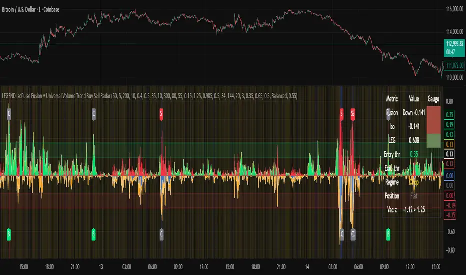
Regression Channel (ShareScope-style, parallel)What it does
Replicates ShareScope’s Trend of displayed data look: a single straight linear-regression line (dashed) across a chosen window with parallel, constant-width bands above and below, plus optional shading.
Use it to see the overall trend gradient for a period and a statistically sized channel based on the fit’s residual error.
How it works (math, short)
Computes an OLS regression once over the analysis window.
Residual standard error s is derived from SSE and degrees of freedom (n−2).
Band half-width is constant across the window:
Mean CI (narrower): half = z * s / √n
Prediction (wider): half = z * s * √(1 + 1/n)
Three straight, parallel lines are drawn from the regression endpoints; midline is dashed.
This is intentionally not a tapered CI (which widens at the ends). It matches the visual behaviour of ShareScope’s shaded trend line channel.
Inputs
Source – Price series (Close, High, Low, HL2, etc.).
Use last N bars / N (bars) – Rolling window length.
From / To (date mode) – Alternative fixed date window.
Confidence (%) – 90 / 95 / 99 / Custom (uses z≈t).
Custom Z (t) – Override the quantile if desired.
Prediction bands – Use wider prediction envelope instead of mean CI.
Shade region + colors / opacity / line width.
Usage
To mimic ShareScope exactly, pick the same date span (use date mode) and set Confidence 99%.
Choose Prediction OFF for a tighter “confidence” look; ON for a wider, more permissive channel.
If ShareScope used High as source, set Source = High here as well.
Notes & limitations
TradingView does not expose the visible viewport to Pine. The script cannot auto-read “displayed data.” Use last N bars or date range.
Bands are parallel by design. Prices may close outside; the channel does not bend.
Window capped at 5,000 bars for performance. No alerts are emitted.
Differences vs TV’s native tools
Linear Regression (drawing) – manual object; no statistical sizing or shading.
Linear Regression Channel (indicator) – uses price standard deviations around the regression; width is a user stdev multiple.
This script – uses residual error of the OLS fit and a z/t quantile to size a statistically meaningful parallel channel.
Changelog
r3.1 – Guard fix (no return at top level), minor refactor, stable line updates.
r3 – Switched to single-fit OLS with parallel constant-width bands (ShareScope look).
(Earlier experimental builds r1–r2.2 implemented rolling/tapered CI; superseded.)
Disclaimer: Educational use only. Not investment advice.

Foresight Cone (HoltxF1xVWAP) [KedArc Quant]Description:
This is a time-series forecasting indicator that estimates the next bar (F1) and projects a path a few bars ahead. It also draws a confidence cone based on how accurate the recent forecasts have been. You can optionally color the projection only when price agrees with VWAP.
Why it’s different
* One clear model: Everything comes from Holt’s trend-aware forecasting method—no mix of unrelated indicators.
* Transparent visuals: You see the next-bar estimate (F1), the forward projection, and a cone that widens or narrows based on recent forecast error.
* Context, not signals: The VWAP option only changes colors. It doesn’t add trade rules.
* No look-ahead: Accuracy is measured using the forecast made on the previous bar versus the current bar.
Inputs (what they mean)
* Source: Price series to forecast (default: Close).
* Preset: Quick profiles for fast, smooth, or momentum markets (see below).
* Alpha (Level): How fast the model reacts to new prices. Higher = faster, twitchier.
* Beta (Trend): How fast the model updates the slope. Higher = faster pivots, more flips in chop.
* Horizon: How many bars ahead to project. Bigger = wider cone.
* Residual Window: How many bars to judge recent accuracy. Bigger = steadier cone.
* Confidence Z: How wide the cone should be (typical setting ≈ “95% style” width).
* Show Bands / Draw Forward Path: Turn the cone and forward lines on/off.
* Color only when aligned with VWAP: Highlights projections only when price agrees with the trend side of VWAP.
* Colors / Show Panel: Styling plus a small panel with RMSE, MAPE, and trend slope.
Presets (when to pick which)
* Scalp / Fast (1-min): Very responsive; best for quick moves. More twitch in chop.
* Smooth Intraday (1–5 min): Calmer and steadier; a good default most days.
* Momentum / Breakout: Quicker slope tracking during strong pushes; may over-react in ranges.
* Custom: Set your own values if you know exactly what you want.
What is F1 here?
F1 is the model’s next-bar fair value. Crosses of price versus F1 can hint at short-term momentum shifts or mean-reversion, especially when viewed with VWAP or the cone.
How this helps
* Gives a baseline path of where price may drift and a cone that shows normal wiggle room.
* Helps you tell routine noise (inside cone) from information (edges or breaks outside the cone).
* Keeps you aware of short-term bias via the trend slope and F1.
How to use (step by step)
1. Add to chart → choose a Preset (start with Smooth Intraday).
2. Set Horizon around 8–15 bars for intraday.
3. (Optional) Turn on VWAP alignment to color only when price agrees with the trend side of VWAP.
4. Watch where price sits relative to the cone and F1:
* Inside = normal noise.
* At edges = stretched.
* Outside = possible regime change.
5. Check the panel: if RMSE/MAPE spike, expect a wider cone; consider a smoother preset or a higher timeframe.
6. Tweak Alpha/Beta only if needed: faster for momentum, slower for chop.
7. Combine with your own plan for entries, exits, and risk.
Accuracy Panel — what it tells you
Preset & Horizon: Shows which preset you’re using and how many bars ahead the projection goes. Longer horizons mean more uncertainty.
RMSE (error in price units): A “typical miss” measured in the chart’s currency (e.g., ₹).
Lower = tighter fit and a usually narrower cone. Rising = conditions getting noisier; the cone will widen.
MAPE (error in %): The same idea as RMSE but in percent.
Good for comparing different symbols or timeframes. Sudden spikes often hint at a regime change.
Slope T: The model’s short-term trend reading.
Positive = gentle up-bias; negative = gentle down-bias; near zero = mostly flat/drifty.
How to read it at a glance
Calm & directional: RMSE/MAPE steady or falling + Slope T positive (or negative) → trends tend to respect the cone’s mid/upper (or mid/lower) area.
Choppy/uncertain: RMSE/MAPE climbing or jumping → expect more whipsaw; rely more on the cone edges and higher-TF context.
Flat tape: Slope T near zero → mean-revert behavior is common; treat cone edges as stretch zones rather than breakout zones.
Warm-up & tweaks
Warm-up: Right after adding the indicator, the panel may be blank for a short time while it gathers enough bars.
Too twitchy? Switch to Smooth Intraday or increase the Residual Window.
Too slow? Use Scalp/Fast or Momentum/Breakout to react quicker.
Timeframe tips
* 1–3 min: Scalp/Fast or Momentum/Breakout; horizon \~8–12.
* 5–15 min: Smooth Intraday; horizon \~12–15.
* 30–60 min+: Consider a larger residual window for a steadier cone.
FAQ
Q: Is this a strategy or an indicator?
A: It’s an indicator only. It does not place orders, TP/SL, or run backtests.
Q: Does it repaint?
A: The next-bar estimate (F1) and the cone are calculated using only information available at that time. The forward path is a projection drawn on the last bar and will naturally update as new bars arrive. Historical bars aren’t revised with future data.
Q: What is F1?
A: F1 is the indicator’s best guess for the next bar.
Price crossing above/below F1 can hint at short-term momentum shifts or mean-reversion.
Q: What do “Alpha” and “Beta” do?
A: Alpha controls how fast the indicator reacts to new prices
(higher = faster, twitchier). Beta controls how fast the slope updates (higher = quicker pivots, more flips in chop).
Q: Why does the cone width change?
A: It reflects recent forecast accuracy. When the market gets noisy, the cone widens. When the tape is calm, it narrows.
Q: What does the Accuracy Panel tell me?
A:
* Preset & Horizon you’re using.
* RMSE: typical forecast miss in price units.
* MAPE: typical forecast miss in percent.
* Slope T: short-term trend reading (up, down, or flat).
If RMSE/MAPE rise, expect a wider cone and more whipsaw.
Q: The panel shows “…” or looks empty. Why?
A: It needs a short warm-up to gather enough bars. This is normal after you add the indicator or change settings/timeframes.
Q: Which timeframe is best?
A:
* 1–3 min: Scalp/Fast or Momentum/Breakout, horizon \~8–12.
* 5–15 min: Smooth Intraday, horizon \~12–15.
Higher timeframes work too; consider a larger residual window for steadier cones.
Q: Which preset should I start with?
A: Start with Smooth Intraday. If the market is trending hard, try Momentum/Breakout.
For very quick tapes, use Scalp/Fast. Switch back if things get choppy.
Q: What does the VWAP option do?
A: It only changes colors (highlights when price agrees with the trend side of VWAP).
It does not add or remove signals.
Q: Are there alerts?
A: Yes—alerts for price crossing F1 (up/down). Use “Once per bar close” to reduce noise on fast charts.
Q: Can I use this on stocks, futures, crypto, or FX?
A: Yes. It works on any symbol/timeframe. You may want to adjust Horizon and the Residual Window based on volatility.
Q: Can I use it with Heikin Ashi or other non-standard bars?
A: You can, but remember you’re forecasting the synthetic series of those bars. For pure price behavior, use regular candles.
Q: The cone feels too wide/too narrow. What do I change?
A:
* Too wide: lower Alpha/Beta a bit or increase the Residual Window.
* Too narrow (misses moves): raise Alpha/Beta slightly or try Momentum/Breakout.
Q: Why do results change when I switch timeframe or symbol?
A: Different noise levels and trends. The accuracy stats reset per chart, so the cone adapts to each context.
Q: Any limits or gotchas?
A: Extremely large Horizon may hit TradingView’s line-object limits; reduce Horizon or turn
off extra visuals if needed. Big gaps or news spikes will widen errors—expect the cone to react.
Q: Can this predict exact future prices?
A: No. It provides a baseline path and context. Always combine with your own rules and risk management.
Glossary
* TS (Time Series): Data over time (prices).
* Holt’s Method: A forecasting approach that tracks a current level and a trend to predict the next bars.
* F1: The indicator’s best guess for the next bar.
* F(h): The projected value h bars ahead.
* VWAP: Volume-Weighted Average Price—used here for optional color alignment.
* RMSE: Typical forecast miss in price units (how far off, on average).
* MAPE: Typical forecast miss in percent (scale-free, easy to compare).
Notes & limitations
* The panel needs a short warm-up; stats may be blank at first.
* The cone reflects recent conditions; sudden volatility changes will widen it.
* This is a tool for context. It does not place trades and does not promise results.
⚠️ Disclaimer
This script is provided for educational purposes only.
Past performance does not guarantee future results.
Trading involves risk, and users should exercise caution and use proper risk management when applying this strategy.

BTC/USD Confluence Breakout Pro – IST EditionBTC/USD Confluence Breakout Pro – IST Edition is a multi-factor breakout trading system designed for intraday and swing traders.
It combines trend, momentum, price action, volume, and candlestick analysis with time-based volatility windows to deliver high-probability Buy/Sell signals.
Key Features:
Trend Filters: EMA 9/21 crossover + optional EMA 200 bias filter.
Price Action Breakouts: Detects closes above/below the last N bars’ range.
Candlestick Patterns: Bullish/Bearish engulfing, hammer, and shooting star.
Momentum Indicators: RSI (14) with configurable thresholds, MACD (12/26/9).
Volume Confirmation: Volume spike vs 20-period SMA.
IST Breakout Windows: Highlights Early London, London–US Overlap, and US Open momentum periods (Hyderabad/IST time). Optionally restricts signals to these windows.
Risk Management: ATR-based stop-loss + auto-plotted 1R, 2R, and 3R take-profit levels.
Visual Aids: EMA plots, bar coloring, shaded volatility windows, and clear entry/exit labels.
Alerts: Configurable alerts for both Buy and Sell signals.
Best Use:
Apply on 1m–15m charts for intraday trading or 1H–4H for swings.
Works best during high-volatility IST windows (London–US overlap & US open).
Ideal for BTC/USD but adaptable to other crypto or forex pairs.
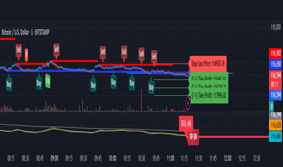
40 Ticker Cross-Sectional Z-Scores [BackQuant]40 Ticker Cross-Sectional Z-Scores
BackQuant’s 40 Ticker Cross-Sectional Z-Scores is a powerful portfolio management strategy that analyzes the relative performance of up to 40 different assets, comparing them on a cross-sectional basis to identify the top and bottom performers. This indicator computes Z-scores for each asset based on their log returns and evaluates them relative to the mean and standard deviation over a rolling window. The Z-scores represent how far an asset's return deviates from the average, and these values are used to rank the assets, allowing for dynamic asset allocation based on performance.
By focusing on the strongest-performing assets and avoiding the weakest, this strategy aims to enhance returns while managing risk. Additionally, by adjusting for standard deviations, the system offers a risk-adjusted method of ranking assets, making it suitable for traders who want to dynamically allocate capital based on performance metrics rather than just price movements.
Key Features
1. Cross-Sectional Z-Score Calculation:
The system calculates Z-scores for 40 different assets, evaluating their log returns against the mean and standard deviation over a rolling window. This enables users to assess the relative performance of each asset dynamically, highlighting which assets are performing better or worse compared to their historical norms. The Z-score is a useful statistical tool for identifying outliers in asset performance.
2. Asset Ranking and Allocation:
The system ranks assets based on their Z-scores and allocates capital to the top performers. It identifies the top and bottom assets, and traders can allocate capital to the top-performing assets, ensuring that their portfolio is aligned with the best performers. Conversely, the bottom assets are removed from the portfolio, reducing exposure to underperforming assets.
3. Rolling Window for Mean and Standard Deviation Calculations:
The Z-scores are calculated based on rolling means and standard deviations, making the system adaptive to changing market conditions. This rolling calculation window allows the strategy to adjust to recent performance trends and minimize the impact of outdated data.
4. Mean and Standard Deviation Visualization:
The script provides real-time visualizations of the mean (x̄) and standard deviation (σ) of asset returns, helping traders quickly identify trends and volatility in their portfolio. These visual indicators are useful for understanding the current market environment and making more informed allocation decisions.
5. Top & Bottom Performer Tables:
The system generates tables that display the top and bottom performers, ranked by their Z-scores. Traders can quickly see which assets are outperforming and underperforming. These tables provide clear and actionable insights, helping traders make informed decisions about which assets to include in their portfolio.
6. Customizable Parameters:
The strategy allows traders to customize several key parameters, including:
Rolling Calculation Window: Set the window size for the rolling mean and standard deviation calculations.
Top & Bottom Tickers: Choose how many of the top and bottom assets to display and allocate capital to.
Table Orientation: Select between vertical or horizontal table formats to suit the user’s preference.
7. Forward Test & Out-of-Sample Testing:
The system includes out-of-sample forward tests, ensuring that the strategy is evaluated based on real-time performance, not just historical data. This forward testing approach helps validate the robustness of the strategy in dynamic market conditions.
8. Visual Feedback and Alerts:
The system provides visual feedback on the current asset rankings and allocations, with dynamic labels and plots on the chart. Additionally, users receive alerts when allocations change, keeping them informed of important adjustments.
9. Risk Management via Z-Scores and Std Dev:
The system’s approach to asset selection is based on Z-scores, which normalize performance relative to the historical mean. By incorporating standard deviation, it accounts for the volatility and risk associated with each asset. This allows for more precise risk management and portfolio construction.
10. Note on Mean Reversion Strategy:
If you take the inverse of the signals provided by this indicator, the strategy can be used for mean-reversion rather than trend-following. This would involve buying the underperforming assets and selling the outperforming ones. However, it's important to note that this approach does not work well with highly correlated assets, as the relationship between the assets could result in the same directional movement, undermining the effectiveness of the mean-reversion strategy.
References
www.uts.edu.au
onlinelibrary.wiley.com
www.cmegroup.com
Final Thoughts
The 40 Ticker Cross-Sectional Z-Scores strategy offers a data-driven approach to portfolio management, dynamically allocating capital based on the relative performance of assets. By using Z-scores and standard deviations, this strategy ensures that capital is directed to the strongest performers while avoiding weaker assets, ultimately improving the risk-adjusted returns of the portfolio. Whether you’re focused on trend-following or looking to explore mean-reversion strategies, this flexible system can be tailored to suit your investment goals.
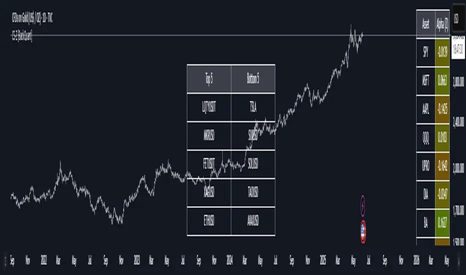
Gold Opening 15-Min ORB INDICATOR by AdéThis indicator is designed for trading Gold (XAUUSD) during the first 15 minutes of major market openings: Asian, European, and US sessions. It highlights these key time windows, plots the high and low ranges of each session, and generates breakout-based buy/sell signals. Ideal for traders focusing on volatility at market opens.
Features:Session Windows:
Asian: 1:00–1:15 AM Barcelona time (23:00–23:15 UTC, CEST-adjusted).
European: 9:00–9:15 AM Barcelona time (07:00–07:15 UTC).
US: 3:30–3:45 PM Barcelona time (13:30–13:45 UTC).
Marked with yellow (Asian), green (Europe), and blue (US) triangles below bars.
High/Low Ranges:Plots horizontal lines showing the highest high and lowest low of each session’s first 15 minutes.Lines appear after each session ends and persist until the next day, color-coded to match the sessions.Breakout Signals:Buy (Long): Triggers when the closing price breaks above the highest high of the previous 5 bars during a session window (lime triangle above bar).Sell (Short): Triggers when the closing price breaks below the lowest low of the previous 5 bars during a session window (red triangle below bar).
Signals are restricted to the 15-minute session periods for focused trading.Usage:Timeframe: Optimized for 1-minute XAUUSD charts.Timezone: Set your chart to UTC for accurate session timing (script uses UTC internally, based on Barcelona CEST, UTC+2 in April).Strategy:
Use buy/sell signals for breakout trades during volatile market opens, with session ranges as support/resistance levels.Customization: Adjust the lookback variable (default: 5) to tweak signal sensitivity.Notes:Tested for April 2025 (CEST, UTC+2).
Adjust timestamp values if using outside daylight saving time (CET, UTC+1) or for different broker timezones.Best for scalping or short-term trades during high-volatility periods. Combine with other indicators for confirmation if desired.How to Use:Apply to a 1-minute XAUUSD chart.Watch for session markers (triangles) and breakout signals during the 15-minute windows.Use the high/low lines to gauge potential breakout targets or reversals.

Poisson Projection of Price Levels### **Poisson Projection of Price Levels**
**Overview:**
The *Poisson Projection of Price Levels* is a cutting-edge technical indicator designed to identify and visualize potential support and resistance levels based on historical price interactions. By leveraging the Poisson distribution, this tool dynamically adjusts the significance of each price level's past "touches" to project future interactions with varying degrees of probability. This probabilistic approach offers traders a nuanced view of where price levels may hold or react in upcoming bars, enhancing both analysis and trading strategies.
---
**🔍 **Math & Methodology**
1. **Strata Levels:**
- **Definition:** Strata are horizontal lines spaced evenly around the current closing price.
- **Calculation:**
\
where \(i\) ranges from 0 to \(\text{Strata Count} - 1\).
2. **Forecast Iterations:**
- **Structure:** The indicator projects five forecast iterations into the future, each spaced by a Fibonacci sequence of bars: 2, 3, 5, 8, and 13 bars ahead. This spacing is inspired by the Fibonacci sequence, which is prevalent in financial market analysis for identifying key levels.
- **Purpose:** Each iteration represents a distinct forecast point where the price may interact with the strata, allowing for a multi-step projection of potential price levels.
3. **Touch Counting:**
- **Definition:** A "touch" occurs when the closing price of a bar is within half the increment of a stratum level.
- **Process:** For each stratum and each forecast iteration, the indicator counts the number of touches within a specified lookback window (e.g., 80 bars), offset by the forecasted position. This ensures that each iteration's touch count is independent and contextually relevant to its forecast horizon.
- **Adjustment:** Each forecast iteration analyzes a unique segment of the lookback window, offset by its forecasted position to ensure independent probability calculations.
4. **Poisson Probability Calculation:**
- **Formula:**
\
\
- **Interpretation:** \(p(k=1)\) represents the probability of exactly one touch occurring within the lookback window for each stratum and iteration.
- **Application:** This probability is used to determine the transparency of each stratum line, where higher probabilities result in more opaque (less transparent) lines, indicating stronger historical significance.
5. **Transparency Mapping:**
- **Calculation:**
\
- **Purpose:** Maps the Poisson probability to a visual transparency level, enhancing the readability of significant strata levels.
- **Outcome:** Strata with higher probabilities (more historical touches) appear more opaque, while those with lower probabilities appear fainter.
---
**📊 **Comparability to Standard Techniques**
1. **Support and Resistance Levels:**
- **Traditional Approach:** Traders identify support and resistance based on historical price reversals, pivot points, or psychological price levels.
- **Poisson Projection:** Automates and quantifies this process by statistically analyzing the frequency of price interactions with specific levels, providing a probabilistic measure of significance.
2. **Statistical Modeling:**
- **Standard Models:** Techniques like Moving Averages, Bollinger Bands, or Fibonacci Retracements offer dynamic and rule-based levels but lack direct probabilistic interpretation.
- **Poisson Projection:** Introduces a discrete event probability framework, offering a unique blend of statistical rigor and visual clarity that complements traditional indicators.
3. **Event-Based Analysis:**
- **Financial Industry Practices:** Event studies and high-frequency trading models often use Poisson processes to model order arrivals or price jumps.
- **Indicator Application:** While not identical, the use of Poisson probabilities in this indicator draws inspiration from event-based modeling, applying it to the context of price level interactions.
---
**💡 **Strengths & Advantages**
1. **Innovative Visualization:**
- Combines statistical probability with traditional support/resistance visualization, offering a fresh perspective on price level significance.
2. **Dynamic Adaptability:**
- Parameters like strata increment, lookback window, and probability threshold are user-defined, allowing customization across different markets and timeframes.
3. **Independent Probability Calculations:**
- Each forecast iteration calculates its own Poisson probability, ensuring that projections are contextually relevant and independent of other iterations.
4. **Clear Visual Cues:**
- Transparency-based coloring intuitively highlights significant price levels, making it easier for traders to identify key areas of interest at a glance.
---
**⚠️ **Limitations & Considerations**
1. **Poisson Assumptions:**
- Assumes that touches occur independently and at a constant average rate (\(\lambda\)), which may not always align with market realities characterized by trends and volatility clustering.
2. **Computational Intensity:**
- Managing multiple iterations and strata can be resource-intensive, potentially affecting performance on lower-powered devices or with very high lookback windows.
3. **Interpretation Complexity:**
- While transparency offers visual clarity, understanding the underlying probability calculations requires a basic grasp of Poisson statistics, which may be a barrier for some traders.
---
**📢 **How to Use It**
1. **Add to TradingView:**
- Open TradingView and navigate to the Pine Script Editor.
- Paste the script above and click **Add to Chart**.
2. **Configure Inputs:**
- **Strata Increment:** Set the desired price step between strata (e.g., `0.1` for 10 cents).
- **Lookback Window:** Define how many past bars to consider for calculating Poisson probabilities (e.g., `80`).
- **Probability Transparency Threshold (%):** Set the threshold percentage to map probabilities to line transparency (e.g., `25%`).
3. **Understand the Forecast Iterations:**
- The indicator projects five forecast points into the future at bar spacings of 2, 3, 5, 8, and 13 bars ahead.
- Each iteration independently calculates its Poisson probability based on the touch counts within its specific lookback window offset by its forecasted position.
4. **Interpret the Visualization:**
- **Opaque Lines:** Indicate higher Poisson probabilities, suggesting historically significant price levels that are more likely to interact again.
- **Fainter Lines:** Represent lower probabilities, indicating less historically significant levels that may be less likely to interact.
- **Forecast Spacing:** The spacing of 2, 3, 5, 8, and 13 bars ahead aligns with Fibonacci principles, offering a natural progression in forecast horizons.
5. **Apply to Trading Strategies:**
- **Support/Resistance Identification:** Use the opaque lines as potential support and resistance levels for placing trades.
- **Entry and Exit Points:** Anticipate price interactions at forecasted levels to plan strategic entries and exits.
- **Risk Management:** Utilize the transparency mapping to determine where to place stop-loss and take-profit orders based on the probability of price interactions.
6. **Customize as Needed:**
- Adjust the **Strata Increment** to fit different price ranges or volatility levels.
- Modify the **Lookback Window** to capture more or fewer historical touches, adapting to different timeframes or market conditions.
- Tweak the **Probability Transparency Threshold** to control the sensitivity of transparency mapping to Poisson probabilities.
**📈 **Practical Applications**
1. **Identifying Key Levels:**
- Quickly visualize which price levels have historically had significant interactions, aiding in the identification of potential support and resistance zones.
2. **Forecasting Price Reactions:**
- Use the forecast iterations to anticipate where price may interact in the near future, assisting in planning entry and exit points.
3. **Risk Management:**
- Determine areas of high probability for price reversals or consolidations, enabling better placement of stop-loss and take-profit orders.
4. **Market Analysis:**
- Assess the strength of market levels over different forecast horizons, providing a multi-layered understanding of market structure.
---
**🔗 **Conclusion**
The *Poisson Projection of Price Levels* bridges the gap between statistical modeling and traditional technical analysis, offering traders a sophisticated tool to quantify and visualize the significance of price levels. By integrating Poisson probabilities with dynamic transparency mapping, this indicator provides a unique and insightful perspective on potential support and resistance zones, enhancing both analysis and trading strategies.
---
**📞 **Contact:**
For support or inquiries, please contact me on TradingView!
---
**📢 **Join the Conversation!**
Have questions, feedback, or suggestions for further enhancements? Feel free to comment below or reach out directly. Your input helps refine and evolve this tool to better serve the trading community.
---
**Happy Trading!** 🚀

Aurum DCX AVE Gold and Silver StrategySummary in one paragraph
Aurum DCX AVE is a volatility break strategy for gold and silver on intraday and swing timeframes. It aligns a new Directional Convexity Index with an Adaptive Volatility Envelope and an optional USD/DXY bias so trades appear only when direction quality and expansion agree. It is original because it fuses three pieces rarely combined in one model for metals: a convexity aware trend strength score, a percentile based envelope that widens with regime heat, and an intermarket DXY filter.
Scope and intent
• Markets. Gold and silver futures or spot, other liquid commodities, major indices
• Timeframes. Five minutes to one day. Defaults to 30min for swing pace
• Default demo used in this publication. TVC:GOLD on 30m
• Purpose. Enter confirmed volatility breaks while muting chop using regime heat and USD bias
• Limits. This is a strategy. Orders are simulated on standard candles only
Originality and usefulness
• Unique fusion. DCX combines DI strength with path efficiency and curvature. AVE blends ATR with a high TR percentile and widens with DCX heat. DXY adds an intermarket bias
• Failure mode addressed. False starts inside compression and unconfirmed breakouts during USD swings
• Testability. Each component has a named input. Entry names L and S are visible in the list of trades
• Portable yardstick. Weekly ATR for stops and R multiples for targets
• Open source. Method and implementation are disclosed for community review
Method overview in plain language
You score direction quality with DCX, size an adaptive envelope with a blend of ATR and a high TR percentile, and only allow breaks that clear the band while DCX is above a heat threshold in the same direction. An optional DXY filter favors long when USD weakens and short when USD strengthens. Orders are bracketed with a Weekly ATR stop and an R multiple target, with optional trailing to the envelope.
Base measures
• Range basis. True Range and ATR over user windows. A high TR percentile captures expansion tails used by AVE
• Return basis. Not required
Components
• Directional Convexity Index DCX. Measures directional strength with DX, multiplies by path efficiency, blends a curvature term from acceleration, scales to 0 to 100, and uses a rise window
• Adaptive Volatility Envelope AVE. Midline ALMA or HMA or EMA plus bands sized by a blend of ATR and a high TR percentile. The blend weight follows volatility of volatility. Band width widens with DCX heat
• DXY Bias optional. Daily EMA trend of DXY. Long bias when USD weakens. Short bias when USD strengthens
• Risk block. Initial stop equals Weekly ATR times a multiplier. Target equals an R multiple of the initial risk. Optional trailing to AVE band
Fusion rule
• All gates must pass. DCX above threshold and rising. Directional lead agrees. Price breaks the AVE band in the same direction. DXY bias agrees when enabled
Signal rule
• Long. Close above AVE upper and DCX above threshold and DCX rising and plus DI leads and DXY bias is bearish
• Short. Close below AVE lower and DCX above threshold and DCX falling and minus DI leads and DXY bias is bullish
• Exit and flip. Bracket exit at stop or target. Optional trailing to AVE band
Inputs with guidance
Setup
• Symbol. Default TVC:GOLD (Correlation Asset for internal logic)
• Signal timeframe. Blank follows the chart
• Confirm timeframe. Default 1 day used by the bias block
Directional Convexity Index
• DCX window. Typical 10 to 21. Higher filters more. Lower reacts earlier
• DCX rise bars. Typical 3 to 6. Higher demands continuation
• DCX entry threshold. Typical 15 to 35. Higher avoids soft moves
• Efficiency floor. Typical 0.02 to 0.06. Stability in quiet tape
• Convexity weight 0..1. Typical 0.25 to 0.50. Higher gives curvature more influence
Adaptive Volatility Envelope
• AVE window. Typical 24 to 48. Higher smooths more
• Midline type. ALMA or HMA or EMA per preference
• TR percentile 0..100. Typical 75 to 90. Higher favors only strong expansions
• Vol of vol reference. Typical 0.05 to 0.30. Controls how much the percentile term weighs against ATR
• Base envelope mult. Typical 1.4 to 2.2. Width of bands
• Regime adapt 0..1. Typical 0.6 to 0.95. How much DCX heat widens or narrows the bands
Intermarket Bias
• Use DXY bias. Default ON
• DXY timeframe. Default 1 day
• DXY trend window. Typical 10 to 50
Risk
• Risk percent per trade. Reporting field. Keep live risk near one to two percent
• Weekly ATR. Default 14. Basis for stops
• Stop ATR weekly mult. Typical 1.5 to 3.0
• Take profit R multiple. Typical 1.5 to 3.0
• Trail with AVE band. Optional. OFF by default
Properties visible in this publication
• Initial capital. 20000
• Base currency. USD
• request.security lookahead off everywhere
• Commission. 0.03 percent
• Slippage. 5 ticks
• Default order size method percent of equity with value 3% of the total capital available
• Pyramiding 0
• Process orders on close ON
• Bar magnifier ON
• Recalculate after order is filled OFF
• Calc on every tick OFF
Realism and responsible publication
• No performance claims. Past results never guarantee future outcomes
• Shapes can move while a bar forms and settle on close
• Strategies use standard candles for signals and orders only
Honest limitations and failure modes
• Economic releases and thin liquidity can break assumptions behind the expansion logic
• Gap heavy symbols may prefer a longer ATR window
• Very quiet regimes can reduce signal contrast. Consider higher DCX thresholds or wider bands
• Session time follows the exchange of the chart and can change symbol to symbol
• Symbol sensitivity is expected. Use the gates and length inputs to find stable settings
Open source reuse and credits
• None
Mode
Public open source. Source is visible and free to reuse within TradingView House Rules
Legal
Education and research only. Not investment advice. You are responsible for your decisions. Test on historical data and in simulation before any live use. Use realistic costs.