OPR — DAX or USEnglish
This indicator automatically plots the Opening Price Range (OPR) for different indices, with customizable start and end times for each instrument.
For the DAX, it draws the high (green), low (red), and midline (grey dotted) for the specified range, defaulting to 09:00–09:15, and extends the lines until the selected end time (default 11:00).
For US indices (Dow Jones, Nasdaq, S&P500), it applies the same logic for the default 15:30–15:45 range, with two vertical black bars marking the start and end of the time window.
Each symbol only displays its own relevant lines (e.g., viewing DAX will only show DAX markers).
Parameters allow adjusting times and visibility for each market.
"机械革命无界15+时不时闪屏"に関するスクリプトを検索
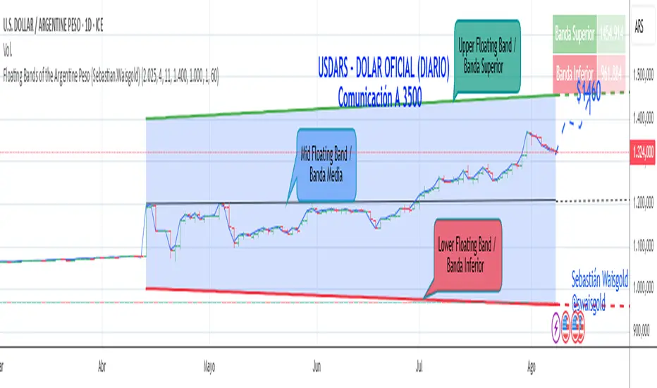
Floating Bands of the Argentine Peso (Sebastian.Waisgold)
The BCRA ( Central Bank of the Argentine Republic ) announced that as of Monday, April 15, 2025, the Argentine Peso (USDARS) will float within a system of divergent exchange rate bands.
The upper band was set at ARS 1400 per USD on 15/04/2025, with a +1% monthly adjustment distributed daily, rising by a fraction each day.
The lower band was set at ARS 1000 per USD on 15/04/2025, with a –1% monthly adjustment distributed daily, falling by a fraction each day.
This indicator is crucial for anyone trading USDARS, since the BCRA will only intervene in these situations:
- Selling : if the Peso depreciates against the USD above the upper band .
- Buying : if the Peso appreciates against the USD below the lower band .
Therefore, this indicator can be used as follows:
- If USDARS is above the upper band , it is “expensive” and you may sell .
- If USDARS is below the lower band , it is “cheap” and you may buy .
It can also be applied to other assets such as:
- USDTARS
- Dollar Cable / CCL (Contado con Liquidación) , derived from the BCBA:YPFD / NYSE:YPF ratio.
A mid band —exactly halfway between the upper and lower bands—has also been added.
Once added, the indicator should look like this:
In the following image you can see:
- Upper Floating Band
- Lower Floating Band
- Mid Floating Band
User Configuration
By double-clicking any line you can adjust:
- Start day (Dia de incio), month (Mes de inicio), and year (Año de inicio)
- Initial upper band value (Valor inicial banda superior)
- Initial lower band value (Valor inicial banda inferior)
- Monthly rate Tasa mensual %)
It is recommended not to modify these settings for the Argentine Peso, as they reflect the BCRA’s official framework. However, you may customize them—and the line colors—for other assets or currencies implementing a similar band scheme.
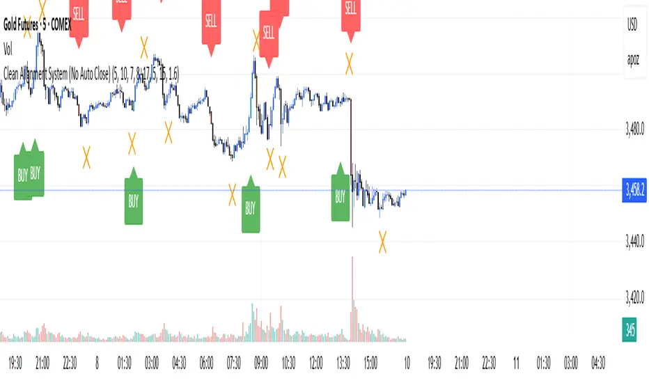
Clean Multi-Indicator Alignment System
Overview
A sophisticated multi-indicator alignment system designed for 24/7 trading across all markets, with pure signal-based exits and no time restrictions. Perfect for futures, forex, and crypto markets that operate around the clock.
Key Features
🎯 Multi-Indicator Confluence System
EMA Cross Strategy: Fast EMA (5) and Slow EMA (10) for precise trend direction
VWAP Integration: Institution-level price positioning analysis
RSI Momentum: 7-period RSI for momentum confirmation and reversal detection
MACD Signals: Optimized 8/17/5 configuration for scalping responsiveness
Volume Confirmation: Customizable volume multiplier (default 1.6x) for signal validation
🚀 Advanced Entry Logic
Initial Full Alignment: Requires all 5 indicators + volume confirmation
Smart Continuation Entries: EMA9 pullback entries when trend momentum remains intact
Flexible Time Controls: Optional session filtering or 24/7 operation
🎪 Pure Signal-Based Exits
No Forced Closes: Positions exit only on technical signal reversals
Dual Exit Conditions: EMA9 breakdown + RSI flip OR MACD cross + EMA20 breakdown
Trend Following: Allows profitable trends to run their full course
Perfect for Swing Scalping: Ideal for multi-session position holding
📊 Visual Interface
Real-Time Status Dashboard: Live alignment monitoring for all indicators
Color-Coded Candles: Instant visual confirmation of entry/exit signals
Clean Chart Display: Toggle-able EMAs and VWAP with professional styling
Signal Differentiation: Clear labels for entries, X-crosses for exits
🔔 Alert System
Entry Notifications: Separate alerts for buy/sell signals
Exit Warnings: Technical breakdown alerts for position management
Mobile Ready: Push notifications to TradingView mobile app
Market Applications
Perfect For:
Gold Futures (GC): 24-hour precious metals trading
NASDAQ Futures (NQ): High-volatility index scalping
Forex Markets: Currency pairs with continuous operation
Crypto Trading: 24/7 cryptocurrency momentum plays
Energy Futures: Oil, gas, and commodity swing trades
Optimal Timeframes:
1-5 Minutes: Ultra-fast scalping during high volatility
5-15 Minutes: Balanced approach for most markets
15-30 Minutes: Swing scalping for trend following
🧠 Smart Position Management
Tracks implied position direction
Prevents conflicting signals
Allows trend continuation entries
State-aware exit logic
⚡ Scalping Optimized
Fast-reacting indicators with shorter periods
Volume-based confirmation reduces false signals
Clean entry/exit visualization
Minimal lag for time-sensitive trades
Configuration Options
All parameters fully customizable:
EMA Lengths: Adjustable from 1-30 periods
RSI Period: 1-14 range for different market conditions
MACD Settings: Fast (1-15), Slow (1-30), Signal (1-10)
Volume Confirmation: 0.5-5.0x multiplier range
Visual Preferences: Colors, displays, and table options
Risk Management Features
Clear visual exit signals prevent emotion-based decisions
Volume confirmation reduces false breakouts
Multi-indicator confluence improves signal quality
Optional time filtering for session-specific strategies
Best Use Cases
Futures Scalping: NQ, ES, GC during active sessions
Forex Swing Trading: Major pairs during overlap periods
Crypto Momentum: Bitcoin, Ethereum trend following
24/7 Automated Systems: Algorithmic trading implementation
Multi-Market Scanning: Portfolio-wide signal monitoring
Opening Range BreakoutThis indicator is designed for Opening Range Breakout (ORB) traders who want automatic calculation of breakout levels and multiple price targets.
It is optimised for NSE intraday trading, capturing the first 15-minute range from 09:15 to 09:30 and plotting key breakout targets for both long and short trades.
✨ Features:
Automatic daily reset — fresh levels are calculated every trading day.
Opening Range High & Low plotted immediately after 09:30.
Two profit targets for both Buy & Sell breakouts based on the opening range size:
T1 = 100% of range added/subtracted from OR high/low.
T2 = 200% of range added/subtracted from OR high/low.
Clear breakout signals (BUY / SELL labels) when price crosses the OR High or Low.
Custom alerts for both buy and sell triggers.
Designed to work on any intraday timeframe (1min, 3min, 5min, etc.).
📊 How it works:
From 09:15 to 09:30, the script records the highest and lowest prices.
At 09:30, the range is locked in and breakout targets are calculated automatically.
Buy and Sell signals are generated when price breaks above the OR High or below the OR Low.
Targets and range lines automatically reset for the next day.
⚠️ Notes:
This script is tuned for NSE market timings but can be adapted for other markets by changing the session input.
Works best on intraday charts for active traders.
This is not financial advice — always backtest before trading live.

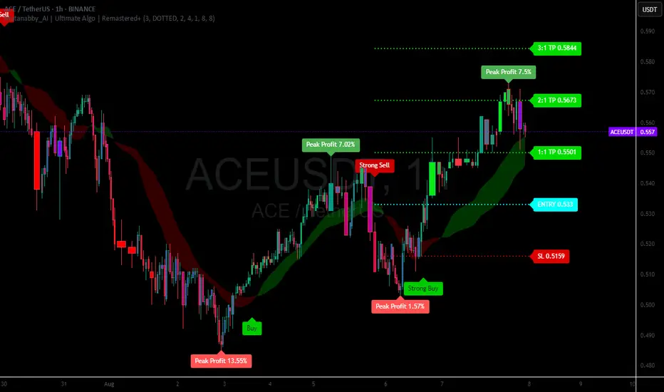
Mutanabby_AI | Ultimate Algo | Remastered+Overview
The Mutanabby_AI Ultimate Algo Remastered+ represents a sophisticated trend-following system that combines Supertrend analysis with multiple moving average confirmations. This comprehensive indicator is designed specifically for identifying high-probability trend continuation and reversal opportunities across various market conditions.
Core Algorithm Components
**Supertrend Foundation**: The primary signal generation relies on a customizable Supertrend indicator with adjustable sensitivity (1-20 range). This adaptive trend-following tool uses Average True Range calculations to establish dynamic support and resistance levels that respond to market volatility.
**SMA Confirmation Matrix**: Multiple Simple Moving Averages (SMA 4, 5, 9, 13) provide layered confirmation for signal strength. The algorithm distinguishes between regular signals and "Strong" signals based on SMA 4 vs SMA 5 relationship, offering traders different conviction levels for position sizing.
**Trend Ribbon Visualization**: SMA 21 and SMA 34 create a visual trend ribbon that changes color based on their relationship. Green ribbon indicates bullish momentum while red signals bearish conditions, providing immediate visual trend context.
**RSI-Based Candle Coloring**: Advanced 61-tier RSI system colors candles with gradient precision from deep red (RSI ≤20) through purple transitions to bright green (RSI ≥79). This visual enhancement helps traders instantly assess momentum strength and overbought/oversold conditions.
Signal Generation Logic
**Buy Signal Criteria**:
- Price crosses above Supertrend line
- Close price must be above SMA 9 (trend confirmation)
- Signal strength determined by SMA 4 vs SMA 5 relationship
- "Strong Buy" when SMA 4 ≥ SMA 5
- Regular "Buy" when SMA 4 < SMA 5
**Sell Signal Criteria**:
- Price crosses below Supertrend line
- Close price must be below SMA 9 (trend confirmation)
- Signal strength based on SMA relationship
- "Strong Sell" when SMA 4 ≤ SMA 5
- Regular "Sell" when SMA 4 > SMA 5
Advanced Risk Management System
**Automated TP/SL Calculation**: The indicator automatically calculates stop loss and take profit levels using ATR-based measurements. Risk percentage and ATR length are fully customizable, allowing traders to adapt to different market conditions and personal risk tolerance.
**Multiple Take Profit Targets**:
- 1:1 Risk-Reward ratio for conservative profit taking
- 2:1 Risk-Reward for balanced trade management
- 3:1 Risk-Reward for maximum profit potential
**Visual Risk Display**: All risk management levels appear as both labels and optional trend lines on the chart. Customizable line styles (solid, dashed, dotted) and positioning ensure clear visualization without chart clutter.
**Dynamic Level Updates**: Risk levels automatically recalculate with each new signal, maintaining current market relevance throughout position lifecycles.
Visual Enhancement Features
**Customizable Display Options**: Toggle trend ribbon, TP/SL levels, and risk lines independently. Decimal precision adjustments (1-8 decimal places) accommodate different instrument price formats and personal preferences.
**Professional Label System**: Clean, informative labels show entry points, stop losses, and take profit targets with precise price levels. Labels automatically position themselves for optimal chart readability.
**Color-Coded Momentum**: The gradient RSI candle coloring system provides instant visual feedback on momentum strength, helping traders assess market energy and potential reversal zones.
Implementation Strategy
**Timeframe Optimization**: The algorithm performs effectively across multiple timeframes, with higher timeframes (4H, Daily) providing more reliable signals for swing trading. Lower timeframes work well for day trading with appropriate risk adjustments.
**Sensitivity Adjustment**: Lower sensitivity values (1-5) generate fewer but higher-quality signals, ideal for conservative approaches. Higher sensitivity (15-20) increases signal frequency for active trading styles.
**Risk Management Integration**: Use the automated risk calculations as baseline parameters, adjusting risk percentage based on account size and market conditions. The 1:1, 2:1, 3:1 targets enable systematic profit-taking strategies.
Market Application
**Trend Following Excellence**: Primary strength lies in capturing significant trend movements through the Supertrend foundation with SMA confirmation. The dual-layer approach reduces false signals common in single-indicator systems.
**Momentum Assessment**: RSI-based candle coloring provides immediate momentum context, helping traders assess signal strength and potential continuation probability.
**Range Detection**: The trend ribbon helps identify ranging conditions when SMA 21 and SMA 34 converge, alerting traders to potential breakout opportunities.
Performance Optimization
**Signal Quality**: The requirement for both Supertrend crossover AND SMA 9 confirmation significantly improves signal reliability compared to basic trend-following approaches.
**Visual Clarity**: The comprehensive visual system enables rapid market assessment without complex calculations, ideal for traders managing multiple instruments.
**Adaptability**: Extensive customization options allow fine-tuning for specific markets, trading styles, and risk preferences while maintaining the core algorithm integrity.
## Non-Repainting Design
**Educational Note**: This indicator uses standard TradingView functions (Supertrend, SMA, RSI) with normal behavior patterns. Real-time updates on current candles are expected and standard across all technical indicators. Historical signals on closed candles remain fixed and unchanged, ensuring reliable backtesting and analysis.
**Signal Confirmation**: Final signals are confirmed only when candles close, following standard technical analysis principles. The algorithm provides clear distinction between developing signals and confirmed entries.
Technical Specifications
**Supertrend Parameters**: Default sensitivity of 4 with ATR length of 11 provides balanced signal generation. Sensitivity range from 1-20 allows adaptation to different market volatilities and trading preferences.
**Moving Average Configuration**: SMA periods of 8, 9, and 13 create multi-layered trend confirmation, while SMA 21 and 34 form the visual trend ribbon for broader market context.
**Risk Management**: ATR-based calculations with customizable risk percentage ensure dynamic adaptation to market volatility while maintaining consistent risk exposure principles.
Recommended Settings
**Conservative Approach**: Sensitivity 4-5, RSI length 14, higher timeframes (4H, Daily) for swing trading with maximum signal reliability.
**Active Trading**: Sensitivity 6-8, RSI length 8-10, intermediate timeframes (1H) for balanced signal frequency and quality.
**Scalping Setup**: Sensitivity 10-15, RSI length 5-8, lower timeframes (15-30min) with enhanced risk management protocols.
## Conclusion
The Mutanabby_AI Ultimate Algo Remastered+ combines proven trend-following principles with modern visual enhancements and comprehensive risk management. The algorithm's strength lies in its multi-layered confirmation approach and automated risk calculations, providing both novice and experienced traders with clear signals and systematic trade management.
Success with this system requires understanding the relationship between signal strength indicators and adapting sensitivity settings to match current market conditions. The comprehensive visual feedback system enables rapid decision-making while the automated risk management ensures consistent trade parameters.
Practice with different sensitivity settings and timeframes to optimize performance for your specific trading style and risk tolerance. The algorithm's systematic approach provides an excellent framework for disciplined trend-following strategies across various market environments.
ai quant oculusAI QUANT OCULUS
Version 1.0 | Pine Script v6
Purpose & Innovation
AI QUANT OCULUS integrates four distinct technical concepts—exponential trend filtering, adaptive smoothing, momentum oscillation, and Gaussian smoothing—into a single, cohesive system that delivers clear, objective buy and sell signals along with automatically plotted stop-loss and three profit-target levels. This mash-up goes beyond a simple EMA crossover or standalone TRIX oscillator by requiring confluence across trend, adaptive moving averages, momentum direction, and smoothed price action, reducing false triggers and focusing on high‐probability turning points.
How It Works & Why Its Components Matter
Trend Filter: EMA vs. Adaptive MA
EMA (20) measures the prevailing trend with fixed sensitivity.
Adaptive MA (also EMA-based, length 10) approximates a faster-responding moving average, standing in for a KAMA-style filter.
Bullish bias requires AMA > EMA; bearish bias requires AMA < EMA. This ensures signals align with both the underlying trend and a more nimble view of recent price action.
Momentum Confirmation: TRIX
Calculates a triple-smoothed EMA of price over TRIX Length (15), then converts it to a percentage rate-of-change oscillator.
Positive TRIX reinforces bullish entries; negative TRIX reinforces bearish entries. Using TRIX helps filter whipsaws by focusing on sustained momentum shifts.
Gaussian Price Smoother
Applies two back-to-back 5-period EMAs to the price (“gaussian” smoothing) to remove short-term noise.
Price above the smoothed line confirms strength for longs; below confirms weakness for shorts. This layer avoids entries on erratic spikes.
Confluence Signals
Buy Signal (isBull) fires only when:
AMA > EMA (trend alignment)
TRIX > 0 (momentum support)
Close > Gaussian (price strength)
Sell Signal (isBear) fires under the inverse conditions.
Requiring all three conditions simultaneously sharply reduces false triggers common to single-indicator systems.
Automatic Risk & Reward Plotting
On each new buy or sell signal (edge detection via not isBull or not isBear ), the script:
Stores entryPrice at the signal bar’s close.
Draws a stop-loss line at entry minus ATR(14) × Stop Multiplier (1.5) by default.
Plots three profit-target lines at entry plus ATR × Target Multiplier (1×, 1.5×, and 2×).
All previous labels and lines are deleted on each new signal, keeping the chart uncluttered and focusing only on the current trade.
Inputs & Customization
Input Description Default
EMA Length Period for the main trend EMA 20
Adaptive MA Length Period for the faster adaptive EM A substitute 10
TRIX Length Period for the triple-smoothed momentum oscillator 15
Dominant Cycle Length (Reserved) 40
Stop Multiplier ATR multiple for stop-loss distance 1.5
Target Multiplier ATR multiple for first profit target 1.5
Show Buy/Sell Signals Toggle on-chart labels for entry signals On
How to Use
Apply to Chart: Best on 15 m–1 h timeframes for swing entries or 5 m for agile scalps.
Wait for Full Confluence:
Look for the AMA to cross above/below the EMA and verify TRIX and Gaussian conditions on the same bar.
A bright “LONG” or “SHORT” label marks your entry.
Manage the Trade:
Place your stop where the red or green SL line appears.
Scale or exit at the three yellow TP1/TP2/TP3 lines, automatically drawn by volatility.
Repeat Cleanly: Each new signal clears prior annotations, ensuring you only track the active setup.
Why This Script Stands Out
Multi-Layer Confluence: Trend, momentum, and noise-reduction must all align, addressing the weaknesses of single-indicator strategies.
Automated Trade Management: No manual plotting—stop and target lines appear seamlessly with each signal.
Transparent & Customizable: All logic is open, adjustable, and clearly documented, allowing traders to tweak lengths and multipliers to suit different instruments.
Disclaimer
No indicator guarantees profit. Always backtest AI QUANT OCULUS extensively, combine its signals with your own analysis and risk controls, and practice sound money management before trading live.

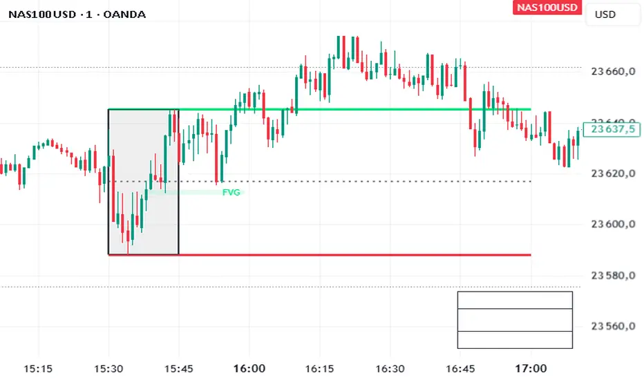
Pivot and Wick Boxes with Break Signals█ OVERVIEW
This Pine Script® indicator draws support and resistance levels based on high and low pivot points and the wicks of pivot candles. When the price breaks these levels, breakout signals are generated, with an optional volume filter for greater precision. The indicator is fully customizable, allowing users to adjust box styles, pivot length, and signal settings.
█ CONCEPTS
The indicator relies on several key elements to identify and visualize important price levels and trading signals:
Pivot Identification
High and low pivots are detected using the ta.pivothigh and ta.pivotlow functions with a configurable pivot length. Boxes are drawn based on the pivot level and the wick of the pivot candle (top for high pivots, bottom for low pivots).
List of Features
1 — High and Low Pivot Boxes: The indicator draws boxes based on high pivot candles (red) and low pivot candles (green) and their wicks, with options to customize colors, border styles, and background gradient. Boxes are limited to 500 bars back, meaning support and resistance levels older than 500 candles are not displayed to maintain chart clarity.
2 — Breakout Signals: When the price closes above the upper edge of a high pivot box, a breakout signal is generated (green triangle below the bar). When the price closes below the lower edge of a low pivot box, a breakout signal is generated (red triangle above the bar).
Signals can be filtered using volume, requiring the volume at the breakout to exceed the average volume multiplied by a configurable multiplier.
3 — Box Management: The indicator limits the number of displayed boxes (default is 15 for high pivots and 15 for low pivots), removing the oldest boxes when the limit is reached. Boxes older than 500 bars are automatically removed.
Volume Filtering
An optional volume filter allows users to require breakout signals to be confirmed by volume exceeding the moving average of volume (calculated over a selected period, default is 20 days).
█ OTHER SECTIONS
FEATURES
• Show High/Low Pivot Boxes: Enables or disables the display of boxes for high and low pivots.
• Pivot Length: Specifies the number of bars back and forward for detecting pivots (default is 5).
• Max Boxes: Sets the maximum number of boxes for high and low pivots (default is 15).
• Volume Filter: Enables a volume filter for breakout signals, with a configurable multiplier and average period.
• Box Style: Allows customization of border color, background gradient, border width, and border style (solid, dashed, dotted).
HOW TO USE
1 — Add the indicator to your TradingView chart by selecting “Pivot and Wick Boxes with Break Signals” from the indicators list.
2 — Configure the settings in the indicator’s dialog window, adjusting pivot length, maximum number of boxes, colors, and style.
3 — Enable the volume filter if you want signals to be confirmed by high volume.
4 — Monitor breakout signals (green triangles below bars for upward breakouts, red triangles above bars for downward breakouts) on the chart.
LIMITATIONS
• New pivots are detected with a delay equal to the set pivot length. A lower pivot length value results in faster pivot detection but produces pivots with less significance as support or resistance levels compared to those generated with a longer value.
• Breakout signals may produce false signals in volatile market conditions, especially without the volume filter.
• Boxes are limited to 500 bars back, which may exclude older pivots on long-term charts.

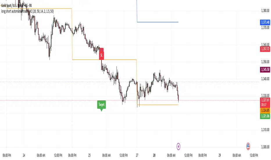
Momentum Reversal StrategyBEST USE IN 15MIN TIME FRAME EURUSD / XAUSUD
1. Strategy Overview
This strategy hunts short-term momentum reversals at key levels during high-liquidity sessions.
Timeframes: 5-minute for entries; 15-minute for trend context
Sessions: London for EUR/USD & GBP/USD; New York for XAU/USD
Pairs: EUR/USD, GBP/USD, XAU/USD
Indicators (3 max):
EMA(20) and EMA(50) (close)
MACD (12, 26, 9) histogram
Optional: RSI(14) (for divergence filter)
2. Entry Rules
Trend Filter (15 min):
Long only if EMA20 > EMA50; short only if EMA20 < EMA50.
Price-Action Zone (5 min):
Identify recent swing high/low within past 20 bars.
Draw horizontal support (for longs) or resistance (for shorts).
Indicator Alignment (5 min):
MACD histogram crossing from negative to positive for longs, positive to negative for shorts.
Candle close beyond EMA20 in direction of trade.
Candle Confirmation:
Bullish engulfing or hammer at support for longs; bearish engulfing or shooting star at resistance for shorts.
Entry Execution:
Place market order on candle close that meets all above.
3. Exit Rules
Stop-Loss (SL):
Long: 1.5× ATR(14) below entry candle low.
Short: 1.5× ATR(14) above entry candle high.
Take-Profit (TP):
Set at 2× SL distance (RR 1:2).
Trailing SL:
After price moves 1× SL in profit, trail SL to breakeven.
Partial Booking:
Close 50% at 1× SL (50% of TP), move SL to entry.
Close remaining at full TP.
4. Trade Management
False Signal Filter: Skip trades when RSI(14) > 70 for longs or < 30 for shorts (avoids overbought/oversold extremes).
One Trade at a Time: No multiple positions on same pair.
Session Cutoff: Close any open trade 15 minutes before session end.
5. Risk Parameters
Risk per Trade: 1% of account equity.
Reward Target: ≥2% (1:2 RR) per trade.
Win-Rate Expectancy: ≥75% based on indicator confluence and price-action confirmation.
Portfolio Tracker ARJO (V-01)Portfolio Tracker ARJO (V-01)
This indicator is a user-friendly portfolio tracking tool designed for TradingView charts. It overlays a customizable table on your chart to monitor up to 15 stocks or symbols in your portfolio. It calculates real-time metrics like current market price (CMP), gains/losses, and stoploss breaches, helping you stay on top of your investments without switching between multiple charts. The table uses color-coding for quick visual insights: green for profits, red for losses, and highlights breached stoplosses in red for alerts. It also shows portfolio-wide totals for overall performance.
Key Features
Supports up to 15 Symbols: Enter stock tickers (e.g., NSE:RELIANCE or BSE:TCS) with details like buy price, date, units, and stoploss.
Symbol: The stock ticker and description.
Buy Date: When you purchased it.
Units: Number of shares/units held.
Buy Price: Your entry price.
Stop Loss: Your set stoploss level (highlighted in red if breached by CMP).
CMP: Current market price (fetched from the chart's timeframe).
% Gain/Loss: Percentage change from buy price (color-coded: green for positive, red for negative).
Gain/Loss: Total monetary gain/loss based on units.
Optional Timeframe Columns: Toggle to show % change over 1 Week (1W), 1 Month (1M), 3 Months (3M), and 6 Months (6M) for historical performance.
Portfolio Summary: At the top of the table, see total % gain/loss and absolute gain/loss for your entire portfolio.
Visual Customizations: Adjust table position (e.g., Top Right), size, colors for positive/negative values, and intensity cutoff for gradients.
Benchmark Index-Based Header: The title row's background color reflects NIFTY's weekly trend (green if above 10-week SMA, red if below) for market context.
Benchmark Index-Based Header: The title row's background color reflects NIFTY's weekly trend (green if above 10-week SMA, red if below) for market context.
How to Use It: Step-by-Step Guide
Add the Indicator to Your Chart: Search for "Portfolio Tracker ARJO (V-01)" in TradingView's indicator library and add it to any chart (preferably Daily timeframe for accuracy).
Input Your Portfolio Symbols:
Open the indicator settings (gear icon).
In the "Symbol 1" to "Symbol 15" groups, fill in:
Symbol: Enter the ticker (e.g., NSE:INFY).
Year/Month/Day: Select your buy date (e.g., 2024-07-01).
Buy Price: Your purchase price per unit.
Stoploss: Your exit price if things go south.
Units: How many shares you own.
Only fill what you need—leave extras blank. The table auto-adjusts to show only entered symbols.
Customize the Table (Optional):
In "Table settings":
Choose position (e.g., Top Right) and size (% of chart).
Toggle "Show Timeframe Columns" to add 1W/1M/3M/6M performance.
In "Color settings":
Pick colors for positive (green) and negative (red) cells.
Set "Color intensity cutoff (%)" to control how strong the colors get (e.g., 10% means changes above 10% max out the color).
Interpret the Table on Your Chart:
The table appears overlaid—scan rows for each symbol's stats.
Look at colors: Greener = better gains; redder = bigger losses.
Check CMP cell: Red means stoploss breached—consider selling!
Portfolio Gain/Loss at the top gives a quick overall health check.
For Best Results:
Use on a Daily chart to avoid CMP errors (the script will warn if on Weekly/Monthly).
Refresh the chart or wait for a new bar if data doesn't update immediately.
For Indian stocks, prefix with NSE: or BSE: (e.g., BSE:RELIANCE).
This is for tracking only—not trading signals. Combine with your strategy.
If no symbols show, ensure inputs are valid (e.g., buy price > 0, valid date).
Finally, this tool makes it quite easy for beginners to track their portfolios, while also giving advanced traders powerful and customizable insights. I'd love to hear your feedback—happy trading!

Reversal Point Dynamics⇋ Reversal Point Dynamics (RPD)
This is not an indicator; it is a complete system for deconstructing the mechanics of a market reversal. Reversal Point Dynamics (RPD) moves far beyond simplistic pattern recognition, venturing into a deep analysis of the underlying forces that cause trends to exhaust, pause, and turn. It is engineered from the ground up to identify high-probability reversal points by quantifying the confluence of market dynamics in real-time.
Where other tools provide a static signal, RPD delivers a dynamic probability. It understands that a true market turning point is not a single event, but a cascade of failing momentum, structural breakdown, and a shift in market order. RPD's core engine meticulously analyzes each of these dynamic components—the market's underlying state, its velocity and acceleration, its degree of chaos (entropy), and its structural framework. These forces are synthesized into a single, unified Probability Score, offering you an unprecedented, transparent view into the conviction behind every potential reversal.
This is not a "black box" system. It is an open-architecture engine designed to empower the discerning trader. Featuring real-time signal projection, an integrated Fibonacci R2R Target Engine, and a comprehensive dashboard that acts as your Dynamics Control Center , RPD gives you a complete, holistic view of the market's state.
The Theoretical Core: Deconstructing Market Dynamics
RPD's analytical power is born from the intelligent synthesis of multiple, distinct theoretical models. Each pillar of the engine analyzes a different facet of market behavior. The convergence of these analyses—the "Singularity" event referenced in the dashboard—is what generates the final, high-conviction probability score.
1. Pillar One: Quantum State Analysis (QSA)
This is the foundational analysis of the market's current state within its recent context. Instead of treating price as a random walk, QSA quantizes it into a finite number of discrete "states."
Formulaic Concept: The engine establishes a price range using the highest high and lowest low over the Adaptive Analysis Period. This range is then divided into a user-defined number of Analysis Levels. The current price is mapped to one of these states (e.g., in a 9-level system, State 0 is the absolute low, and State 8 is the absolute high).
Analytical Edge: This acts as a powerful foundational filter. The engine will only begin searching for reversal signals when the market has reached a statistically stretched, extreme state (e.g., State 0 or 8). The Edge Sensitivity input allows you to control exactly how close to this extreme edge the price must be, ensuring you are trading from points of maximum potential exhaustion.
2. Pillar Two: Price State Roc (PSR) - The Dynamics of Momentum
This pillar analyzes the kinetic forces of the market: its velocity and acceleration. It understands that it’s not just where the price is, but how it got there that matters.
Formulaic Concept: The psr function calculates two derivatives of price.
Velocity: (price - price ). This measures the speed and direction of the current move.
Acceleration: (velocity - velocity ). This measures the rate of change in that speed. A negative acceleration (deceleration) during a strong rally is a critical pre-reversal warning, indicating momentum is fading even as price may be pushing higher.
Analytical Edge: The engine specifically hunts for exhaustion patterns where momentum is clearly decelerating as price reaches an extreme state. This is the mechanical signature of a weakening trend.
3. Pillar Three: Market Entropy Analysis - The Dynamics of Order & Chaos
This is RPD's chaos filter, a concept borrowed from information theory. Entropy measures the degree of randomness or disorder in the market's price action.
Formulaic Concept: The calculateEntropy function analyzes recent price changes. A market moving directionally and smoothly has low entropy (high order). A market chopping back and forth without direction has high entropy (high chaos). The value is normalized between 0 and 1.
Analytical Edge: The most reliable trades occur in low-entropy, ordered environments. RPD uses the Entropy Threshold to disqualify signals that attempt to form in chaotic, unpredictable conditions, providing a powerful shield against whipsaw markets.
4. Pillar Four: The Synthesis Engine & Probability Calculation
This is where all the dynamic forces converge. The final probability score is a weighted calculation that heavily rewards confluence.
Formulaic Concept: The calculateProbability function intelligently assembles the final score:
A Base Score is established from trend strength and entropy.
An Entropy Score adds points for low entropy (order) and subtracts for high entropy (chaos).
A significant Divergence Bonus is awarded for a classic momentum divergence.
RSI & Volume Bonuses are added if momentum oscillators are in extreme territory or a volume spike confirms institutional interest.
MTF & Adaptive Bonuses add further weight for alignment with higher timeframe structure.
Analytical Edge: A signal backed by multiple dynamic forces (e.g., extreme state + decelerating momentum + low entropy + volume spike) will receive an exponentially higher probability score. This is the very essence of analyzing reversal point dynamics.
The Command Center: Mastering the Inputs
Every input is a precise lever of control, allowing you to fine-tune the RPD engine to your exact trading style, market, and timeframe.
🧠 Core Algorithm
Predictive Mode (Early Detection):
What It Is: Enables the engine to search for potential reversals on the current, unclosed bar.
How It Works: Analyzes intra-bar acceleration and state to identify developing exhaustion. These signals are marked with a ' ? ' and are tentative.
How To Use It: Enable for scalping or very aggressive day trading to get the earliest possible indication. Disable for swing trading or a more conservative approach that waits for full bar confirmation.
Live Signal Mode (Current Bar):
What It Is: A highly aggressive mode that plots tentative signals with a ' ! ' on the live bar based on projected price and momentum. These signals repaint intra-bar.
How It Works: Uses a linear regression projection of the close to anticipate a reversal.
How To Use It: For advanced users who use intra-bar dynamics for execution and understand the nature of repainting signals.
Adaptive Analysis Period:
What It Is: The main lookback period for the QSA, PSR, and Entropy calculations. This is the engine's "memory."
How It Works: A shorter period makes the engine highly sensitive to local price swings. A longer period makes it focus only on major, significant market structure.
How To Use It: Scalping (1-5m): 15-25. Day Trading (15m-1H): 25-40. Swing Trading (4H+): 40-60.
Fractal Strength (Bars):
What It Is: Defines the strength of the pivot detection used for confirming reversal events.
How It Works: A value of '2' requires a candle's high/low to be more extreme than the two bars to its left and right.
How To Use It: '2' is a robust standard. Increase to '3' for an even stricter definition of a structural pivot, which will result in fewer signals.
MTF Multiplier:
What It Is: Integrates pivot data from a higher timeframe for confluence.
How It Works: A multiplier of '4' on a 15-minute chart will pull pivot data from the 1-hour chart (15 * 4 = 60m).
How To Use It: Set to a multiple that corresponds to your preferred higher timeframe for contextual analysis.
🎯 Signal Settings
Min Probability %:
What It Is: Your master quality filter. A signal is only plotted if its score exceeds this threshold.
How It Works: Directly filters the output of the final probability calculation.
How To Use It: High-Quality (80-95): For A+ setups only. Balanced (65-75): For day trading. Aggressive (50-60): For scalping.
Min Signal Distance (Bars):
What It Is: A noise filter that prevents signals from clustering in choppy conditions.
How It Works: Enforces a "cooldown" period of N bars after a signal.
How To Use It: Increase in ranging markets to focus on major swings. Decrease on lower timeframes.
Entropy Threshold:
What It Is: Your "chaos shield." Sets the maximum allowable market randomness for a signal.
How It Works: If calculated entropy is above this value, the signal is invalidated.
How To Use It: Lower values (0.1-0.5): Extremely strict. Higher values (0.7-1.0): More lenient. 0.85 is a good balance.
Adaptive Entropy & Aggressive Mode:
What It Is: Toggles for dynamically adjusting the engine's core parameters.
How It Works: Adaptive Entropy can slightly lower the required probability in strong trends. Aggressive Mode uses more lenient settings across the board.
How To Use It: Keep Adaptive on. Use Aggressive Mode sparingly, primarily for scalping highly volatile assets.
📊 State Analysis
Analysis Levels:
What It Is: The number of discrete "states" for the QSA.
How It Works: More levels create a finer-grained analysis of price location.
How To Use It: 6-7 levels are ideal. Increasing to 9 can provide more precision on very volatile assets.
Edge Sensitivity:
What It Is: Defines how close to the absolute top/bottom of the range price must be.
How It Works: '0' means price must be in the absolute highest/lowest state. '3' allows a signal within the top/bottom 3 states.
How To Use It: '3' provides a good balance. Lower it to '1' or '0' if you only want to trade extreme exhaustion.
The Dashboard: Your Dynamics Control Center
The dashboard provides a transparent, real-time view into the engine's brain. Use it to understand the context behind every signal and to gauge the current market environment at a glance.
🎯 UNIFIED PROB SCORE
TOTAL SCORE: The highest probability score (either Peak or Valley) the engine is currently calculating. This is your main at-a-glance conviction metric. The "Singularity" header refers to the event where market dynamics align—the event RPD is built to detect.
Quality: A human-readable interpretation of the Total Score. "EXCEPTIONAL" (🌟) is a rare, A+ confluence event. "STRONG" (💪) is a high-quality, tradable setup.
📊 ORDER FLOW & COMPONENT ANALYSIS
Volume Spike: Shows if the current volume is significantly higher than average (YES/NO). A 'YES' adds major confirmation.
Peak/Valley Conf: This breaks down the probability score into its directional components, showing you the separate confidence levels for a potential top (Peak) versus a bottom (Valley).
🌌 MARKET STRUCTURE
HTF Trend: Shows the direction of the underlying trend based on a Supertrend calculation.
Entropy: The current market chaos reading. "🔥 LOW" is an ideal, ordered state for trading. "😴 HIGH" is a warning of choppy, unpredictable conditions.
🔮 FIB & R2R ZONE (Large Dashboard)
This section gives you the status of the Fibonacci Target Engine. It shows if an Active Channel (entry zone) or Stop Zone (invalidation zone) is active and displays the precise price levels for the static entry, target, and stop calculated at the time of the signal.
🛡️ FILTERS & PREDICTIVES (Large Dashboard)
This panel provides a status check on all the bonus filters. It shows the current RSI Status, whether a Divergence is present, and if a Live Pending signal is forming.
The Visual Interface: A Symphony of Data
Every visual element is designed for instant, intuitive interpretation of market dynamics.
Signal Markers: These are the primary outputs of the engine.
▼/▲ b: A fully confirmed signal that has passed all filters.
? b: A tentative signal generated in Predictive Mode, indicating developing dynamics.
◈ b: This diamond icon replaces the standard triangle when the signal is confirmed by a strong momentum divergence, highlighting it as a superior setup where dynamics are misaligned with price.
Harmonic Wave: The flowing, colored wave around the price.
What It Represents: The market's "flow dynamic" and volatility.
How to Interpret It: Expanding waves show increasing volatility. The color is tied to the "Quantum Color" in your theme, representing the underlying energy field of the market.
Entropy Particles: The small dots appearing above/below price.
What They Represent: A direct visualization of the "order dynamic."
How to Interpret Them: Their presence signifies a low-entropy, ordered state ideal for trading. Their color indicates the direction of momentum (PSR velocity). Their absence means the market is too chaotic (high entropy).
The Fibonacci Target Engine: The dynamic R2R system appearing post-signal.
Static Fib Levels: Colored horizontal lines representing the market's "structural dynamic."
The Green "Active Channel" Box: Your zone of consideration. An area to manage a potential entry.
Development Philosophy
Reversal Point Dynamics was engineered to answer a fundamental question: can we objectively measure the forces behind a market turn? It is a synthesis of concepts from market microstructure, statistics, and information theory. The objective was never to create a "perfect" system, but to build a robust decision-support tool that provides a measurable, statistical edge by focusing on the principle of confluence.
By demanding that multiple, independent market dynamics align simultaneously, RPD filters out the vast majority of market noise. It is designed for the trader who thinks in terms of probability and risk management, not in terms of certainties. It is a tool to help you discount the obvious and bet on the unexpected alignment of market forces.
"Markets are constantly in a state of uncertainty and flux and money is made by discounting the obvious and betting on the unexpected."
— George Soros
Trade with insight. Trade with anticipation.
— Dskyz, for DAFE Trading Systems

Multi-Timeframe SMTSummery
The Multi-Timeframe SMT indicator is designed to identify and visualize Higher Timeframe (HTF) data on a Lower Timeframe (LTF) chart, allowing traders to see the broader market context without changing their current chart's resolution. It accurately draws pivots and SMT divergences from higher timeframes on the corresponding candles of your current lower timeframe chart.
Its core features include:
Multi-Timeframe Analysis: Configure and monitor pivots on up to four independent timeframes, from intraday to monthly.
Customizable Pivot Detection: Define the strength of pivots by adjusting the number of bars to the left and right.
SMT Divergence: Automatically identifies bullish and bearish SMT divergences by comparing the price action of the main chart symbol with a chosen correlated asset.
Early SMT Detection: A unique feature that monitors a lower "detection timeframe" to provide early warnings of potential SMT setups before they're confirmed on the main timeframe. Note that this early detection is only shown on timeframes equal to or lower than the "Detection timeframe" you have set.
Visual Cues & Alerts: Clear on-chart labels, lines, and fully customizable alerts notify you of confirmed pivots and SMT divergences, ensuring you don't miss key opportunities.
Important Nuance Regarding Pivot Label Display
Due to a self-imposed limit within this script's drawing management logic, the indicator might quickly reach its drawing capacity if you enable pivot crosses for multiple timeframes simultaneously. When this internal drawing limit is exceeded, the script is designed to automatically remove the oldest drawings to make space for new ones.
Therefore, to ensure optimal performance and visibility of the most recent and relevant pivots, it's highly recommended to only enable the "Show Pivot Crosses" option for one timeframe at a time. If you wish to view pivots for a different timeframe, simply disable the pivot crosses for the currently active timeframe and then enable them for your desired one. This approach prevents the rapid cycling and disappearance of pivot labels, providing a clearer and more stable visual experience.
In-Depth Explanation of the Logic
This script is built on two primary concepts: pivot points and Smart Money Technique (SMT) divergence. It systematically collects historical data on multiple timeframes, identifies pivots, and then compares them between two assets to find divergences.
Pivot Point Identification
A pivot is a turning point in the market. A pivot high is a candle that has a higher high than the candles to its immediate left and right. Conversely, a pivot low is a candle with a lower low than its neighbors.
How it Works in the Script:
The script tracks the highest high and lowest low for each period of the selected timeframe (e.g., for each 4-hour candle). When a new high-timeframe candle closes, it stores that high/low value and its bar index in an array. The checkForPivot() function then checks if a recently stored high or low qualifies as a pivot.
Key Inputs:
Left Strength (leftBars1): The number of candles to the left that must have a lower high (for a pivot high) or higher low (for a pivot low).
Right Strength (rightBars1): The number of candles to the right that must meet the same criteria.
For example, with Left Strength and Right Strength both set to 3, a pivot high is only confirmed when its high is greater than the highs of the 3 previous high-timeframe candles and the 3 subsequent high-timeframe candles. Increasing these values will identify more significant, longer-term pivots.
Smart Money Technique (SMT) Divergence
SMT Divergence is a concept popularized by The Inner Circle Trader (ICT). It occurs when two closely correlated assets fail to move in sync. For instance, if Asset A makes a higher high but Asset B fails to do so and instead makes a lower high, this creates a bearish SMT divergence. It suggests that the "smart money" may not be supporting the move in Asset A, signaling a potential reversal.
Bearish SMT: Main asset makes a higher high, while the correlated asset makes a lower high. This is a potential sell signal.
Bullish SMT: Main asset makes a lower low, while the correlated asset makes a higher low. This is a potential buy signal.
How it Works in the Script:
Data Request: For each timeframe, the script uses the request.security() function to fetch the high and low data for both the main chart symbol (syminfo.tickerid) and the chosen Comparison Asset.
Pivot Comparison: When a new pivot is confirmed on the main asset, the script checks if a corresponding pivot also formed on the comparison asset at the same time.
Divergence Check: It then compares the direction of the pivots. For a bearish SMT, it checks if the main asset's new pivot high is higher than its previous pivot high, while the comparison asset's new pivot high is lower than its previous one. The logic is reversed for bullish SMT.
Visualization: If a divergence is found, the script draws a red (bearish) or green (bullish) line connecting the two pivots on your chart and places an "SMT" label.
Early SMT Detection
This is a proactive feature designed to give you a heads-up. Waiting for a 4-hour or daily pivot to form can take a long time. The early detection system looks for SMT divergences on a much smaller, user-defined Detection timeframe (e.g., 15-minute).
How it Works in the Script:
Awaiting Setup: After a primary pivot (Pivot A) is formed on the main timeframe (e.g., a Daily pivot high), the script begins monitoring.
Intraday Monitoring: It then watches the Detection timeframe (e.g., 15-minute) for smaller intraday pivots.
Potential Divergence: It looks for an intraday pivot that forms a divergence against the primary Pivot A.
Watchline & Alert: When this "potential" divergence occurs, the script draws a dashed white line and triggers a "Potential SMT" alert. This isn't a confirmed SMT on the main timeframe yet, but it's a powerful early warning that one may be forming.
Drawing & Object Management
To keep the chart clean and prevent performance issues, the script manages its drawings (lines and labels) efficiently. It stores them in arrays and uses a drawing limit to automatically delete the oldest drawings as new ones are created, ensuring your TradingView remains responsive.
How to Use the Indicator
Configuration
Enable Timeframes: Use the checkboxes (Enable Timeframe 1, Enable Timeframe 2, etc.) to activate the timeframes you want to monitor. It's often best to start with one or two to keep the chart clean.
Select Timeframes: Choose the higher timeframes you want to analyze (e.g., 240 for 4-hour, D for Daily, W for Weekly).
Set Pivot Strength: The default of 3 for Left/Right strength is a good starting point. Increase it to find more significant market structure points or decrease it for more frequent, shorter-term pivots.
Configure SMT:
Check Enable SMT for the timeframes where you want to detect divergence.
Enter a Comparison Asset . This is crucial. Ensure the assets are correlated.
To use the early warning system, check Enable early SMT detection and select an appropriate Detection timeframe (e.g., 15 or 60 minutes for a Daily analysis).

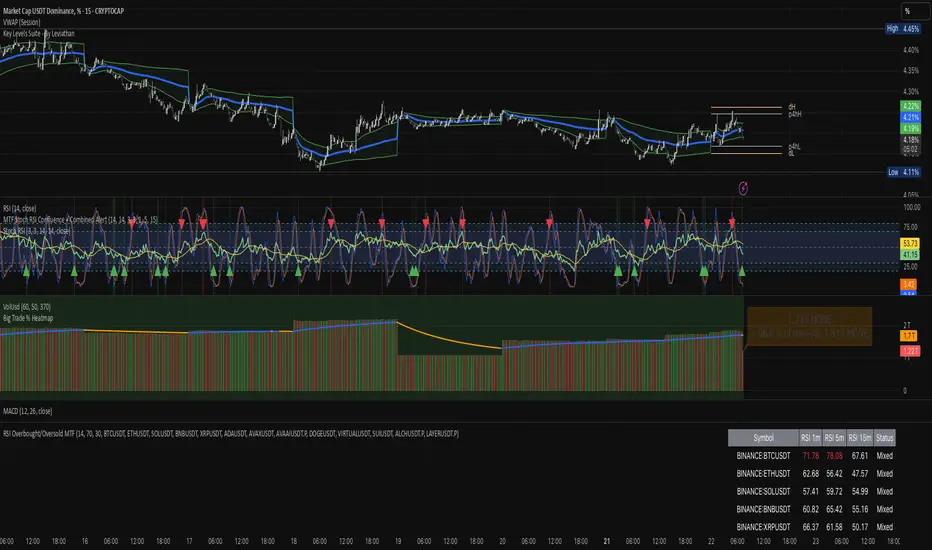
RSI Overbought/Oversold MTFRSI Overbought / Oversold MTF — Dashboard & Alerts
What it does
This script scans up to 13 symbols at once and shows their RSI readings on three lower‑time‑frames (1 min, 5 min, 15 min).
If all three RSIs for a symbol are simultaneously above the overbought threshold or below the oversold threshold, the script:
Prints the condition (“Overbought” / “Oversold”) in a color‑coded dashboard table.
Fires a one‑per‑bar alert so you never miss the move.
Key features
Feature Details
Multi‑symbol Default list includes BTC, ETH, SOL, BNB, XRP, ADA, AVAX, AVAAI, DOGE, VIRTUAL, SUI, ALCH, LAYER (all Binance pairs). Replace or reorder in the inputs.
Triple‑time‑frame check RSI is calculated on 1 m, 5 m, 15 m for each symbol.
Customizable thresholds Set your own RSI Period, Overbought and Oversold levels. Defaults: 14 / 70 / 30.
Color‑coded dashboard Top‑right table shows:
• Symbol name
• RSI 1 m / 5 m / 15 m (red = overbought, green = oversold, white = neutral)
• Overall Status column (“Overbought”, “Oversold”, “Mixed”).
Alerts built in Triggers once per bar whenever a symbol is overbought or oversold on all three time‑frames simultaneously.
Typical use cases
Scalp alignment — Enter when all short TFs agree on overbought/oversold extremes.
Mean‑reversion spotting — Identify stretched conditions across multiple coins without switching charts.
Quick sentiment scan — Glance at the dashboard to see where momentum is heating up or cooling down.
How to use
Add to chart (overlay = false; it sits in its own pane).
Adjust symbols & thresholds in the Settings panel.
Create alerts → choose “RSI Overbought/Oversold MTF” → “Any Alert() Function Call” to receive push, email, or webhook notifications.
Note: The script queries many symbols each bar; use on lower time‑frames only if your data limits allow.
For educational purposes only — not financial advice. Always test on paper before trading live.
Timeframe Quadrants | InvrsROBINHOODTimeframe Quadrant Visualizer
Summary
This indicator is a powerful visualization tool designed to help traders analyze price action by dividing various timeframes into four distinct, color-coded quadrants. By breaking down periods from a full year to a single minute, it offers a unique perspective on market cycles and intraday patterns. The script includes fully customizable colors and display styles, allowing you to tailor the visual output to your specific charting needs.
Key Features
Multiple Timeframe Divisions: Choose to divide a Year, Month, Week, Day, Hour, or Minute into four parts.
Customizable Quadrant Logic:
Year: Divided into calendar quarters (Jan-Mar, Apr-Jun, Jul-Sep, Oct-Dec).
Month: Divided into four approximate weeks (Days 1-7, 8-14, 15-21, 22-end).
Week: Divided into four 42-hour blocks, starting from Sunday at 00:00.
Day: Divided into four 6-hour blocks.
Hour: Divided into four 15-minute blocks.
Minute: Divided into four 15-second blocks.
Flexible Display Options: Visualize the quadrants as either a full Background Color overlay or a Bar Overlay that colors the price bars directly.
Timeframe Separators: A vertical line is automatically drawn at the beginning of each selected timeframe (e.g., at the start of each new day when "Day" is selected), making it easy to see where each period begins.
Full Color Customization: All four quadrant colors are user-definable, along with a global transparency setting to ensure the indicator complements your chart without obscuring price action.
Timezone-Aware: All calculations are performed based on a user-selected timezone from a dropdown menu, ensuring accuracy and consistency across different markets and trading sessions. As an added option, there is a manual input if the timezone is not available.
How to Use
Add to Chart: Add the "Timeframe Quadrants" indicator to your chart.
Open Settings: Hover over the indicator's name on your chart and click the Settings (gear) icon.
Configure the Indicator:
Timeframe: Select the primary time period you want to divide (e.g., "Day", "Week", "Hour").
Display Method: Choose whether you want the quadrants to appear as a Background Color or a Bar Overlay.
Timezone: Select the desired timezone from the dropdown menu. This is crucial for aligning the quadrants with specific market sessions (e.g., "America/New_York" for the NYSE session).
Quadrant Colors: Customize the color for each of the four quadrants.
Transparency %: Adjust the transparency of the colors to your preference.
Underlying Concepts
This script operates by using Pine Script's built-in time and date variables. It identifies the current bar's position within the user-selected timeframe (timeframe_choice) and assigns it to one of four quadrants based on pre-defined logic. For example, when "Day" is selected, it uses the hour() function to determine which 6-hour block the current bar falls into. The vertical separator lines are generated by detecting a change in the relevant time unit (e.g., ta.change(dayofmonth)), which marks the first bar of a new period.
Disclaimer: This tool is intended for visual analysis and pattern recognition. It does not generate buy or sell signals and should be used in conjunction with your own trading strategy and risk management. Past performance is not indicative of future results.

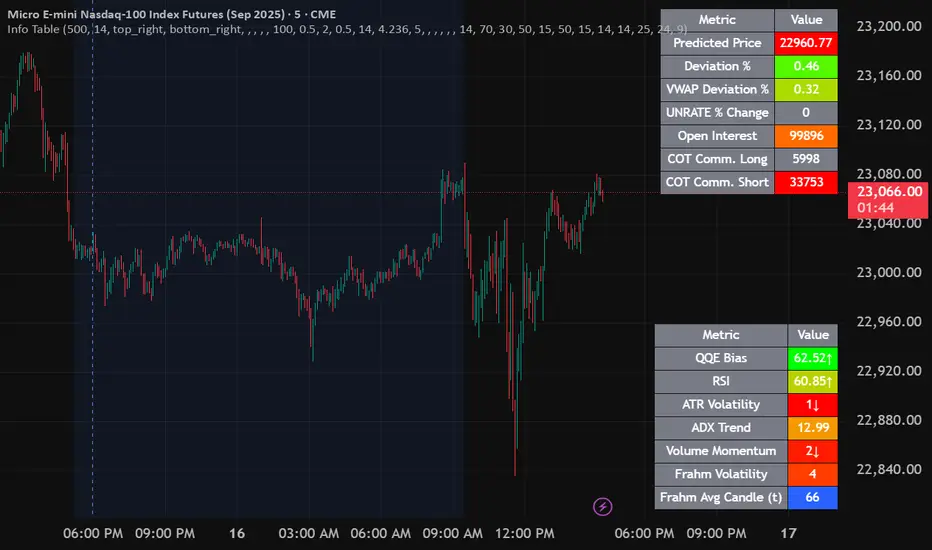
Info TableOverview
The Info Table V1 is a versatile TradingView indicator tailored for intraday futures traders, particularly those focusing on MESM2 (Micro E-mini S&P 500 futures) on 1-minute charts. It presents essential market insights through two customizable tables: the Main Table for predictive and macro metrics, and the New Metrics Table for momentum and volatility indicators. Designed for high-activity sessions like 9:30 AM–11:00 AM CDT, this tool helps traders assess price alignment, sentiment, and risk in real-time. Metrics update dynamically (except weekly COT data), with optional alerts for key conditions like volatility spikes or momentum shifts.
This indicator builds on foundational concepts like linear regression for predictions and adapts open-source elements for enhanced functionality. Gradient code is adapted from TradingView's Color Library. QQE logic is adapted from LuxAlgo's QQE Weighted Oscillator, licensed under CC BY-NC-SA 4.0. The script is released under the Mozilla Public License 2.0.
Key Features
Two Customizable Tables: Positioned independently (e.g., top-right for Main, bottom-right for New Metrics) with toggle options to show/hide for a clutter-free chart.
Gradient Coloring: User-defined high/low colors (default green/red) for quick visual interpretation of extremes, such as overbought/oversold or high volatility.
Arrows for Directional Bias: In the New Metrics Table, up (↑) or down (↓) arrows appear in value cells based on metric thresholds (top/bottom 25% of range), indicating bullish/high or bearish/low conditions.
Consensus Highlighting: The New Metrics Table's title cells ("Metric" and "Value") turn green if all arrows are ↑ (strong bullish consensus), red if all are ↓ (strong bearish consensus), or gray otherwise.
Predicted Price Plot: Optional line (default blue) overlaying the ML-predicted price for visual comparison with actual price action.
Alerts: Notifications for high/low Frahm Volatility (≥8 or ≤3) and QQE Bias crosses (bullish/bearish momentum shifts).
Main Table Metrics
This table focuses on predictive, positional, and macro insights:
ML-Predicted Price: A linear regression forecast using normalized price, volume, and RSI over a customizable lookback (default 500 bars). Gradient scales from low (red) to high (green) relative to the current price ± threshold (default 100 points).
Deviation %: Percentage difference between current price and predicted price. Gradient highlights extremes (±0.5% default threshold), signaling potential overextensions.
VWAP Deviation %: Percentage difference from Volume Weighted Average Price (VWAP). Gradient indicates if price is above (green) or below (red) fair value (±0.5% default).
FRED UNRATE % Change: Percentage change in U.S. unemployment rate (via FRED data). Cell turns red for increases (economic weakness), green for decreases (strength), gray if zero or disabled.
Open Interest: Total open MESM2 futures contracts. Gradient scales from low (red) to high (green) up to a hardcoded 300,000 threshold, reflecting market participation.
COT Commercial Long/Short: Weekly Commitment of Traders data for commercial positions. Long cell green if longs > shorts (bullish institutional sentiment); Short cell red if shorts > longs (bearish); gray otherwise.
New Metrics Table Metrics
This table emphasizes technical momentum and volatility, with arrows for quick bias assessment:
QQE Bias: Smoothed RSI vs. trailing stop (default length 14, factor 4.236, smooth 5). Green for bullish (RSI > stop, ↑ arrow), red for bearish (RSI < stop, ↓ arrow), gray for neutral.
RSI: Relative Strength Index (default period 14). Gradient from oversold (red, <30 + threshold offset, ↓ arrow if ≤40) to overbought (green, >70 - offset, ↑ arrow if ≥60).
ATR Volatility: Score (1–20) based on Average True Range (default period 14, lookback 50). High scores (green, ↑ if ≥15) signal swings; low (red, ↓ if ≤5) indicate calm.
ADX Trend: Average Directional Index (default period 14). Gradient from weak (red, ↓ if ≤0.25×25 threshold) to strong trends (green, ↑ if ≥0.75×25).
Volume Momentum: Score (1–20) comparing current to historical volume (lookback 50). High (green, ↑ if ≥15) suggests pressure; low (red, ↓ if ≤5) implies weakness.
Frahm Volatility: Score (1–20) from true range over a window (default 24 hours, multiplier 9). Dynamic gradient (green/red/yellow); ↑ if ≥7.5, ↓ if ≤2.5.
Frahm Avg Candle (Ticks): Average candle size in ticks over the window. Blue gradient (or dynamic green/red/yellow); ↑ if ≥0.75 percentile, ↓ if ≤0.25.
Arrows trigger on metric-specific logic (e.g., RSI ≥60 for ↑), providing directional cues without strict color ties.
Customization Options
Adapt the indicator to your strategy:
ML Inputs: Lookback (10–5000 bars) and RSI period (2+) for prediction sensitivity—shorter for volatility, longer for trends.
Timeframes: Individual per metric (e.g., 1H for QQE Bias to match higher frames; blank for chart timeframe).
Thresholds: Adjust gradients and arrows (e.g., Deviation 0.1–5%, ADX 0–100, RSI overbought/oversold).
QQE Settings: Length, factor, and smooth for fine-tuned momentum.
Data Toggles: Enable/disable FRED, Open Interest, COT for focus (e.g., disable macro for pure intraday).
Frahm Options: Window hours (1+), scale multiplier (1–10), dynamic colors for avg candle.
Plot/Table: Line color, positions, gradients, and visibility.
Ideal Use Case
Perfect for MESM2 scalpers and trend traders. Use the Main Table for entry confirmation via predicted deviations and institutional positioning. Leverage the New Metrics Table arrows for short-term signals—enter bullish on green consensus (all ↑), avoid chop on low volatility. Set alerts to catch shifts without constant monitoring.
Why It's Valuable
Info Table V1 consolidates diverse metrics into actionable visuals, answering critical questions: Is price mispriced? Is momentum aligning? Is volatility manageable? With real-time updates, consensus highlights, and extensive customization, it enhances precision in fast markets, reducing guesswork for confident trades.
Note: Optimized for futures; some metrics (OI, COT) unavailable on non-futures symbols. Test on demo accounts. No financial advice—use at your own risk.
The provided script reuses open-source elements from TradingView's Color Library and LuxAlgo's QQE Weighted Oscillator, as noted in the script comments and description. Credits are appropriately given in both the description and code comments, satisfying the requirement for attribution.
Regarding significant improvements and proportion:
The QQE logic comprises approximately 15 lines of code in a script exceeding 400 lines, representing a small proportion (<5%).
Adaptations include integration with multi-timeframe support via request.security, user-customizable inputs for length, factor, and smooth, and application within a broader table-based indicator for momentum bias display (with color gradients, arrows, and alerts). This extends the original QQE beyond standalone oscillator use, incorporating it as one of seven metrics in the New Metrics Table for confluence analysis (e.g., consensus highlighting when all metrics align). These are functional enhancements, not mere stylistic or variable changes.
The Color Library usage is via official import (import TradingView/Color/1 as Color), leveraging built-in gradient functions without copying code, and applied to enhance visual interpretation across multiple metrics.
The script complies with the rules: reused code is minimal, significantly improved through integration and expansion, and properly credited. It qualifies for open-source publication under the Mozilla Public License 2.0, as stated.
Staccked SMA - Regime Switching & Persistance StatisticsThis indicator is designed to identify the prevailing market regime by analyzing the behavior of a "stack" of Simple Moving Averages (SMAs). It helps you understand whether the market is currently trending, mean-reverting, or moving randomly.
Core Concept: SMA Correlation
At its heart, the indicator examines the relationship between a set of nine SMAs with different lengths (3, 5, 8, 13, 21, 34, 55, 89, 144) and the lengths themselves.
In a strong trending market (either up or down), the SMAs will be neatly "stacked" in order of their length. The shortest SMA will be furthest from the longest SMA, creating a strong, almost linear visual pattern. When we measure the statistical correlation between the SMA values and their corresponding lengths, we get a value close to +1 (perfect uptrend stack) or -1 (perfect downtrend stack). The absolute value of this correlation will be very high (close to 1).
In a mean-reverting or sideways market, the SMAs will be tangled and crisscrossing each other. There is no clear order, and the relationship between an SMA's length and its price value is weak. The correlation will be close to 0.
This indicator calculates this Pearson correlation on every bar, giving a continuous measure of how ordered or "trendy" the SMAs are. An absolute correlation above 0.8 is considered strongly trending, while a value between 0.4 and 0.8 suggests a mean-reverting character. Below 0.4, the market is likely random or choppy.
Regime Classification and Statistics
The indicator doesn't just look at the current correlation; it analyzes its behavior over a user-defined lookback window (default is 252 bars) to classify the overall market "regime."
It presents its findings in a clear table:
📊 |SMA Correlation| Regime Table: This main table provides a snapshot of the current market character.
Median: Shows the median absolute correlation over the lookback period, giving a central tendency of the market's behavior.
% > 0.80: The percentage of time the market was in a strong trend during the lookback period.
% < 0.80 & > 0.40: The percentage of time the market showed mean-reverting characteristics.
🧠 Regime: The final classification. It's labeled "📈 Trend-Dominant" if the median correlation is high and it has spent a significant portion of the time trending. It's labeled "🔄 Mean-Reverting" if the median is in the middle range and it has spent significant time in that state. Otherwise, it's considered "⚖️ Random/ Choppy".
📐 Regime Significance: This tells you how statistically confident you can be in the current regime classification, using a Z-score to compare its occurrence against random chance. ⭐⭐⭐ indicates high confidence (99%), while "❌ Not Significant" means the pattern could be random.
Regime Transition Probabilities
Optionally, a second table can be displayed that shows the historical probability of the market transitioning from one regime to another over different time horizons (t+5, t+10, t+15, and t+20 bars).
📈 → 🔄 → ⚖️ Transition Table: This table answers questions like, "If the market is trending now (From: 📈), what is the probability it will be mean-reverting (→ 🔄) in 10 bars?"
This provides powerful insights into the market's cyclical nature, helping you anticipate future behavior based on past patterns. For example, you might find that after a period of strong trending, a transition to a choppy state is more likely than a direct switch to a mean-reverting
Indicator Settings
Lookback Window for Regime Classification: This sets the number of recent bars (default is 252) the script analyzes to determine the current market regime (Trending, Mean-Reverting, or Random). A larger number provides a more stable, long-term view, while a smaller number makes the classification more sensitive to recent price action.
Show Regime Transition Table: A simple toggle (on/off) to show or hide the table that displays the probabilities of the market switching from one regime to another.
Lookback Offset for Starting Regime: This determines the "starting point" in the past for calculating regime transitions. The default is 20 bars ago. The script looks at the regime at this point and then checks what it became at later points.
Step 1, 2, 3, 4 Offset (bars): These define the future time intervals (5, 10, 15, and 20 bars by default) for the transition probability table. For example, the script checks the regime at the "Lookback Offset" and then sees what it transitioned to 5, 10, 15, and 20 bars later.
Significance Filter Settings
Use Regime Significance Filter: When enabled, this filter ensures that the regime transition statistics only count transitions that were "statistically significant." This helps to filter out noise and focus on more reliable patterns.
Min Stars Required (1=90%, 2=95%, 3=99%): This sets the minimum confidence level required for a regime to be included in the transition statistics when the significance filter is on.
1 ⭐: Requires at least 90% confidence.
2 ⭐⭐: Requires at least 95% confidence (default).
3 ⭐⭐⭐: Requires at least 99% confidence.

Smart Directional Fib Zone (Selectable Session)🎯 Overview
This indicator plots a dynamic Fibonacci zone between the 0.5 and 0.618 levels , calculated from the previous day’s price action , and is designed specifically for intraday traders.
It visually highlights key retracement or reaction areas where the market often pauses or reverses.
🔍 How it works
At the start of each day, the script automatically captures:
the previous day’s open (pdo),
high (pdh),
low (pdl),
and close (pdc).
It then determines if the previous day was bullish (Close > Open) or bearish (Close < Open).
Based on that:
If the previous day was bullish, it projects the Fibonacci levels down from the high (typical for expecting retracements).
If bearish, it projects them up from the low.
The two key levels are:
0.5 (50%) retracement / projection
0.618 (61.8%) retracement / projection
A colored zone is plotted between these levels to act as a leading guide for intraday setups.
⏰ Time filtering & session customization
A unique feature is the dynamic session filtering:
By default, the zone is only plotted during active market hours, keeping your chart clean outside trading hours.
The script provides a dropdown selector so you can quickly switch between:
India session (9:15 to 15:30)
Europe session (9:00 to 17:30)
US session (9:30 to 16:00)
Or even define your own custom session times.
This makes it ideal for intraday traders in any region.
🎨 Visual features
The fill zone changes color based on the previous day’s sentiment:
Green zone if the previous day was bullish
Red zone if the previous day was bearish
🚨 Alerts
The script includes an alert condition, so you can easily set up TradingView alerts to notify you when:
Price enters the Fibonacci zone.
This is extremely helpful for catching retracements or reversals without staring at the screen all day.
⚙️ How to use
✅ Works on any intraday timeframe (1 min, 5 min, 15 min, etc.).
✅ Simply add it to your chart, pick your session in the dropdown, and watch the Fibonacci zone automatically adjust to your selected market hours.
Use it as a confluence tool alongside other indicators like VWAP, EMAs, Bollinger Bands, or price action patterns to time entries and exits.
💪 Why this is powerful
This is more than a simple Fib retracement tool:
It dynamically adapts to the previous day’s sentiment, helping you trade in alignment with recent market psychology.
The session filtering ensures your charts are focused only on the periods

GeeksDoByte 15m & 30m ORB + Prev Day High/LowCME_MINI:NQ1!
How It Works
Opening Ranges
At 9:30 ET, the script begins tracking the high & low.
It uses two fixed sessions:
15 min from 09:30 to 09:45
30 min from 09:30 to 10:00
On the very first bar of each session it initializes the range, then continuously updates the high/low on each new intraday bar.
Dashed lines are drawn when the session opens and extended horizontally across subsequent bars.
Previous Day’s Levels
Independently, it fetches yesterday’s high and low via a daily security call.
These historic levels are plotted as simple horizontal lines for daily context.
How to Use
Breakout Entries
A close above the 15 min ORB high can signal an early breakout; a further push above the 30 min ORB high confirms extended momentum.
Conversely, breaks below the respective lows can indicate short setups.
Support & Resistance
Yesterday’s high/low often act as magnet levels. If price is near the previous high when the opening ranges break, you get a confluence zone worth watching.
Trade Management
Combine the two opening-range levels to tier your stops or scale in.
For example, you might place an initial stop below the 15 min low and a wider stop below the 30 min low.

LVN/HVN Auto Detection [PhenLabs]📊 PhenLabs - LVN/HVN Auto Detection
Version: PineScript™ v6
📌 Description
The PhenLabs LVN/HVN Auto Detection indicator is an advanced volume profile analysis tool that automatically identifies Low Volume Nodes (LVN) and High Volume Nodes (HVN) across multiple trading sessions. This sophisticated indicator analyzes volume distribution patterns to pinpoint critical support and resistance levels where price is likely to react, providing traders with high-probability zones for entries, exits, and risk management.
Unlike traditional volume indicators that only show current activity, this tool builds comprehensive volume profiles from historical sessions and intelligently filters the most significant levels. It combines real-time volume analysis with dynamic level detection, offering both visual bubbles for immediate volume activity and persistent horizontal lines that act as ongoing support/resistance references.
🚀 Points of Innovation
Multi-Session Volume Profile Analysis - Automatically calculates and analyzes volume profiles across the last 5 trading sessions
Intelligent Level Separation Logic - Prevents overlapping signals by maintaining minimum separation between LVN and HVN levels
Dynamic Timeframe Adaptation - Automatically adjusts session lengths based on chart timeframe for optimal level detection
Real-Time Activity Bubbles - Shows volume activity strength through different bubble sizes at key levels
Persistent Line Management - Creates horizontal lines that extend until price crosses them, providing ongoing reference points
Dual Threshold System - Independent percentage-based thresholds for both LVN and HVN identification
🔧 Core Components
Volume Profile Engine : Builds 20-row volume profiles for each analyzed session, distributing volume across price levels
Level Identification Algorithm : Uses percentage-based thresholds to classify volume distribution patterns
Separation Logic : Ensures minimum distance between conflicting levels, prioritizing HVN when overlap occurs
Line Management System : Tracks active support/resistance lines and removes them when price crosses through
Volume Activity Monitor : Compares current volume to 13-period moving average for activity classification
🔥 Key Features
Customizable Thresholds : LVN threshold (5-35%, default 20%) and HVN threshold (65-95%, default 80%) for precise level filtering
Volume Activity Multiplier : Adjustable volume threshold (0.5+, default 1.5) for bubble and line creation sensitivity
Flexible Display Modes : Choose between Lines only, Bubbles only, or Both for optimal chart clarity
Smart Level Separation : Minimum separation percentage (0.1-2%, default 0.5%) prevents conflicting signals
Color Customization : Independent color controls for LVN (red) and HVN (blue) elements
Performance Optimization : Processes every 15 bars with maximum 500 active lines for smooth operation
🎨 Visualization
Colored Bubbles : Three sizes (large, medium, small) indicate volume activity strength at key levels
Horizontal Lines : Persistent support/resistance lines with width corresponding to volume activity
Dual Color System : Semi-transparent red for LVN areas, semi-transparent blue for HVN zones
Information Tooltip : Optional table showing usage guidelines and optimization tips
📖 Usage Guidelines
Volume Thresholds
LVN Threshold
○ Default: 20.0%
○ Range: 5.0-35.0%
○ Description: Price levels with volume below this percentage are marked as LVNs. Lower values create fewer, more significant levels. Typical range 15-25% works for most instruments.
HVN Threshold
○ Default: 80.0%
○ Range: 65.0-95.0%
○ Description: Price levels with volume above this percentage are marked as HVNs. Higher values create fewer, stronger levels. Range 75-85% is optimal for most trading.
Display Controls
Volume Threshold
○ Default: 1.5
○ Range: 0.5+
○ Description: Multiplier for volume significance (High=2+threshold, Medium=1+threshold, Low=0+threshold). Higher values require more volume for signals.
✅ Best Use Cases
Swing Trading : Identify key levels for position entries and exits over multiple days
Scalping : Use bubbles for immediate volume activity confirmation at critical levels
Risk Management : Place stops beyond LVN levels where price moves quickly
Breakout Trading : Monitor HVN levels for potential breakout or rejection scenarios
Multi-Timeframe Analysis : Combine with higher timeframe levels for confluence
⚠️ Limitations
Timeframe Sensitivity : Lower timeframes may produce too many levels; higher timeframes recommended for cleaner signals
Volume Data Dependency : Accuracy depends on reliable volume data from your data provider
Historical Analysis : Uses past volume data which may not predict future price behavior
Performance Impact : High number of active lines may affect chart performance on slower devices
💡 What Makes This Unique
Automated Session Analysis : No manual drawing required - automatically analyzes multiple sessions
Intelligent Filtering : Advanced separation logic prevents overlapping and conflicting signals
Adaptive Processing : Adjusts to different timeframes automatically for optimal level detection
Dual Visualization System : Combines persistent lines with real-time activity indicators
🔬 How It Works
1. Volume Profile Construction :
Analyzes the last 5 trading sessions with dynamic session length based on timeframe
Divides each session’s price range into 20 equal levels for volume distribution analysis
2. Level Classification :
Calculates volume percentage at each price level relative to session maximum
Identifies LVN levels below threshold and HVN levels above threshold
3. Signal Generation :
Creates bubbles when volume activity exceeds thresholds at identified levels
Draws horizontal lines that persist until price crosses through them
💡 Note : For optimal results, increase your chart timeframe if you see too many levels. The indicator performs best on 15-minute and higher timeframes where volume patterns are more meaningful and less noisy.

Canuck Trading Trader StrategyCanuck Trading Trader Strategy
Overview
The Canuck Trading Trader Strategy is a high-performance, trend-following trading system designed for NASDAQ:TSLA on a 15-minute timeframe. Optimized for precision and profitability, this strategy leverages short-term price trends to capture consistent gains while maintaining robust risk management. Ideal for traders seeking an automated, data-driven approach to trading Tesla’s volatile market, it delivers strong returns with controlled drawdowns.
Key Features
Trend-Based Entries: Identifies short-term trends using a 2-candle lookback period and a minimum trend strength of 0.2%, ensuring responsive trade signals.
Risk Management: Includes a configurable 3.0% stop-loss to cap losses and a 2.0% take-profit to lock in gains, balancing risk and reward.
High Precision: Utilizes bar magnification for accurate backtesting, reflecting realistic trade execution with 1-tick slippage and 0.1 commission.
Clean Interface: No on-chart indicators, providing a distraction-free trading experience focused on performance.
Flexible Sizing: Allocates 10% of equity per trade with support for up to 2 simultaneous positions (pyramiding).
Performance Highlights
Backtested from March 1, 2024, to June 20, 2025, on NASDAQ:TSLA (15-minute timeframe) with $1,000,000 initial capital:
Net Profit: $2,279,888.08 (227.99%)
Win Rate: 52.94% (3,039 winning trades out of 5,741)
Profit Factor: 3.495
Max Drawdown: 2.20%
Average Winning Trade: $1,050.91 (0.55%)
Average Losing Trade: $338.20 (0.18%)
Sharpe Ratio: 2.468
Note: Past performance is not indicative of future results. Always validate with your own backtesting and forward testing.
Usage Instructions
Setup:
Apply the strategy to a NASDAQ:TSLA 15-minute chart.
Ensure your TradingView account supports bar magnification for accurate results.
Configuration:
Lookback Candles: Default is 2 (recommended).
Min Trend Strength: Set to 0.2% for optimal trade frequency.
Stop Loss: Default 3.0% to cap losses.
Take Profit: Default 2.0% to secure gains.
Order Size: 10% of equity per trade.
Pyramiding: Allows up to 2 orders.
Commission: Set to 0.1.
Slippage: Set to 1 tick.
Enable "Recalculate After Order is Filled" and "Recalculate on Every Tick" in backtest settings.
Backtesting:
Run backtests over March 1, 2024, to June 20, 2025, to verify performance.
Adjust stop-loss (e.g., 2.5%) or take-profit (e.g., 1–3%) to suit your risk tolerance.
Live Trading:
Use with a compatible broker or TradingView alerts for automated execution.
Monitor execution for slippage or latency, especially given the high trade frequency (5,741 trades).
Validate in a demo account before deploying with real capital.
Risk Disclosure
Trading involves significant risk and may result in losses exceeding your initial capital. The Canuck Trading Trader Strategy is provided for educational and informational purposes only. Users are responsible for their own trading decisions and should conduct thorough testing before using in live markets. The strategy’s high trade frequency requires reliable execution infrastructure to minimize slippage and latency.
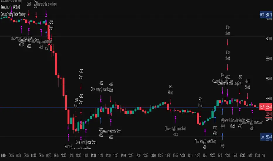
Market Matrix ViewThis technical indicator is designed to provide traders with a quick and integrated view of market dynamics by combining several popular indicators into a single tool. It's not a magic bullet, but a practical aid for analyzing buying/selling pressure, trends, volume, and divergences, saving you time in the decision-making process. Built for flexibility, the indicator adapts to various trading styles (scalping, swing, or long-term) and offers customizable settings to suit your needs.
🟡 Multi-Timeframe Trends
➤ This section displays the trend direction (bullish, bearish, or neutral) across 15-minute, 1-hour, 4-hour, and Daily timeframes, providing multi-timeframe market context. Timeframes lower than the one currently selected will show "N/A."
➤It utilizes fast and slow Exponential Moving Averages (EMAs) for each timeframe:
15m: Fast EMA 42, Slow EMA 170
1h: Fast EMA 40, Slow EMA 100
4h: Fast EMA 36, Slow EMA 107
Daily: Fast EMA 20, Slow EMA 60
🟡 Smart Flow & RVOL
➤ This section displays "Buying Pressure" or "Selling Pressure" signals based on indicator confluence, alongside volume activity ("High Activity," "Normal Activity," or "Low Activity").
➤ Smart Flow combines Chaikin Money Flow (CMF) and Money Flow Index (MFI) to detect buying/selling pressure. CMF measures money flow based on price position within the high-low range, while MFI analyzes money flow considering typical price and volume. A signal is generated only when both indicators simultaneously increase/decrease beyond an adjustable threshold ("Buy/Sell Sensitivity") and volume exceeds a Simple Moving Average (SMA) scaled by the "Volume Multiplier."
➤ RVOL (Relative Volume) calculates relative volume separately for bullish and bearish candles, comparing recent volume (fast SMA) with a reference volume (slow SMA). Thresholds are adjusted based on the selected mode.
🟡 ADX & RSI
This section displays trend strength ("Strong," "Moderate," or "Weak"), its direction ("Bullish" or "Bearish"), and the RSI momentum status ("Overbought," "Oversold," "Buy/Sell Momentum," or "Neutral").
➤ ADX (Average Directional Index) measures trend strength (above 40 = "Strong," 20–40 = "Moderate," below 20 = "Weak"). Direction is determined by comparing +DI (upward movement) with -DI (downward movement). Additionally, an arrow indicates whether the trend's strength is decreasing or increasing.
➤RSI (Relative Strength Index) evaluates price momentum. Extreme levels (above 80/85 = "Overbought," below 15/20 = "Oversold") and intermediate zones (47–53 = "Neutral," above 53 = "Buy Momentum," below 47 = "Sell Momentum") are adjusted based on the selected mode.
🟡 When these signals are active for a potential trade setup, the table's background lights up green or red, respectively.
🟡 Volume Spikes
➤This feature highlights bars with significantly higher volume than the recent average, coloring them yellow on the chart to draw attention to intense market activity.
➤It uses the Z-Score method to detect volume anomalies. Current volume is compared to a 10-bar Simple Moving Average (SMA) and the standard deviation of volume over the same period. If the Z-Score exceeds a certain threshold, the bar is marked as a volume spike.
🟡 Divergences (Volume Divergence Detection)
➤ This feature marks divergences between price and technical indicators on the chart, using diamond-shaped labels (green for bullish divergences, red for bearish divergences) to signal potential trend reversals.
➤ It compares price deviations from a Simple Moving Average (SMA) with deviations of three indicators: Chaikin Money Flow (CMF), Money Flow Index (MFI), and On-Balance Volume (OBV). A bullish divergence occurs when price falls below its average, but CMF, MFI, and OBV rise above their averages, indicating hidden accumulation. A bearish divergence occurs when price rises above its average, but CMF, MFI, and OBV fall, suggesting distribution. The length of the moving averages is adjustable (default 13/10/5 bars for Scalping/Balanced/Swing), and detection thresholds are scaled by "Divergence Sensitivity" (default 1.0).
🟡 Adaptive Stop-Loss (ATR)
➤Draws dynamic stop-loss lines (red, dashed) on the chart for buy or sell signals, helping traders manage risk.Uses the Average True Range (ATR) to calculate stop-loss levels, set at low/high ± ATR × multiplier
🟡 Alerts for trend direction changes in the Info Panel:
➤ Triggers notifications when the trend shifts to Bullish (when +DI crosses above -DI) or Bearish (when +DI crosses below -DI), helping you stay informed about key market shifts.
How to use: Set alerts in Trading View for “Trend Changed to Bullish” or “Trend Changed to Bearish” with “Once Per Bar Close” for reliable signals.
🟡 Settings (Inputs)
➤ The indicator offers customizable settings to fit your trading style, but it's already optimized for Scalping (1m–15m), Balanced (16m–3h59m), and Swing (4h–Daily) modes, which automatically adjust based on the selected timeframe. The visible inputs allow you to adjust the following parameters:
Show Info Panel: Enables/disables the information panel (default: enabled).
Show Volume Spikes: Turns on/off coloring for volume spike bars (default: enabled).
Spike Sensitivity: Controls the Z-Score threshold for detecting volume spikes (default: 2.0; lower values increase signal frequency).
Show Divergence: Enables/disables the display of divergence labels (default: enabled).
Divergence Sensitivity: Adjusts the thresholds for divergence detection (default: 1.0; higher values reduce sensitivity).
Divergence Lookback Length: Sets the length of the moving averages used for divergences (default: 5, automatically adjusted to 13/10/5 for Scalping/Balanced/Swing).
RVOL Reference Period: Defines the reference period for relative volume (default: 20, automatically adjusted to 7/15/20).
RSI Length: Sets the RSI length (default: 14, automatically adjusted to 5/10/14).
Buy Sensitivity: Controls the increase threshold for Buying Pressure signals (default: 0.007; higher values reduce frequency).
Sell Sensitivity: Controls the decrease threshold for Selling Pressure signals (default: 0.007; higher values reduce frequency).
Volume Multiplier (B/S Pressure): Adjusts the volume threshold for Smart Flow signals (default: 0.6; higher values require greater volume).
🟡 This indicator is created to simplify market analysis, but I am not a professional in Pine Script or technical indicators. This indicator is not a standalone solution. For optimal results, it must be integrated into a well-defined trading strategy that includes risk management and other confirmations.
Vix_Fix Enhanced MTF [Cometreon]The VIX Fix Enhanced is designed to detect market bottoms and spikes in volatility, helping traders anticipate major reversals with precision. Unlike standard VIX Fix tools, this version allows you to control the standard deviation logic, switch between chart styles, customize visual outputs, and set up advanced alerts — all with no repainting.
🧠 Logic and Calculation
This indicator is based on Larry Williams' VIX Fix and integrates features derived from community requests/advice, such as inverse VIX logic.
It calculates volatility spikes using a customizable standard deviation of the lows and compares it to a moving high to identify potential reversal points.
All moving average logic is based on Cometreon's proprietary library, ensuring accurate and optimized calculations on all 15 moving average types.
🔷 New Features and Improvements
🟩 Custom Visual Styles
Choose how you want your VIX data displayed:
Line
Step Line
Histogram
Area
Column
You can also flip the orientation (bottom-up or top-down), change the source ticker, and tailor the display to match your charting preferences.
🟩 Multi-MA Standard Deviation Calculation
Customize the standard deviation formula by selecting from 15 different moving averages:
SMA (Simple Moving Average)
EMA (Exponential Moving Average)
WMA (Weighted Moving Average)
RMA (Smoothed Moving Average)
HMA (Hull Moving Average)
JMA (Jurik Moving Average)
DEMA (Double Exponential Moving Average)
TEMA (Triple Exponential Moving Average)
LSMA (Least Squares Moving Average)
VWMA (Volume-Weighted Moving Average)
SMMA (Smoothed Moving Average)
KAMA (Kaufman’s Adaptive Moving Average)
ALMA (Arnaud Legoux Moving Average)
FRAMA (Fractal Adaptive Moving Average)
VIDYA (Variable Index Dynamic Average)
This gives you fine control over how volatility is measured and allows tuning the sensitivity for different market conditions.
🟩 Full Control Over Percentile and Deviation Conditions
You can enable or disable lines for standard deviation and percentile conditions, and define whether you want to trigger on over or under levels — adapting the indicator to your exact logic and style.
🟩 Chart Type Selection
You're no longer limited to candlestick charts! Now you can use Vix_Fix with different chart formats, including:
Candlestick
Heikin Ashi
Renko
Kagi
Line Break
Point & Figure
🟩 Multi-Timeframe Compatibility Without Repainting
Use a different timeframe from your chart with confidence. Signals remain stable and do not repaint. Perfect for spotting long-term reversal setups on lower timeframes.
🟩 Alert System Ready
Configure alerts directly from the indicator’s panel when conditions for over/under signals are met. Stay informed without needing to monitor the chart constantly.
🔷 Technical Details and Customizable Inputs
This indicator includes full control over the logic and appearance:
1️⃣ Length Deviation High - Adjusts the lookback period used to calculate the high deviation level of the VIX logic. Shorter values make it more reactive; longer values smooth out the signal.
2️⃣ Ticker - Choose a different chart type for the calculation, including Heikin Ashi, Renko, Kagi, Line Break, and Point & Figure.
3️⃣ Style VIX - Change the visual style (Line, Histogram, Column, etc.), adjust line width, and optionally invert the display (bottom-to-top).
📌 Fill zones for deviation and percentile are active only in Line and Step Line modes
4️⃣ Use Standard Deviation Up / Down - Enable the overbought and oversold zone logic based on upper and lower standard deviation bands.
5️⃣ Different Type MA (for StdDev) - Choose from 15 different moving averages to define the calculation method for standard deviation (SMA, EMA, HMA, JMA, etc.), with dedicated parameters like Phase, Sigma, and Offset for optimized responsiveness.
6️⃣ BB Length & Multiplier - Adjust the period and multiplier for the standard deviation bands, similar to how Bollinger Bands work.
7️⃣ Show StdDev Up / Down Line - Enable or disable the visibility of upper and lower standard deviation boundaries.
8️⃣ Use Percentile & Length High - Activate the percentile-based logic to detect extreme values in historical volatility using a customizable lookback length.
9️⃣ Highest % / Lowest % - Set the high and low percentile thresholds (e.g., 85 for high, 99 for low) that will be used to trigger over/under signals.
🔟 Show High / Low Percentile Line - Toggle the visual display of the percentile boundaries directly on the chart for clearer signal reference.
1️⃣1️⃣ Ticker Settings – Customize parameters for special chart types such as Renko, Heikin Ashi, Kagi, Line Break, and Point & Figure, adjusting reversal, number of lines, ATR length, etc.
1️⃣2️⃣ Timeframe – Enables using SuperTrend on a higher timeframe.
1️⃣3️⃣ Wait for Timeframe Closes -
✅ Enabled – Displays Vix_Fix smoothly with interruptions.
❌ Disabled – Displays Vix_Fix smoothly without interruptions.
☄️ If you find this indicator useful, leave a Boost to support its development!
Every feedback helps to continuously improve the tool, offering an even more effective trading experience. Share your thoughts in the comments! 🚀🔥

15Min Opening Range & Midline (UTC+2) This TradingView script draws the 15-minute Opening Range of the day based on a user-defined start time and plots the high, low, and midline of this range. It works by capturing the high and low of the first 15 minutes of the session, and then extending them for the rest of the trading day. The midline is calculated as the average of the high and low values.
Key Features:
User-configurable start time: Define the hour and minute for when the opening range should start based on your local time zone.
Line customization: Choose the color and line style (solid, dashed, dotted) for the high, low, and midline.
Easy-to-read visual representation: The high and low lines extend across the chart from the range start, with the midline placed in the center.
Dynamic updates: The indicator resets at the start of each new trading day and updates the opening range lines accordingly.
Perfect for:
Traders looking to monitor the initial market range during the first 15 minutes of trading.
Identifying key support and resistance levels based on early price action.
Providing a midline to assess market bias and potential breakouts.
Notes:
The indicator calculates everything based on the local time zone you define and automatically adjusts to your desired start time.
It will not redraw lines; once drawn, they remain on the chart until the next session.
Schmit Trading LiquidityDescription
Schmit Trading Liquidity Marker automatically spots and labels open liquidity sweep levels by detecting classic stop-run patterns (Bull→Bear for highs, Bear→Bull for lows) across multiple timeframes. Lines are drawn exactly at the wick of the triggering candle and removed as soon as price “sweeps” through them, keeping your chart clean and focused on live levels only.
How It Works
1. Pattern Detection
• Liquidity High: When a bullish candle is immediately followed by a bearish candle (Bull→Bear), the script records the higher of the two wicks.
• Liquidity Low: When a bearish candle is immediately followed by a bullish candle (Bear→Bull), the script records the lower of the two wicks.
2. Multi-Timeframe Support
• Choose up to six timeframes (5 min, 15 min, 30 min, 1 h, 4 h, daily) via checkboxes.
• Each timeframe is evaluated independently, and liquidity levels are drawn on your current chart.
3. Precision Wick Placement
• Lines start at bar_index – 1 so they align exactly with the wick of the signal candle, regardless of your chart’s timeframe.
4. Automatic Cleanup
• As soon as price closes beyond a drawn line (sweep), that line is deleted automatically.
Inputs
Input Name Description
Show 5 min. Enable liquidity detection on the 5-minute timeframe.
Show 15 min. Enable liquidity detection on the 15-minute timeframe.
Show 30 min. Enable liquidity detection on the 30-minute timeframe.
Show 1 h. Enable liquidity detection on the 1-hour timeframe.
Show 4 h. Enable liquidity detection on the 4-hour timeframe.
Show 1 D. Enable liquidity detection on the daily timeframe.
High Line Color. Color of Bull→Bear (liquidity high) lines (default: red).
Low Line Color. Color of Bear→Bull (liquidity low) lines (default: blue).
Line Length. How many bars each liquidity line extends to the right.
Usage Tips
• Focus on Live Zones: Combine with volume or order-flow tools to confirm genuine
liquidity sweeps.
• Multiple TFs: Enable higher timeframes for major liquidity clusters; lower timeframes
for fine‐tuning entries.
• Chart Cleanliness: Lines self‐delete on sweep, ensuring no manual cleanup is needed.
⸻
Disclosure & License
This indicator is Open-Source under the Mozilla Public License 2.0. Feel free to review, adapt, and improve the code. No performance guarantees—use responsibly and backtest any strategy before trading live.
