Uptrick: Volatility Weighted CloudIntroduction
The Volatility Weighted Cloud (VWC) is a trend-tracking overlay that combines adaptive volatility-based bands with a multi-source smoothed price cloud to visualize market bias. It provides users with a dynamic structure that adapts to volatility conditions while maintaining a persistent visual record of trend direction. By incorporating configurable smoothing techniques, percentile-ranked volatility, and multi-line cloud construction, the indicator allows traders to interpret price context more effectively without relying on raw price movement alone.
Overview
The script builds a smoothed price basis using the open, and close prices independently, and uses these to construct a layered visual cloud. This cloud serves both as a reference for price structure and a potential area of dynamic support and resistance. Alongside this cloud, adaptive upper and lower bands are plotted using volatility that scales with percentile rank. When price closes above or below these bands, the script interprets that as a breakout and updates the trend bias accordingly.
Candle coloring is persistent and reflects the most recent confirmed signal. Labels can optionally be placed on the chart when the trend bias flips, giving traders additional visual reference points. The indicator is designed to be both flexible and visually compact, supporting different strategies and timeframes through its detailed configuration options.
Originality
This script introduces originality through its combined use of percentile-ranked volatility, adaptive envelope sizing, and multi-source cloud construction. Unlike static-band indicators, the Volatility Weighted Cloud adjusts its band width based on where current volatility ranks within a defined lookback range. This dynamic scaling allows for smoother signal behavior during low-volatility environments and more responsive behavior during high-volatility phases.
Additionally, instead of using a single basis line, the indicator computes two separate smoothed lines for open and close. These are rendered into a shaded visual cloud that reflects price structure more completely than traditional moving average overlays. The use of ALMA and MAD, both less commonly applied in volatility-band overlays, adds further control over smoothing behavior and volatility measurement, enhancing its adaptability across different market types.
Inputs
Group: Core
Basis Length (short-term): The number of bars used for calculating the primary basis line. Affects how quickly the basis responds to price changes.
Basis Type: Option to choose between EMA and ALMA. EMA provides a standard exponential average; ALMA offers a centered, Gaussian-weighted average with reduced lag.
ALMA Offset: Determines the balance point of the ALMA window. Only applies when ALMA is selected.
Sigma: Sets the width of the ALMA smoothing window, influencing how much smoothing is applied.
Basis Smoothing EMA: Adds additional EMA-based smoothing to the computed basis line for noise reduction.
Group: Volatility & Bands
Volatility: Choose between StDev (standard deviation) and MAD (median absolute deviation) for measuring price volatility.
Vol Length (short-term): Length of the window used for calculating volatility.
Vol Smoothing EMA: Smooths the raw volatility value to stabilize band behavior.
Min Multiplier: Minimum multiplier applied to volatility when forming the adaptive bands.
Max Multiplier: Maximum multiplier applied at high volatility percentile.
Volatility Rank Lookback: Number of bars used to calculate the percentile rank of current volatility.
Show Adaptive Bands: Enables or disables the display of upper and lower volatility bands on the chart.
Group: Trend Switch Labels
Show Trend Switch Labels: Toggles the appearance of labels when the trend direction changes.
Label Anchor: Defines whether the labels are anchored to recent highs/lows or to the main basis line.
ATR Length (offset): Length used for calculating ATR, which determines label offset distance.
ATR Offset (multiplier): Multiplies the ATR value to place labels away from price bars for better visibility.
Label Size: Allows selection of label size (tiny to huge) to suit different chart setups.
Features
Adaptive Volatility Bands: The indicator calculates volatility using either standard deviation or MAD. It then applies an EMA smoothing layer and scales the band width dynamically based on the percentile rank of volatility over a user-defined lookback window. This avoids fixed-width bands and allows the indicator to adapt to changing volatility regimes in real time.
Volatility Method Options: Users can switch between two volatility measurement methods:
➤ Standard Deviation (StDev): Captures overall price dispersion, but may be sensitive to spikes.
➤ Median Absolute Deviation (MAD): A more robust measure that reduces the effect of outliers, making the bands less jumpy during erratic price behavior.
Basis Type Options: The core price basis used for cloud and bands can be built from:
➤ Exponential Moving Average (EMA): Fast-reacting and widely used in trend systems.
➤ Arnaud Legoux Moving Average (ALMA): A smoother, more centered alternative that offers greater control through offset and sigma parameters.
Multi-Line Basis Cloud: The cloud is formed by plotting two individually smoothed basis lines from open and close prices. A filled area is created between the open and close basis lines. This cloud serves as a dynamic support or resistance zone, allowing users to identify possible reversal areas. Price moving through or rejecting from the cloud can be interpreted contextually, especially when combined with band-based signals.
Persistent Trend Bias Coloring: The indicator uses the last confirmed breakout (above upper band or below lower band) to determine bias. This bias is reflected in the color of every subsequent candle, offering a persistent visual cue until a new signal is triggered. It helps simplify trend recognition, especially in choppy or sideways markets.
Trend Switch Labels: When enabled, the script places labeled markers at the exact bar where the bias direction switches. Labels are anchored either to recent highs/lows or to the main basis line, and spaced vertically using an ATR-based offset. This allows the trader to quickly locate historical trend transitions.
Alert Conditions: Two built-in alert conditions are available:
➤ Long Signal: Triggered when the close crosses above the upper adaptive band.
➤ Short Signal: Triggered when the close crosses below the lower adaptive band.
These conditions can be used for custom alerts, automation, or external signaling tools.
Display Control and Flexibility: Users can disable the adaptive bands for a cleaner layout while keeping the basis cloud and candle coloring active. The indicator can be tuned for fast or slow response depending on the strategy in use, and is suitable for intraday, swing, or position trading.
Summary
The Volatility Weighted Cloud is a configurable trend-following overlay that uses adaptive volatility bands and a structured cloud system to help visualize market bias. By combining EMA or ALMA smoothing with percentile-ranked volatility and a four-line price structure, it provides a flexible and informative charting layer. Its key strengths lie in the use of dynamic envelopes, visually persistent trend indication, and clearly defined breakout zones that adapt to current volatility conditions.
Disclaimer
This indicator is for informational and educational purposes only. Trading involves risk and may not be suitable for all investors. Past performance does not guarantee future results.
"Exponential"に関するスクリプトを検索

AMHA + 4 EMAs + EMA50/200 Counter + Avg10CrossesDescription:
This script combines two types of Heikin-Ashi visualization with multiple Exponential Moving Averages (EMAs) and a counting function for EMA50/200 crossovers. The goal is to make trends more visible, measure recurring market cycles, and provide statistical context without generating trading signals.
Logic in Detail:
Adaptive Median Heikin-Ashi (AMHA):
Instead of the classic Heikin-Ashi calculation, this method uses the median of Open, High, Low, and Close. The result smooths out price movements, emphasizes trend direction, and reduces market noise.
Standard Heikin-Ashi Overlay:
Classic HA candles are also drawn in the background for comparison and transparency. Both HA types can be shifted below the chart’s price action using a customizable Offset (Ticks) parameter.
EMA Structure:
Five exponential moving averages (21, 50, 100, 200, 500) are included to highlight different trend horizons. EMA50 and EMA200 are emphasized, as their crossovers are widely monitored as potential trend signals. EMA21 and EMA100 serve as additional structure layers, while EMA500 represents the long-term trend.
EMA50/200 Counter:
The script counts how many bars have passed since the last EMA50/200 crossover. This makes it easy to see the age of the current trend phase. A colored label above the chart displays the current counter.
Average of the Last 10 Crossovers (Avg10Crosses):
The script stores the last 10 completed count phases and calculates their average length. This provides historical context and allows traders to compare the current cycle against typical past behavior.
Benefits for Analysis:
Clearer trend visualization through adaptive Heikin-Ashi calculation.
Multi-EMA setup for quick structural assessment.
Objective measurement of trend phase duration.
Statistical insight from the average cycle length of past EMA50/200 crosses.
Flexible visualization through adjustable offset positioning below the price chart.
Usage:
Add the indicator to your chart.
For a clean look, you may switch your chart type to “Line” or hide standard candlesticks.
Interpret visual signals:
White candles = bullish phases
Orange candles = bearish phases
EMAs = structural trend filters (e.g., EMA200 as a long-term boundary)
The counter label shows the current number of bars since the last cross, while Avg10 represents the historical mean.
Special Feature:
This script is not a trading system. It does not provide buy/sell recommendations. Instead, it serves as a visual and statistical tool for market structure analysis. The unique combination of Adaptive Median Heikin-Ashi, multi-EMA framework, and EMA50/200 crossover statistics makes it especially useful for trend-followers and swing traders who want to add cycle-length analysis to their toolkit.
Anchored EMA/VWAP### Anchored EMA/VWAP Indicator
**Description:**
The **Anchored EMA/VWAP Indicator** is a powerful and versatile tool designed for traders seeking to analyze price trends and momentum from a user-defined anchor point in time. Built for TradingView using Pine Script v6, this indicator calculates and displays multiple **Exponential Moving Averages (EMAs)**, **Volume-Weighted Exponential Moving Averages (VWEMAs)**, and a **Volume-Weighted Average Price (VWAP)**, all anchored to a specific date and time chosen by the user. By anchoring these calculations, traders can focus on price action relative to significant market events, such as news releases, earnings reports, or key support/resistance levels.
The indicator supports multi-timeframe (MTF) analysis, allowing users to compute EMAs, VWEMAs, and VWAP on a higher or custom timeframe (e.g., 5-minute, 1-hour, daily) while overlaying the results on the current chart. It also includes customizable cross signals for EMA and VWEMA pairs, marked with distinct shapes (circles, diamonds, squares) to highlight potential trend changes or reversals. These features make the indicator ideal for trend-following, momentum trading, and identifying key price levels across various markets, including stocks, forex, cryptocurrencies, and commodities.
**Key Features:**
- **Anchored Calculations**: EMAs, VWEMAs, and VWAP start calculations from a user-specified anchor time, enabling analysis relative to significant market moments.
- **Multi-Timeframe Support**: Compute indicators on any timeframe (e.g., 60-minute, daily) and display them on the chart’s timeframe for flexible analysis.
- **Customizable EMAs and VWEMAs**: Four EMAs and four VWEMAs with adjustable lengths (default: 9, 21, 50, 100) and colors, with options to show or hide each.
- **Volume-Weighted Metrics**: VWAP and VWEMAs incorporate volume data, providing a more robust representation of market activity compared to standard EMAs.
- **Cross Signals**: Visual markers (circles, diamonds, squares) for crossovers between EMA and VWEMA pairs, with customizable visibility to highlight bullish (up) or bearish (down) signals.
- **User-Friendly Interface**: Organized input groups for General, EMA, VWEMA, VWAP, Arrow Settings, and Cross Visibility, with intuitive inline inputs for length and color customization.
- **Visual Clarity**: Overlaid on the price chart with distinct colors and line styles (dotted for EMAs, dashed for VWEMAs, solid for VWAP) to ensure easy interpretation.
**How to Use:**
1. **Set the Anchor Time**: Click a specific bar or enter a date/time (default: June 1, 2025) to start calculations from a significant market event.
2. **Select Timeframe**: Choose a timeframe (e.g., "5" for 5-minute, "D" for daily) to compute the indicators, allowing alignment with your trading strategy.
3. **Customize EMAs and VWEMAs**: Adjust lengths and colors for up to four EMAs and VWEMAs, and toggle their visibility to focus on relevant lines.
4. **Enable VWAP**: Display the anchored VWAP to identify volume-weighted price levels, useful as dynamic support/resistance.
5. **Monitor Cross Signals**: Enable cross visibility for specific EMA or VWEMA pairs to spot potential trend changes. Bullish crosses (e.g., shorter EMA crossing above longer EMA) are marked with green shapes below the bar, while bearish crosses are marked with red shapes above the bar.
6. **Interpret Signals**: Use EMA/VWEMA crossovers for trend confirmation, VWAP as a mean-reversion level, and volume-weighted VWEMAs for momentum analysis in high-volume markets.
**Use Cases:**
- **Trend Trading**: Identify trend direction using EMA and VWEMA crossovers, with shorter lengths (e.g., 9, 21) for faster signals and longer lengths (e.g., 50, 100) for trend confirmation.
- **Mean Reversion**: Use the anchored VWAP as a dynamic support/resistance level to trade pullbacks or breakouts.
- **Event-Based Analysis**: Anchor the indicator to significant events (e.g., earnings, economic data releases) to analyze price behavior post-event.
- **Multi-Timeframe Strategies**: Combine higher timeframe EMAs/VWAPs with lower timeframe price action for high-probability setups.
**Settings:**
- **Anchor Time**: Set the starting point for calculations (default: June 1, 2025).
- **Timeframe**: Choose the timeframe for calculations (default: 5-minute).
- **EMA/VWEMA Lengths**: Default lengths of 9, 21, 50, and 100 for both EMAs and VWEMAs, adjustable per user preference.
- **Colors**: Customizable colors with slight transparency for visual clarity.
- **Cross Visibility**: Toggle specific EMA and VWEMA cross signals (e.g., EMA1/EMA2, VWEMA1/VWEMA3) to reduce chart clutter.
- **Arrow Colors**: Green for bullish crosses, red for bearish crosses.
**Notes:**
- The indicator is overlaid on the price chart, ensuring seamless integration with price action analysis.
- VWEMAs and VWAP are volume-sensitive, making them particularly effective in markets with significant volume fluctuations.
- Ensure the anchor time is set to a valid historical or future bar to avoid calculation errors.
- Cross signals are conditional on non-NA values to prevent false positives during initialization.
**Author**: NEPOLIX
**Version**: 6 (Pine Script v6)
**Published**: For TradingView Community
This indicator is a must-have for traders looking to combine anchored, volume-weighted, and multi-timeframe analysis into a single, customizable tool. Whether you're a day trader, swing trader, or long-term investor, the Anchored EMA/VWAP Indicator provides actionable insights for informed trading decisions.

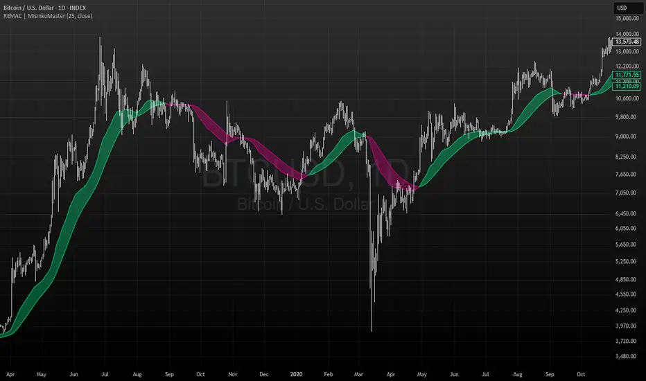
RMA EMA Crossover | MisinkoMasterThe RMA EMA Crossover (REMAC) is a trend-following overlay indicator designed to detect shifts in market momentum using the interaction between a smoothed RMA (Relative Moving Average) and its EMA (Exponential Moving Average) counterpart.
This combination provides fast, adaptive signals while reducing noise, making it suitable for a wide range of markets and timeframes.
🔎 Methodology
RMA Calculation
The Relative Moving Average (RMA) is calculated over the user-defined length.
RMA is a type of smoothed moving average that reacts more gradually than a standard EMA, providing a stable baseline.
EMA of RMA
An Exponential Moving Average (EMA) is then applied to the RMA, creating a dual-layer moving average system.
This combination amplifies trend signals while reducing false crossovers.
Trend Detection (Crossover Logic)
Bullish Signal (Trend Up) → When RMA crosses above EMA.
Bearish Signal (Trend Down) → When EMA crosses above RMA.
This simple crossover system identifies the direction of momentum shifts efficiently.
📈 Visualization
RMA and EMA are plotted directly on the chart.
Colors adapt dynamically to the current trend:
Cyan / Green hues → RMA above EMA (bullish momentum).
Magenta / Red hues → EMA above RMA (bearish momentum).
Filled areas between the two lines highlight zones of trend alignment or divergence, making it easier to spot reversals at a glance.
⚡ Features
Adjustable length parameter for RMA and EMA.
Overlay format allows for direct integration with price charts.
Visual trend scoring via color and fill for rapid assessment.
Works well across all asset classes: crypto, forex, stocks, indices.
✅ Use Cases
Trend Following → Stay on the right side of the market by following momentum shifts.
Reversal Detection → Crossovers highlight early trend changes.
Filter for Trading Systems → Use as a confirmation overlay for other indicators or strategies.
Visual Market Insight → Filled zones provide immediate context for trend strength.
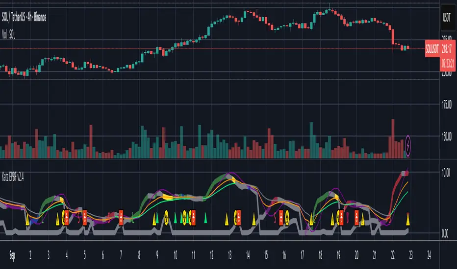
Katz Exploding PowerBand FilterUnderstanding the Katz Exploding PowerBand Filter (EPBF) v2.4
1. Indicator Overview
The Katz Exploding PowerBand Filter (EPBF) is an advanced technical indicator designed to identify moments of expanding bullish or bearish momentum, often referred to as "power." It operates as a standalone oscillator in a separate pane below the main price chart.
Its primary goal is to measure underlying market strength by calculating custom "Bull" and "Bear" power components. These components are then filtered through a versatile moving average and a dual signal line system to generate clear entry and exit signals. This indicator is not a simple momentum oscillator; it uses a unique calculation based on exponential envelopes of both price and squared price to derive its values.
2. On-Chart Lines and Components
The indicator pane consists of five main lines:
Bullish Component (Thick Green/Blue/Yellow/Gray Line): This is the core of the indicator. It represents the calculated bullish "power" or momentum in the market.
Bright Green: Indicates a strong, active long signal condition.
Blue: Shows the bull component is above the MA filter, but the filter itself is still pointing down—a potential sign of a reversal or weakening downtrend.
Yellow: A warning sign that bullish power is weakening and has fallen below the primary signal lines.
Gray: Represents neutral or insignificant bullish power.
Bearish Component (Thick Red/Purple/Yellow/Gray Line): This line represents the calculated bearish "power" or downward momentum.
Bright Red: Indicates a strong, active short signal condition.
Purple: Shows the bear component is above the MA filter, but the filter itself is still pointing down—a sign of potential trend continuation.
Yellow: A warning sign that bearish power is weakening.
Gray: Represents neutral or insignificant bearish power.
MA Filter (Purple Line): This is the main filter, calculated using the moving average type and length you select in the settings (e.g., HullMA, EMA). The Bull and Bear components are compared against this line to determine the underlying trend bias.
Signal Line 1 (Orange Line): A fast Exponential Moving Average (EMA) of the stronger power component. It acts as the first level of dynamic support or resistance for the power lines.
Signal Line 2 (Lime/Gray Line): A slower EMA that acts as a confirmation filter.
Lime Green: The line turns lime when it is rising and the faster Signal Line 1 is above it, indicating a confirmed bullish trend in momentum.
Gray: Indicates a neutral or bearish momentum trend.
3. On-Chart Symbols and Their Meanings
Various characters are plotted at the bottom of the indicator pane to provide clear, actionable signals.
L (Pre-Long Signal): The first sign of a potential long entry. It appears when the Bullish Component rises and crosses above both signal lines for the first time.
S (Pre-Short Signal): The first sign of a potential short entry. It appears when the Bearish Component rises and crosses above both signal lines for the first time.
▲ (Post-Long Signal): A stronger confirmation for a long entry. It appears with the 'L' signal only if the momentum trend is also confirmed bullish (i.e., the slower Signal Line 2 is lime green).
▼ (Post-Short Signal): A stronger confirmation for a short entry. It appears with the 'S' signal only if the momentum trend is confirmed bullish.
Exit / Take-Profit Symbols:
These symbols appear when a power component crosses below a line, suggesting that momentum is fading and it may be time to take profit.
⚠️ (Exit Signal 1): The Bull/Bear component has crossed below the main MA Filter. This is the first and most sensitive take-profit signal.
☣️ (Exit Signal 2): The Bull/Bear component has crossed below the faster Signal Line 1. This is a moderate take-profit signal.
🚼 (Exit Signal 3): The Bull/Bear component has crossed below the slower Signal Line 2. This is the slowest take-profit signal, suggesting the trend is more definitively exhausted.
4. Trading Strategy and Rules
Long Entry Rules:
Initial Signal: Wait for an L to appear at the bottom of the indicator. This confirms that bullish power is expanding.
Confirmation (Recommended): For a higher-probability trade, wait for a green ▲ symbol to appear. This confirms the underlying momentum trend aligns with the signal.
Entry: Enter a long (buy) position on the opening of the next candle after the signal appears.
Short Entry Rules:
Initial Signal: Wait for an S to appear at the bottom of the indicator. This confirms that bearish power is expanding.
Confirmation (Recommended): For a higher-probability trade, wait for a maroon ▼ symbol to appear. This confirms the underlying momentum trend aligns with the signal.
Entry: Enter a short (sell) position on the opening of the next candle after the signal appears.
Take Profit (TP) Rules:
The indicator provides three levels of take-profit signals. You can choose to exit your entire position or scale out at each level.
For a long trade, exit when you see ⚠️, ☣️, or 🚼 appear below the Bullish Component.
For a short trade, exit when you see ⚠️, ☣️, or 🚼 appear below the Bearish Component.
Stop Loss (SL) Rules:
The indicator does not provide an explicit stop loss. You must use your own risk management rules. Common methods include:
Swing High/Low: For a long position, place your stop loss below the most recent significant swing low on the price chart. For a short position, place it above the most recent swing high.
ATR-Based: Use an Average True Range (ATR) indicator to set a volatility-based stop loss.
Fixed Percentage: Risk a fixed percentage (e.g., 1-2%) of your account on the trade.
5. Disclaimer
This indicator is a tool for technical analysis and should not be considered financial advice. All trading involves significant risk, and past performance is not indicative of future results. The signals generated by this indicator are probabilistic and can result in losing trades. Always use proper risk management, such as setting a stop loss, and never risk more than you are willing to lose. It is recommended to backtest this indicator and use it in conjunction with other forms of analysis before trading with real capital. The indicator should only be used for educational purposes.
Small Business Economic Conditions - Statistical Analysis ModelThe Small Business Economic Conditions Statistical Analysis Model (SBO-SAM) represents an econometric approach to measuring and analyzing the economic health of small business enterprises through multi-dimensional factor analysis and statistical methodologies. This indicator synthesizes eight fundamental economic components into a composite index that provides real-time assessment of small business operating conditions with statistical rigor. The model employs Z-score standardization, variance-weighted aggregation, higher-order moment analysis, and regime-switching detection to deliver comprehensive insights into small business economic conditions with statistical confidence intervals and multi-language accessibility.
1. Introduction and Theoretical Foundation
The development of quantitative models for assessing small business economic conditions has gained significant importance in contemporary financial analysis, particularly given the critical role small enterprises play in economic development and employment generation. Small businesses, typically defined as enterprises with fewer than 500 employees according to the U.S. Small Business Administration, constitute approximately 99.9% of all businesses in the United States and employ nearly half of the private workforce (U.S. Small Business Administration, 2024).
The theoretical framework underlying the SBO-SAM model draws extensively from established academic research in small business economics and quantitative finance. The foundational understanding of key drivers affecting small business performance builds upon the seminal work of Dunkelberg and Wade (2023) in their analysis of small business economic trends through the National Federation of Independent Business (NFIB) Small Business Economic Trends survey. Their research established the critical importance of optimism, hiring plans, capital expenditure intentions, and credit availability as primary determinants of small business performance.
The model incorporates insights from Federal Reserve Board research, particularly the Senior Loan Officer Opinion Survey (Federal Reserve Board, 2024), which demonstrates the critical importance of credit market conditions in small business operations. This research consistently shows that small businesses face disproportionate challenges during periods of credit tightening, as they typically lack access to capital markets and rely heavily on bank financing.
The statistical methodology employed in this model follows the econometric principles established by Hamilton (1989) in his work on regime-switching models and time series analysis. Hamilton's framework provides the theoretical foundation for identifying different economic regimes and understanding how economic relationships may vary across different market conditions. The variance-weighted aggregation technique draws from modern portfolio theory as developed by Markowitz (1952) and later refined by Sharpe (1964), applying these concepts to economic indicator construction rather than traditional asset allocation.
Additional theoretical support comes from the work of Engle and Granger (1987) on cointegration analysis, which provides the statistical framework for combining multiple time series while maintaining long-term equilibrium relationships. The model also incorporates insights from behavioral economics research by Kahneman and Tversky (1979) on prospect theory, recognizing that small business decision-making may exhibit systematic biases that affect economic outcomes.
2. Model Architecture and Component Structure
The SBO-SAM model employs eight orthogonalized economic factors that collectively capture the multifaceted nature of small business operating conditions. Each component is normalized using Z-score standardization with a rolling 252-day window, representing approximately one business year of trading data. This approach ensures statistical consistency across different market regimes and economic cycles, following the methodology established by Tsay (2010) in his treatment of financial time series analysis.
2.1 Small Cap Relative Performance Component
The first component measures the performance of the Russell 2000 index relative to the S&P 500, capturing the market-based assessment of small business equity valuations. This component reflects investor sentiment toward smaller enterprises and provides a forward-looking perspective on small business prospects. The theoretical justification for this component stems from the efficient market hypothesis as formulated by Fama (1970), which suggests that stock prices incorporate all available information about future prospects.
The calculation employs a 20-day rate of change with exponential smoothing to reduce noise while preserving signal integrity. The mathematical formulation is:
Small_Cap_Performance = (Russell_2000_t / S&P_500_t) / (Russell_2000_{t-20} / S&P_500_{t-20}) - 1
This relative performance measure eliminates market-wide effects and isolates the specific performance differential between small and large capitalization stocks, providing a pure measure of small business market sentiment.
2.2 Credit Market Conditions Component
Credit Market Conditions constitute the second component, incorporating commercial lending volumes and credit spread dynamics. This factor recognizes that small businesses are particularly sensitive to credit availability and borrowing costs, as established in numerous Federal Reserve studies (Bernanke and Gertler, 1995). Small businesses typically face higher borrowing costs and more stringent lending standards compared to larger enterprises, making credit conditions a critical determinant of their operating environment.
The model calculates credit spreads using high-yield bond ETFs relative to Treasury securities, providing a market-based measure of credit risk premiums that directly affect small business borrowing costs. The component also incorporates commercial and industrial loan growth data from the Federal Reserve's H.8 statistical release, which provides direct evidence of lending activity to businesses.
The mathematical specification combines these elements as:
Credit_Conditions = α₁ × (HYG_t / TLT_t) + α₂ × C&I_Loan_Growth_t
where HYG represents high-yield corporate bond ETF prices, TLT represents long-term Treasury ETF prices, and C&I_Loan_Growth represents the rate of change in commercial and industrial loans outstanding.
2.3 Labor Market Dynamics Component
The Labor Market Dynamics component captures employment cost pressures and labor availability metrics through the relationship between job openings and unemployment claims. This factor acknowledges that labor market tightness significantly impacts small business operations, as these enterprises typically have less flexibility in wage negotiations and face greater challenges in attracting and retaining talent during periods of low unemployment.
The theoretical foundation for this component draws from search and matching theory as developed by Mortensen and Pissarides (1994), which explains how labor market frictions affect employment dynamics. Small businesses often face higher search costs and longer hiring processes, making them particularly sensitive to labor market conditions.
The component is calculated as:
Labor_Tightness = Job_Openings_t / (Unemployment_Claims_t × 52)
This ratio provides a measure of labor market tightness, with higher values indicating greater difficulty in finding workers and potential wage pressures.
2.4 Consumer Demand Strength Component
Consumer Demand Strength represents the fourth component, combining consumer sentiment data with retail sales growth rates. Small businesses are disproportionately affected by consumer spending patterns, making this component crucial for assessing their operating environment. The theoretical justification comes from the permanent income hypothesis developed by Friedman (1957), which explains how consumer spending responds to both current conditions and future expectations.
The model weights consumer confidence and actual spending data to provide both forward-looking sentiment and contemporaneous demand indicators. The specification is:
Demand_Strength = β₁ × Consumer_Sentiment_t + β₂ × Retail_Sales_Growth_t
where β₁ and β₂ are determined through principal component analysis to maximize the explanatory power of the combined measure.
2.5 Input Cost Pressures Component
Input Cost Pressures form the fifth component, utilizing producer price index data to capture inflationary pressures on small business operations. This component is inversely weighted, recognizing that rising input costs negatively impact small business profitability and operating conditions. Small businesses typically have limited pricing power and face challenges in passing through cost increases to customers, making them particularly vulnerable to input cost inflation.
The theoretical foundation draws from cost-push inflation theory as described by Gordon (1988), which explains how supply-side price pressures affect business operations. The model employs a 90-day rate of change to capture medium-term cost trends while filtering out short-term volatility:
Cost_Pressure = -1 × (PPI_t / PPI_{t-90} - 1)
The negative weighting reflects the inverse relationship between input costs and business conditions.
2.6 Monetary Policy Impact Component
Monetary Policy Impact represents the sixth component, incorporating federal funds rates and yield curve dynamics. Small businesses are particularly sensitive to interest rate changes due to their higher reliance on variable-rate financing and limited access to capital markets. The theoretical foundation comes from monetary transmission mechanism theory as developed by Bernanke and Blinder (1992), which explains how monetary policy affects different segments of the economy.
The model calculates the absolute deviation of federal funds rates from a neutral 2% level, recognizing that both extremely low and high rates can create operational challenges for small enterprises. The yield curve component captures the shape of the term structure, which affects both borrowing costs and economic expectations:
Monetary_Impact = γ₁ × |Fed_Funds_Rate_t - 2.0| + γ₂ × (10Y_Yield_t - 2Y_Yield_t)
2.7 Currency Valuation Effects Component
Currency Valuation Effects constitute the seventh component, measuring the impact of US Dollar strength on small business competitiveness. A stronger dollar can benefit businesses with significant import components while disadvantaging exporters. The model employs Dollar Index volatility as a proxy for currency-related uncertainty that affects small business planning and operations.
The theoretical foundation draws from international trade theory and the work of Krugman (1987) on exchange rate effects on different business segments. Small businesses often lack hedging capabilities, making them more vulnerable to currency fluctuations:
Currency_Impact = -1 × DXY_Volatility_t
2.8 Regional Banking Health Component
The eighth and final component, Regional Banking Health, assesses the relative performance of regional banks compared to large financial institutions. Regional banks traditionally serve as primary lenders to small businesses, making their health a critical factor in small business credit availability and overall operating conditions.
This component draws from the literature on relationship banking as developed by Boot (2000), which demonstrates the importance of bank-borrower relationships, particularly for small enterprises. The calculation compares regional bank performance to large financial institutions:
Banking_Health = (Regional_Banks_Index_t / Large_Banks_Index_t) - 1
3. Statistical Methodology and Advanced Analytics
The model employs statistical techniques to ensure robustness and reliability. Z-score normalization is applied to each component using rolling 252-day windows, providing standardized measures that remain consistent across different time periods and market conditions. This approach follows the methodology established by Engle and Granger (1987) in their cointegration analysis framework.
3.1 Variance-Weighted Aggregation
The composite index calculation utilizes variance-weighted aggregation, where component weights are determined by the inverse of their historical variance. This approach, derived from modern portfolio theory, ensures that more stable components receive higher weights while reducing the impact of highly volatile factors. The mathematical formulation follows the principle that optimal weights are inversely proportional to variance, maximizing the signal-to-noise ratio of the composite indicator.
The weight for component i is calculated as:
w_i = (1/σᵢ²) / Σⱼ(1/σⱼ²)
where σᵢ² represents the variance of component i over the lookback period.
3.2 Higher-Order Moment Analysis
Higher-order moment analysis extends beyond traditional mean and variance calculations to include skewness and kurtosis measurements. Skewness provides insight into the asymmetry of the sentiment distribution, while kurtosis measures the tail behavior and potential for extreme events. These metrics offer valuable information about the underlying distribution characteristics and potential regime changes.
Skewness is calculated as:
Skewness = E / σ³
Kurtosis is calculated as:
Kurtosis = E / σ⁴ - 3
where μ represents the mean and σ represents the standard deviation of the distribution.
3.3 Regime-Switching Detection
The model incorporates regime-switching detection capabilities based on the Hamilton (1989) framework. This allows for identification of different economic regimes characterized by distinct statistical properties. The regime classification employs percentile-based thresholds:
- Regime 3 (Very High): Percentile rank > 80
- Regime 2 (High): Percentile rank 60-80
- Regime 1 (Moderate High): Percentile rank 50-60
- Regime 0 (Neutral): Percentile rank 40-50
- Regime -1 (Moderate Low): Percentile rank 30-40
- Regime -2 (Low): Percentile rank 20-30
- Regime -3 (Very Low): Percentile rank < 20
3.4 Information Theory Applications
The model incorporates information theory concepts, specifically Shannon entropy measurement, to assess the information content of the sentiment distribution. Shannon entropy, as developed by Shannon (1948), provides a measure of the uncertainty or information content in a probability distribution:
H(X) = -Σᵢ p(xᵢ) log₂ p(xᵢ)
Higher entropy values indicate greater unpredictability and information content in the sentiment series.
3.5 Long-Term Memory Analysis
The Hurst exponent calculation provides insight into the long-term memory characteristics of the sentiment series. Originally developed by Hurst (1951) for analyzing Nile River flow patterns, this measure has found extensive application in financial time series analysis. The Hurst exponent H is calculated using the rescaled range statistic:
H = log(R/S) / log(T)
where R/S represents the rescaled range and T represents the time period. Values of H > 0.5 indicate long-term positive autocorrelation (persistence), while H < 0.5 indicates mean-reverting behavior.
3.6 Structural Break Detection
The model employs Chow test approximation for structural break detection, based on the methodology developed by Chow (1960). This technique identifies potential structural changes in the underlying relationships by comparing the stability of regression parameters across different time periods:
Chow_Statistic = (RSS_restricted - RSS_unrestricted) / RSS_unrestricted × (n-2k)/k
where RSS represents residual sum of squares, n represents sample size, and k represents the number of parameters.
4. Implementation Parameters and Configuration
4.1 Language Selection Parameters
The model provides comprehensive multi-language support across five languages: English, German (Deutsch), Spanish (Español), French (Français), and Japanese (日本語). This feature enhances accessibility for international users and ensures cultural appropriateness in terminology usage. The language selection affects all internal displays, statistical classifications, and alert messages while maintaining consistency in underlying calculations.
4.2 Model Configuration Parameters
Calculation Method: Users can select from four aggregation methodologies:
- Equal-Weighted: All components receive identical weights
- Variance-Weighted: Components weighted inversely to their historical variance
- Principal Component: Weights determined through principal component analysis
- Dynamic: Adaptive weighting based on recent performance
Sector Specification: The model allows for sector-specific calibration:
- General: Broad-based small business assessment
- Retail: Emphasis on consumer demand and seasonal factors
- Manufacturing: Enhanced weighting of input costs and currency effects
- Services: Focus on labor market dynamics and consumer demand
- Construction: Emphasis on credit conditions and monetary policy
Lookback Period: Statistical analysis window ranging from 126 to 504 trading days, with 252 days (one business year) as the optimal default based on academic research.
Smoothing Period: Exponential moving average period from 1 to 21 days, with 5 days providing optimal noise reduction while preserving signal integrity.
4.3 Statistical Threshold Parameters
Upper Statistical Boundary: Configurable threshold between 60-80 (default 70) representing the upper significance level for regime classification.
Lower Statistical Boundary: Configurable threshold between 20-40 (default 30) representing the lower significance level for regime classification.
Statistical Significance Level (α): Alpha level for statistical tests, configurable between 0.01-0.10 with 0.05 as the standard academic default.
4.4 Display and Visualization Parameters
Color Theme Selection: Eight professional color schemes optimized for different user preferences and accessibility requirements:
- Gold: Traditional financial industry colors
- EdgeTools: Professional blue-gray scheme
- Behavioral: Psychology-based color mapping
- Quant: Value-based quantitative color scheme
- Ocean: Blue-green maritime theme
- Fire: Warm red-orange theme
- Matrix: Green-black technology theme
- Arctic: Cool blue-white theme
Dark Mode Optimization: Automatic color adjustment for dark chart backgrounds, ensuring optimal readability across different viewing conditions.
Line Width Configuration: Main index line thickness adjustable from 1-5 pixels for optimal visibility.
Background Intensity: Transparency control for statistical regime backgrounds, adjustable from 90-99% for subtle visual enhancement without distraction.
4.5 Alert System Configuration
Alert Frequency Options: Three frequency settings to match different trading styles:
- Once Per Bar: Single alert per bar formation
- Once Per Bar Close: Alert only on confirmed bar close
- All: Continuous alerts for real-time monitoring
Statistical Extreme Alerts: Notifications when the index reaches 99% confidence levels (Z-score > 2.576 or < -2.576).
Regime Transition Alerts: Notifications when statistical boundaries are crossed, indicating potential regime changes.
5. Practical Application and Interpretation Guidelines
5.1 Index Interpretation Framework
The SBO-SAM index operates on a 0-100 scale with statistical normalization ensuring consistent interpretation across different time periods and market conditions. Values above 70 indicate statistically elevated small business conditions, suggesting favorable operating environment with potential for expansion and growth. Values below 30 indicate statistically reduced conditions, suggesting challenging operating environment with potential constraints on business activity.
The median reference line at 50 represents the long-term equilibrium level, with deviations providing insight into cyclical conditions relative to historical norms. The statistical confidence bands at 95% levels (approximately ±2 standard deviations) help identify when conditions reach statistically significant extremes.
5.2 Regime Classification System
The model employs a seven-level regime classification system based on percentile rankings:
Very High Regime (P80+): Exceptional small business conditions, typically associated with strong economic growth, easy credit availability, and favorable regulatory environment. Historical analysis suggests these periods often precede economic peaks and may warrant caution regarding sustainability.
High Regime (P60-80): Above-average conditions supporting business expansion and investment. These periods typically feature moderate growth, stable credit conditions, and positive consumer sentiment.
Moderate High Regime (P50-60): Slightly above-normal conditions with mixed signals. Careful monitoring of individual components helps identify emerging trends.
Neutral Regime (P40-50): Balanced conditions near long-term equilibrium. These periods often represent transition phases between different economic cycles.
Moderate Low Regime (P30-40): Slightly below-normal conditions with emerging headwinds. Early warning signals may appear in credit conditions or consumer demand.
Low Regime (P20-30): Below-average conditions suggesting challenging operating environment. Businesses may face constraints on growth and expansion.
Very Low Regime (P0-20): Severely constrained conditions, typically associated with economic recessions or financial crises. These periods often present opportunities for contrarian positioning.
5.3 Component Analysis and Diagnostics
Individual component analysis provides valuable diagnostic information about the underlying drivers of overall conditions. Divergences between components can signal emerging trends or structural changes in the economy.
Credit-Labor Divergence: When credit conditions improve while labor markets tighten, this may indicate early-stage economic acceleration with potential wage pressures.
Demand-Cost Divergence: Strong consumer demand coupled with rising input costs suggests inflationary pressures that may constrain small business margins.
Market-Fundamental Divergence: Disconnection between small-cap equity performance and fundamental conditions may indicate market inefficiencies or changing investor sentiment.
5.4 Temporal Analysis and Trend Identification
The model provides multiple temporal perspectives through momentum analysis, rate of change calculations, and trend decomposition. The 20-day momentum indicator helps identify short-term directional changes, while the Hodrick-Prescott filter approximation separates cyclical components from long-term trends.
Acceleration analysis through second-order momentum calculations provides early warning signals for potential trend reversals. Positive acceleration during declining conditions may indicate approaching inflection points, while negative acceleration during improving conditions may suggest momentum loss.
5.5 Statistical Confidence and Uncertainty Quantification
The model provides comprehensive uncertainty quantification through confidence intervals, volatility measures, and regime stability analysis. The 95% confidence bands help users understand the statistical significance of current readings and identify when conditions reach historically extreme levels.
Volatility analysis provides insight into the stability of current conditions, with higher volatility indicating greater uncertainty and potential for rapid changes. The regime stability measure, calculated as the inverse of volatility, helps assess the sustainability of current conditions.
6. Risk Management and Limitations
6.1 Model Limitations and Assumptions
The SBO-SAM model operates under several important assumptions that users must understand for proper interpretation. The model assumes that historical relationships between economic variables remain stable over time, though the regime-switching framework helps accommodate some structural changes. The 252-day lookback period provides reasonable statistical power while maintaining sensitivity to changing conditions, but may not capture longer-term structural shifts.
The model's reliance on publicly available economic data introduces inherent lags in some components, particularly those based on government statistics. Users should consider these timing differences when interpreting real-time conditions. Additionally, the model's focus on quantitative factors may not fully capture qualitative factors such as regulatory changes, geopolitical events, or technological disruptions that could significantly impact small business conditions.
The model's timeframe restrictions ensure statistical validity by preventing application to intraday periods where the underlying economic relationships may be distorted by market microstructure effects, trading noise, and temporal misalignment with the fundamental data sources. Users must utilize daily or longer timeframes to ensure the model's statistical foundations remain valid and interpretable.
6.2 Data Quality and Reliability Considerations
The model's accuracy depends heavily on the quality and availability of underlying economic data. Market-based components such as equity indices and bond prices provide real-time information but may be subject to short-term volatility unrelated to fundamental conditions. Economic statistics provide more stable fundamental information but may be subject to revisions and reporting delays.
Users should be aware that extreme market conditions may temporarily distort some components, particularly those based on financial market data. The model's statistical normalization helps mitigate these effects, but users should exercise additional caution during periods of market stress or unusual volatility.
6.3 Interpretation Caveats and Best Practices
The SBO-SAM model provides statistical analysis and should not be interpreted as investment advice or predictive forecasting. The model's output represents an assessment of current conditions based on historical relationships and may not accurately predict future outcomes. Users should combine the model's insights with other analytical tools and fundamental analysis for comprehensive decision-making.
The model's regime classifications are based on historical percentile rankings and may not fully capture the unique characteristics of current economic conditions. Users should consider the broader economic context and potential structural changes when interpreting regime classifications.
7. Academic References and Bibliography
Bernanke, B. S., & Blinder, A. S. (1992). The Federal Funds Rate and the Channels of Monetary Transmission. American Economic Review, 82(4), 901-921.
Bernanke, B. S., & Gertler, M. (1995). Inside the Black Box: The Credit Channel of Monetary Policy Transmission. Journal of Economic Perspectives, 9(4), 27-48.
Boot, A. W. A. (2000). Relationship Banking: What Do We Know? Journal of Financial Intermediation, 9(1), 7-25.
Chow, G. C. (1960). Tests of Equality Between Sets of Coefficients in Two Linear Regressions. Econometrica, 28(3), 591-605.
Dunkelberg, W. C., & Wade, H. (2023). NFIB Small Business Economic Trends. National Federation of Independent Business Research Foundation, Washington, D.C.
Engle, R. F., & Granger, C. W. J. (1987). Co-integration and Error Correction: Representation, Estimation, and Testing. Econometrica, 55(2), 251-276.
Fama, E. F. (1970). Efficient Capital Markets: A Review of Theory and Empirical Work. Journal of Finance, 25(2), 383-417.
Federal Reserve Board. (2024). Senior Loan Officer Opinion Survey on Bank Lending Practices. Board of Governors of the Federal Reserve System, Washington, D.C.
Friedman, M. (1957). A Theory of the Consumption Function. Princeton University Press, Princeton, NJ.
Gordon, R. J. (1988). The Role of Wages in the Inflation Process. American Economic Review, 78(2), 276-283.
Hamilton, J. D. (1989). A New Approach to the Economic Analysis of Nonstationary Time Series and the Business Cycle. Econometrica, 57(2), 357-384.
Hurst, H. E. (1951). Long-term Storage Capacity of Reservoirs. Transactions of the American Society of Civil Engineers, 116(1), 770-799.
Kahneman, D., & Tversky, A. (1979). Prospect Theory: An Analysis of Decision under Risk. Econometrica, 47(2), 263-291.
Krugman, P. (1987). Pricing to Market When the Exchange Rate Changes. In S. W. Arndt & J. D. Richardson (Eds.), Real-Financial Linkages among Open Economies (pp. 49-70). MIT Press, Cambridge, MA.
Markowitz, H. (1952). Portfolio Selection. Journal of Finance, 7(1), 77-91.
Mortensen, D. T., & Pissarides, C. A. (1994). Job Creation and Job Destruction in the Theory of Unemployment. Review of Economic Studies, 61(3), 397-415.
Shannon, C. E. (1948). A Mathematical Theory of Communication. Bell System Technical Journal, 27(3), 379-423.
Sharpe, W. F. (1964). Capital Asset Prices: A Theory of Market Equilibrium under Conditions of Risk. Journal of Finance, 19(3), 425-442.
Tsay, R. S. (2010). Analysis of Financial Time Series (3rd ed.). John Wiley & Sons, Hoboken, NJ.
U.S. Small Business Administration. (2024). Small Business Profile. Office of Advocacy, Washington, D.C.
8. Technical Implementation Notes
The SBO-SAM model is implemented in Pine Script version 6 for the TradingView platform, ensuring compatibility with modern charting and analysis tools. The implementation follows best practices for financial indicator development, including proper error handling, data validation, and performance optimization.
The model includes comprehensive timeframe validation to ensure statistical accuracy and reliability. The indicator operates exclusively on daily (1D) timeframes or higher, including weekly (1W), monthly (1M), and longer periods. This restriction ensures that the statistical analysis maintains appropriate temporal resolution for the underlying economic data sources, which are primarily reported on daily or longer intervals.
When users attempt to apply the model to intraday timeframes (such as 1-minute, 5-minute, 15-minute, 30-minute, 1-hour, 2-hour, 4-hour, 6-hour, 8-hour, or 12-hour charts), the system displays a comprehensive error message in the user's selected language and prevents execution. This safeguard protects users from potentially misleading results that could occur when applying daily-based economic analysis to shorter timeframes where the underlying data relationships may not hold.
The model's statistical calculations are performed using vectorized operations where possible to ensure computational efficiency. The multi-language support system employs Unicode character encoding to ensure proper display of international characters across different platforms and devices.
The alert system utilizes TradingView's native alert functionality, providing users with flexible notification options including email, SMS, and webhook integrations. The alert messages include comprehensive statistical information to support informed decision-making.
The model's visualization system employs professional color schemes designed for optimal readability across different chart backgrounds and display devices. The system includes dynamic color transitions based on momentum and volatility, professional glow effects for enhanced line visibility, and transparency controls that allow users to customize the visual intensity to match their preferences and analytical requirements. The clean confidence band implementation provides clear statistical boundaries without visual distractions, maintaining focus on the analytical content.

FSVZO [Alpha Extract]A sophisticated volume-weighted momentum oscillator that combines Fourier smoothing with Volume Zone Oscillator methodology to deliver institutional-grade flow analysis and divergence detection. Utilizing advanced statistical filtering including ADF trend analysis and multi-dimensional volume dynamics, this indicator provides comprehensive market sentiment assessment through volume-price relationships with extreme zone detection and intelligent divergence recognition for high-probability reversal and continuation signals.
🔶 Advanced VZO Calculation Engine
Implements enhanced Volume Zone Oscillator methodology using relative volume analysis combined with smoothed price changes to create momentum-weighted oscillator values. The system applies exponential smoothing to both volume and price components before calculating positive and negative momentum ratios with trend factor integration for market regime awareness.
🔶 Fourier-Based Smoothing Architecture
Features advanced Fourier approximation smoothing using cosine-weighted calculations to reduce noise while preserving signal integrity. The system applies configurable Fourier length parameters with weighted sum normalization for optimal signal clarity across varying market conditions with enhanced responsiveness to genuine trend changes.
// Fourier Smoothing Algorithm
fourier_smooth(src, length) =>
sum = 0
weightSum = 0
for i = 0 to length - 1
weight = cos(2 * π * i / length)
sum += src * weight
weightSum += weight
sum / weightSum
🔶 Intelligent Divergence Detection System
Implements comprehensive divergence analysis using pivot point methodology with configurable lookback periods for both standard and hidden divergence patterns. The system validates divergence conditions through range analysis and provides visual confirmation through plot lines, labels, and color-coded identification for precise timing analysis.
15MIN
4H
12H
🔶 Flow Momentum Analysis Framework
Calculates flow momentum by measuring oscillator deviation from its exponential moving average, providing secondary confirmation of volume flow dynamics. The system creates momentum-based fills and visual indicators that complement the primary oscillator analysis for comprehensive market flow assessment.
🔶 Extreme Zone Detection Engine
Features sophisticated extreme zone identification at ±98 levels with specialized marker system including white X markers for signals occurring in extreme territory and directional triangles for potential reversal points. The system provides clear visual feedback for overbought/oversold conditions with institutional-level threshold accuracy.
🔶 Dynamic Visual Architecture
Provides advanced visualization engine with bullish/bearish color transitions, dynamic fill regions between oscillator and signal lines, and flow momentum overlay with configurable transparency levels. The system includes flip markers aligned to color junction points for precise signal timing with optional bar close confirmation to prevent repainting.
🔶 ADF Trend Filtering Integration
Incorporates Augmented Dickey-Fuller inspired trend filtering using normalized price statistics to enhance signal quality during trending versus ranging market conditions. The system calculates trend factors based on mean deviation and standard deviation analysis for improved oscillator accuracy across market regimes.
🔶 Comprehensive Alert System
Features intelligent multi-tier alert framework covering bullish/bearish flow detection, extreme zone reversals, and divergence confirmations with customizable message templates. The system provides real-time notifications for critical volume flow changes and structural market shifts with exchange and ticker integration.
🔶 Performance Optimization Framework
Utilizes efficient calculation methods with optimized variable management and configurable smoothing parameters to balance signal quality with computational efficiency. The system includes automatic pivot validation and range checking for consistent performance across extended analysis periods with minimal resource usage.
This indicator delivers sophisticated volume-weighted momentum analysis through advanced Fourier smoothing and comprehensive divergence detection capabilities. Unlike traditional volume oscillators that focus solely on volume patterns, the FSVZO integrates volume dynamics with price momentum and statistical trend filtering to provide institutional-grade flow analysis. The system's combination of extreme zone detection, intelligent divergence recognition, and multi-dimensional visual feedback makes it essential for traders seeking systematic approaches to volume-based market analysis across cryptocurrency, forex, and equity markets with clearly defined reversal and continuation signals.

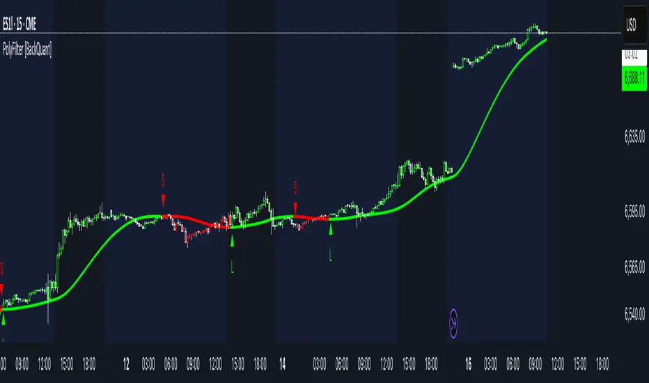
PolyFilter [BackQuant]PolyFilter
A flexible, low-lag trend filter with three smoothing engines—optimized for clean bias, fewer whipsaws, and clear alerting.
What it does
PolyFilter draws a single “intelligent” baseline that adapts to price while suppressing noise. You choose the engine— Fractional MA , Ehlers 2-Pole Super Smoother , or a Multi-Kernel blend . The line can color itself by slope (trend) or by position vs price (above/below), and you get four ready-made alerts for flips and crosses.
What it plots
PolyFilter line — your smoothed trend baseline (width set by “Line Width”).
Optional candle & background coloring — choose: color by trend slope or by whether price is above/below the filter.
Signal markers — Arrows with L/S when the slope flips or when price crosses the line (if you enable shapes/alerts).
How the three engines differ
Fractional MA (experimental) — A power-law weighting of past bars (heavier focus on the most recent samples without throwing away history). The Adaptation Speed acts like the “fraction” exponent (default 0.618). Lower values lean more on recent bars; higher values spread weight further back.
Ehlers 2-Pole Super Smoother — Classic low-lag IIR smoother that aggressively reduces high-frequency noise while preserving turns. Great default when you want a steady, responsive baseline with minimal parameter fuss.
Multi-Kernel — A 70/30 blend of a Gaussian window and an exponential kernel. The Gaussian contributes smooth structure; the exponential adds a hint of responsiveness. Useful for assets that oscillate but still trend.
Reading the colors
Trend mode (default) — Line & candles turn green while the filter is rising (signal > signal ) and red while it’s falling.
Above/Below mode — Line & candles reflect price’s position relative to the filter: green when price > filter, red when price < filter. This is handy if you treat the filter like a dynamic “fair value” or bias line.
Inputs you’ll actually use
Calculation Settings
Price Source — Default HLC/3. Switch to Close for stricter trend, or HLC3/HL2 to soften single-print spikes.
Filter Length — Window/period for all engines. Shorter = snappier turns; longer = smoother line.
Adaptation Speed — Only affects Fractional MA . Lower it for faster, more local weighting; raise it for smoother, more global weighting.
Filter Type — Pick one of: Fractional MA, Ehlers 2-Pole, Multi-Kernel.
UI & Plotting
Color based off… — Choose Trend (slope) or > or < Close (position vs price).
Long/Short Colors — Customize bull/bear hues to your theme.
Show Filter Line / Paint candles / Color background — Visual toggles for the line, bars, and backdrop.
Line Width — Make the filter stand out (2–3 works well on most charts).
Signals & Alerts
PolyFilter Trend Up — Slope flips upward (the filter crosses above its prior value). Good for early continuation entries or stop-tightening on shorts.
PolyFilter Trend Down — Slope flips downward. Often used to scale out longs or rotate bias.
PolyFilter Above Price — The filter line crosses up through price (filter > price). This can confirm that mean has “caught up” after a pullback.
PolyFilter Below Price — The filter line crosses down through price (filter < price). Useful to confirm momentum loss on bounces.
Quick starts (suggested presets)
Intraday (5–15m, crypto or indices) — Ehlers 2-Pole, Length 55–80. Trend coloring ON, candle paint ON. Look for pullbacks to a rising filter; avoid fading a falling one.
Swing (1H–4H) — Multi-Kernel, Length 80–120. Background color OFF (cleaner), candle paint ON. Add a higher-TF confirmation (e.g., 4H filter rising when you trade 1H).
Range-prone FX — Fractional MA, Length 70–100, Adaptation ~0.55–0.70. Consider Above/Below mode to trade mean reversion to the line with a strict risk cap.
How to use it in practice
Bias line — Trade in the direction of the filter slope; stand aside when it flattens and color chops back and forth.
Dynamic support/resistance — Treat the line as a moving value area. In trends, entries often appear on shallow tags of the line with structure confluence.
Regime switch — When the filter flips and holds color for several bars, tighten stops on the opposing side and look for first pullback in the new color.
Stacking filters — Many users run PolyFilter on the active chart and a slower instance (longer length) on a higher timeframe as a “macro bias” guardrail.
Tuning tips
If you see too many flips, lengthen the filter or switch to Multi-Kernel.
If turns feel late, shorten the filter or try Ehlers 2-Pole for lower lag.
On thin or very noisy symbols, prefer HLC3 as the source and longer lengths.
Performance note: very large lengths increase computation time for the Multi-Kernel and Fractional engines. Start moderate and scale up only if needed.
Summary
PolyFilter gives you a single, trustworthy baseline that you can read at a glance—either as a pure trend line (slope coloring) or as a dynamic “above/below fair value” reference. Pick the engine that matches your market’s personality, set a sensible length, and let the color and alerts guide bias, entries on pullbacks, and risk on reversals.
Tzotchev Trend Measure [EdgeTools]Are you still measuring trend strength with moving averages? Here is a better variant at scientific level:
Tzotchev Trend Measure: A Statistical Approach to Trend Following
The Tzotchev Trend Measure represents a sophisticated advancement in quantitative trend analysis, moving beyond traditional moving average-based indicators toward a statistically rigorous framework for measuring trend strength. This indicator implements the methodology developed by Tzotchev et al. (2015) in their seminal J.P. Morgan research paper "Designing robust trend-following system: Behind the scenes of trend-following," which introduced a probabilistic approach to trend measurement that has since become a cornerstone of institutional trading strategies.
Mathematical Foundation and Statistical Theory
The core innovation of the Tzotchev Trend Measure lies in its transformation of price momentum into a probability-based metric through the application of statistical hypothesis testing principles. The indicator employs the fundamental formula ST = 2 × Φ(√T × r̄T / σ̂T) - 1, where ST represents the trend strength score bounded between -1 and +1, Φ(x) denotes the normal cumulative distribution function, T represents the lookback period in trading days, r̄T is the average logarithmic return over the specified period, and σ̂T represents the estimated daily return volatility.
This formulation transforms what is essentially a t-statistic into a probabilistic trend measure, testing the null hypothesis that the mean return equals zero against the alternative hypothesis of non-zero mean return. The use of logarithmic returns rather than simple returns provides several statistical advantages, including symmetry properties where log(P₁/P₀) = -log(P₀/P₁), additivity characteristics that allow for proper compounding analysis, and improved validity of normal distribution assumptions that underpin the statistical framework.
The implementation utilizes the Abramowitz and Stegun (1964) approximation for the normal cumulative distribution function, achieving accuracy within ±1.5 × 10⁻⁷ for all input values. This approximation employs Horner's method for polynomial evaluation to ensure numerical stability, particularly important when processing large datasets or extreme market conditions.
Comparative Analysis with Traditional Trend Measurement Methods
The Tzotchev Trend Measure demonstrates significant theoretical and empirical advantages over conventional trend analysis techniques. Traditional moving average-based systems, including simple moving averages (SMA), exponential moving averages (EMA), and their derivatives such as MACD, suffer from several fundamental limitations that the Tzotchev methodology addresses systematically.
Moving average systems exhibit inherent lag bias, as documented by Kaufman (2013) in "Trading Systems and Methods," where he demonstrates that moving averages inevitably lag price movements by approximately half their period length. This lag creates delayed signal generation that reduces profitability in trending markets and increases false signal frequency during consolidation periods. In contrast, the Tzotchev measure eliminates lag bias by directly analyzing the statistical properties of return distributions rather than smoothing price levels.
The volatility normalization inherent in the Tzotchev formula addresses a critical weakness in traditional momentum indicators. As shown by Bollinger (2001) in "Bollinger on Bollinger Bands," momentum oscillators like RSI and Stochastic fail to account for changing volatility regimes, leading to inconsistent signal interpretation across different market conditions. The Tzotchev measure's incorporation of return volatility in the denominator ensures that trend strength assessments remain consistent regardless of the underlying volatility environment.
Empirical studies by Hurst, Ooi, and Pedersen (2013) in "Demystifying Managed Futures" demonstrate that traditional trend-following indicators suffer from significant drawdowns during whipsaw markets, with Sharpe ratios frequently below 0.5 during challenging periods. The authors attribute these poor performance characteristics to the binary nature of most trend signals and their inability to quantify signal confidence. The Tzotchev measure addresses this limitation by providing continuous probability-based outputs that allow for more sophisticated risk management and position sizing strategies.
The statistical foundation of the Tzotchev approach provides superior robustness compared to technical indicators that lack theoretical grounding. Fama and French (1988) in "Permanent and Temporary Components of Stock Prices" established that price movements contain both permanent and temporary components, with traditional moving averages unable to distinguish between these elements effectively. The Tzotchev methodology's hypothesis testing framework specifically tests for the presence of permanent trend components while filtering out temporary noise, providing a more theoretically sound approach to trend identification.
Research by Moskowitz, Ooi, and Pedersen (2012) in "Time Series Momentum in the Cross Section of Asset Returns" found that traditional momentum indicators exhibit significant variation in effectiveness across asset classes and time periods. Their study of multiple asset classes over decades revealed that simple price-based momentum measures often fail to capture persistent trends in fixed income and commodity markets. The Tzotchev measure's normalization by volatility and its probabilistic interpretation provide consistent performance across diverse asset classes, as demonstrated in the original J.P. Morgan research.
Comparative performance studies conducted by AQR Capital Management (Asness, Moskowitz, and Pedersen, 2013) in "Value and Momentum Everywhere" show that volatility-adjusted momentum measures significantly outperform traditional price momentum across international equity, bond, commodity, and currency markets. The study documents Sharpe ratio improvements of 0.2 to 0.4 when incorporating volatility normalization, consistent with the theoretical advantages of the Tzotchev approach.
The regime detection capabilities of the Tzotchev measure provide additional advantages over binary trend classification systems. Research by Ang and Bekaert (2002) in "Regime Switches in Interest Rates" demonstrates that financial markets exhibit distinct regime characteristics that traditional indicators fail to capture adequately. The Tzotchev measure's five-tier classification system (Strong Bull, Weak Bull, Neutral, Weak Bear, Strong Bear) provides more nuanced market state identification than simple trend/no-trend binary systems.
Statistical testing by Jegadeesh and Titman (2001) in "Profitability of Momentum Strategies" revealed that traditional momentum indicators suffer from significant parameter instability, with optimal lookback periods varying substantially across market conditions and asset classes. The Tzotchev measure's statistical framework provides more stable parameter selection through its grounding in hypothesis testing theory, reducing the need for frequent parameter optimization that can lead to overfitting.
Advanced Noise Filtering and Market Regime Detection
A significant enhancement over the original Tzotchev methodology is the incorporation of a multi-factor noise filtering system designed to reduce false signals during sideways market conditions. The filtering mechanism employs four distinct approaches: adaptive thresholding based on current market regime strength, volatility-based filtering utilizing ATR percentile analysis, trend strength confirmation through momentum alignment, and a comprehensive multi-factor approach that combines all methodologies.
The adaptive filtering system analyzes market microstructure through price change relative to average true range, calculates volatility percentiles over rolling windows, and assesses trend alignment across multiple timeframes using exponential moving averages of varying periods. This approach addresses one of the primary limitations identified in traditional trend-following systems, namely their tendency to generate excessive false signals during periods of low volatility or sideways price action.
The regime detection component classifies market conditions into five distinct categories: Strong Bull (ST > 0.3), Weak Bull (0.1 < ST ≤ 0.3), Neutral (-0.1 ≤ ST ≤ 0.1), Weak Bear (-0.3 ≤ ST < -0.1), and Strong Bear (ST < -0.3). This classification system provides traders with clear, quantitative definitions of market regimes that can inform position sizing, risk management, and strategy selection decisions.
Professional Implementation and Trading Applications
The indicator incorporates three distinct trading profiles designed to accommodate different investment approaches and risk tolerances. The Conservative profile employs longer lookback periods (63 days), higher signal thresholds (0.2), and reduced filter sensitivity (0.5) to minimize false signals and focus on major trend changes. The Balanced profile utilizes standard academic parameters with moderate settings across all dimensions. The Aggressive profile implements shorter lookback periods (14 days), lower signal thresholds (-0.1), and increased filter sensitivity (1.5) to capture shorter-term trend movements.
Signal generation occurs through threshold crossover analysis, where long signals are generated when the trend measure crosses above the specified threshold and short signals when it crosses below. The implementation includes sophisticated signal confirmation mechanisms that consider trend alignment across multiple timeframes and momentum strength percentiles to reduce the likelihood of false breakouts.
The alert system provides real-time notifications for trend threshold crossovers, strong regime changes, and signal generation events, with configurable frequency controls to prevent notification spam. Alert messages are standardized to ensure consistency across different market conditions and timeframes.
Performance Optimization and Computational Efficiency
The implementation incorporates several performance optimization features designed to handle large datasets efficiently. The maximum bars back parameter allows users to control historical calculation depth, with default settings optimized for most trading applications while providing flexibility for extended historical analysis. The system includes automatic performance monitoring that generates warnings when computational limits are approached.
Error handling mechanisms protect against division by zero conditions, infinite values, and other numerical instabilities that can occur during extreme market conditions. The finite value checking system ensures data integrity throughout the calculation process, with fallback mechanisms that maintain indicator functionality even when encountering corrupted or missing price data.
Timeframe validation provides warnings when the indicator is applied to unsuitable timeframes, as the Tzotchev methodology was specifically designed for daily and higher timeframe analysis. This validation helps prevent misapplication of the indicator in contexts where its statistical assumptions may not hold.
Visual Design and User Interface
The indicator features eight professional color schemes designed for different trading environments and user preferences. The EdgeTools theme provides an institutional blue and steel color palette suitable for professional trading environments. The Gold theme offers warm colors optimized for commodities trading. The Behavioral theme incorporates psychology-based color contrasts that align with behavioral finance principles. The Quant theme provides neutral colors suitable for analytical applications.
Additional specialized themes include Ocean, Fire, Matrix, and Arctic variations, each optimized for specific visual preferences and trading contexts. All color schemes include automatic dark and light mode optimization to ensure optimal readability across different chart backgrounds and trading platforms.
The information table provides real-time display of key metrics including current trend measure value, market regime classification, signal strength, Z-score, average returns, volatility measures, filter threshold levels, and filter effectiveness percentages. This comprehensive dashboard allows traders to monitor all relevant indicator components simultaneously.
Theoretical Implications and Research Context
The Tzotchev Trend Measure addresses several theoretical limitations inherent in traditional technical analysis approaches. Unlike moving average-based systems that rely on price level comparisons, this methodology grounds trend analysis in statistical hypothesis testing, providing a more robust theoretical foundation for trading decisions.
The probabilistic interpretation of trend strength offers significant advantages over binary trend classification systems. Rather than simply indicating whether a trend exists, the measure quantifies the statistical confidence level associated with the trend assessment, allowing for more nuanced risk management and position sizing decisions.
The incorporation of volatility normalization addresses the well-documented problem of volatility clustering in financial time series, ensuring that trend strength assessments remain consistent across different market volatility regimes. This normalization is particularly important for portfolio management applications where consistent risk metrics across different assets and time periods are essential.
Practical Applications and Trading Strategy Integration
The Tzotchev Trend Measure can be effectively integrated into various trading strategies and portfolio management frameworks. For trend-following strategies, the indicator provides clear entry and exit signals with quantified confidence levels. For mean reversion strategies, extreme readings can signal potential turning points. For portfolio allocation, the regime classification system can inform dynamic asset allocation decisions.
The indicator's statistical foundation makes it particularly suitable for quantitative trading strategies where systematic, rules-based approaches are preferred over discretionary decision-making. The standardized output range facilitates easy integration with position sizing algorithms and risk management systems.
Risk management applications benefit from the indicator's ability to quantify trend strength and provide early warning signals of potential trend changes. The multi-timeframe analysis capability allows for the construction of robust risk management frameworks that consider both short-term tactical and long-term strategic market conditions.
Implementation Guide and Parameter Configuration
The practical application of the Tzotchev Trend Measure requires careful parameter configuration to optimize performance for specific trading objectives and market conditions. This section provides comprehensive guidance for parameter selection and indicator customization.
Core Calculation Parameters
The Lookback Period parameter controls the statistical window used for trend calculation and represents the most critical setting for the indicator. Default values range from 14 to 63 trading days, with shorter periods (14-21 days) providing more sensitive trend detection suitable for short-term trading strategies, while longer periods (42-63 days) offer more stable trend identification appropriate for position trading and long-term investment strategies. The parameter directly influences the statistical significance of trend measurements, with longer periods requiring stronger underlying trends to generate significant signals but providing greater reliability in trend identification.
The Price Source parameter determines which price series is used for return calculations. The default close price provides standard trend analysis, while alternative selections such as high-low midpoint ((high + low) / 2) can reduce noise in volatile markets, and volume-weighted average price (VWAP) offers superior trend identification in institutional trading environments where volume concentration matters significantly.
The Signal Threshold parameter establishes the minimum trend strength required for signal generation, with values ranging from -0.5 to 0.5. Conservative threshold settings (0.2 to 0.3) reduce false signals but may miss early trend opportunities, while aggressive settings (-0.1 to 0.1) provide earlier signal generation at the cost of increased false positive rates. The optimal threshold depends on the trader's risk tolerance and the volatility characteristics of the traded instrument.
Trading Profile Configuration
The Trading Profile system provides pre-configured parameter sets optimized for different trading approaches. The Conservative profile employs a 63-day lookback period with a 0.2 signal threshold and 0.5 noise sensitivity, designed for long-term position traders seeking high-probability trend signals with minimal false positives. The Balanced profile uses a 21-day lookback with 0.05 signal threshold and 1.0 noise sensitivity, suitable for swing traders requiring moderate signal frequency with acceptable noise levels. The Aggressive profile implements a 14-day lookback with -0.1 signal threshold and 1.5 noise sensitivity, optimized for day traders and scalpers requiring frequent signal generation despite higher noise levels.
Advanced Noise Filtering System
The noise filtering mechanism addresses the challenge of false signals during sideways market conditions through four distinct methodologies. The Adaptive filter adjusts thresholds based on current trend strength, increasing sensitivity during strong trending periods while raising thresholds during consolidation phases. The Volatility-based filter utilizes Average True Range (ATR) percentile analysis to suppress signals during abnormally volatile conditions that typically generate false trend indications.
The Trend Strength filter requires alignment between multiple momentum indicators before confirming signals, reducing the probability of false breakouts from consolidation patterns. The Multi-factor approach combines all filtering methodologies using weighted scoring to provide the most robust noise reduction while maintaining signal responsiveness during genuine trend initiations.
The Noise Sensitivity parameter controls the aggressiveness of the filtering system, with lower values (0.5-1.0) providing conservative filtering suitable for volatile instruments, while higher values (1.5-2.0) allow more signals through but may increase false positive rates during choppy market conditions.
Visual Customization and Display Options
The Color Scheme parameter offers eight professional visualization options designed for different analytical preferences and market conditions. The EdgeTools scheme provides high contrast visualization optimized for trend strength differentiation, while the Gold scheme offers warm tones suitable for commodity analysis. The Behavioral scheme uses psychological color associations to enhance decision-making speed, and the Quant scheme provides neutral colors appropriate for quantitative analysis environments.
The Ocean, Fire, Matrix, and Arctic schemes offer additional aesthetic options while maintaining analytical functionality. Each scheme includes optimized colors for both light and dark chart backgrounds, ensuring visibility across different trading platform configurations.
The Show Glow Effects parameter enhances plot visibility through multiple layered lines with progressive transparency, particularly useful when analyzing multiple timeframes simultaneously or when working with dense price data that might obscure trend signals.
Performance Optimization Settings
The Maximum Bars Back parameter controls the historical data depth available for calculations, with values ranging from 5,000 to 50,000 bars. Higher values enable analysis of longer-term trend patterns but may impact indicator loading speed on slower systems or when applied to multiple instruments simultaneously. The optimal setting depends on the intended analysis timeframe and available computational resources.
The Calculate on Every Tick parameter determines whether the indicator updates with every price change or only at bar close. Real-time calculation provides immediate signal updates suitable for scalping and day trading strategies, while bar-close calculation reduces computational overhead and eliminates signal flickering during bar formation, preferred for swing trading and position management applications.
Alert System Configuration
The Alert Frequency parameter controls notification generation, with options for all signals, bar close only, or once per bar. High-frequency trading strategies benefit from all signals mode, while position traders typically prefer bar close alerts to avoid premature position entries based on intrabar fluctuations.
The alert system generates four distinct notification types: Long Signal alerts when the trend measure crosses above the positive signal threshold, Short Signal alerts for negative threshold crossings, Bull Regime alerts when entering strong bullish conditions, and Bear Regime alerts for strong bearish regime identification.
Table Display and Information Management
The information table provides real-time statistical metrics including current trend value, regime classification, signal status, and filter effectiveness measurements. The table position can be customized for optimal screen real estate utilization, and individual metrics can be toggled based on analytical requirements.
The Language parameter supports both English and German display options for international users, while maintaining consistent calculation methodology regardless of display language selection.
Risk Management Integration
Effective risk management integration requires coordination between the trend measure signals and position sizing algorithms. Strong trend readings (above 0.5 or below -0.5) support larger position sizes due to higher probability of trend continuation, while neutral readings (between -0.2 and 0.2) suggest reduced position sizes or range-trading strategies.
The regime classification system provides additional risk management context, with Strong Bull and Strong Bear regimes supporting trend-following strategies, while Neutral regimes indicate potential for mean reversion approaches. The filter effectiveness metric helps traders assess current market conditions and adjust strategy parameters accordingly.
Timeframe Considerations and Multi-Timeframe Analysis
The indicator's effectiveness varies across different timeframes, with higher timeframes (daily, weekly) providing more reliable trend identification but slower signal generation, while lower timeframes (hourly, 15-minute) offer faster signals with increased noise levels. Multi-timeframe analysis combining trend alignment across multiple periods significantly improves signal quality and reduces false positive rates.
For optimal results, traders should consider trend alignment between the primary trading timeframe and at least one higher timeframe before entering positions. Divergences between timeframes often signal potential trend reversals or consolidation periods requiring strategy adjustment.
Conclusion
The Tzotchev Trend Measure represents a significant advancement in technical analysis methodology, combining rigorous statistical foundations with practical trading applications. Its implementation of the J.P. Morgan research methodology provides institutional-quality trend analysis capabilities previously available only to sophisticated quantitative trading firms.
The comprehensive parameter configuration options enable customization for diverse trading styles and market conditions, while the advanced noise filtering and regime detection capabilities provide superior signal quality compared to traditional trend-following indicators. Proper parameter selection and understanding of the indicator's statistical foundation are essential for achieving optimal trading results and effective risk management.
References
Abramowitz, M. and Stegun, I.A. (1964). Handbook of Mathematical Functions with Formulas, Graphs, and Mathematical Tables. Washington: National Bureau of Standards.
Ang, A. and Bekaert, G. (2002). Regime Switches in Interest Rates. Journal of Business and Economic Statistics, 20(2), 163-182.
Asness, C.S., Moskowitz, T.J., and Pedersen, L.H. (2013). Value and Momentum Everywhere. Journal of Finance, 68(3), 929-985.
Bollinger, J. (2001). Bollinger on Bollinger Bands. New York: McGraw-Hill.
Fama, E.F. and French, K.R. (1988). Permanent and Temporary Components of Stock Prices. Journal of Political Economy, 96(2), 246-273.
Hurst, B., Ooi, Y.H., and Pedersen, L.H. (2013). Demystifying Managed Futures. Journal of Investment Management, 11(3), 42-58.
Jegadeesh, N. and Titman, S. (2001). Profitability of Momentum Strategies: An Evaluation of Alternative Explanations. Journal of Finance, 56(2), 699-720.
Kaufman, P.J. (2013). Trading Systems and Methods. 5th Edition. Hoboken: John Wiley & Sons.
Moskowitz, T.J., Ooi, Y.H., and Pedersen, L.H. (2012). Time Series Momentum. Journal of Financial Economics, 104(2), 228-250.
Tzotchev, D., Lo, A.W., and Hasanhodzic, J. (2015). Designing robust trend-following system: Behind the scenes of trend-following. J.P. Morgan Quantitative Research, Asset Management Division.

EMA vs TMA Regime FilterEMA vs TMA Regime Filter
This indicator is built as a visual study tool to compare the behavior of the Exponential Moving Average (EMA) and the Triangular Moving Average (TMA).
The EMA applies an exponential weighting to price data, giving stronger importance to the most recent values. This makes it a faster, more responsive line that reflects short-term momentum. The TMA, by contrast, applies a double-smoothing process (or in the “True TMA” option, a split SMA sequence), which produces a much slower curve. The TMA emphasizes balance over reactivity, often used for filtering noise and observing longer-term structure.
When both are plotted on the same chart, their differences become clear. The shaded region between them highlights times when short-term price dynamics diverge from longer-term smoothing. This is where the idea of “regime” comes in — not as a trading signal, but as a descriptive way of seeing whether market action is currently dominated by speed or by stability.
Users can customize:
Line styles, widths, and colors.
Cloud transparency for visual clarity.
Whether to color bars based on relative position (optional, purely visual).
The goal is not to create a system, but to help traders experiment, observe, and learn how different smoothing techniques can emphasize different aspects of price. By switching between the legacy and true TMA, or adjusting lengths, users can study how each approach interprets the same data differently.
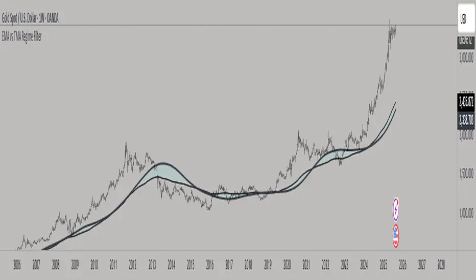
On-Balance Volume with Multiple MA TypesOn-Balance Volume with Multiple MA Types
English Description
Overview
This is the first version of the "On-Balance Volume with Multiple MA Types" indicator designed to overlay directly on the price chart, a significant evolution from its previous iterations, which functioned solely as an oscillator in a separate window. The indicator calculates On-Balance Volume (OBV) and applies various smoothing methods to provide a clear view of volume dynamics in relation to price movements. It is pinned to the price scale for seamless integration with the chart.
Interpretation Recommendations
Price Pushing the OBV Line from Below: When the price chart pushes the OBV line upward and remains below it, this indicates rising volume, suggesting strong buying pressure.
Price Above the OBV Line: When the price chart is above the OBV line, it signals falling volume, indicating weakening momentum or selling pressure.
OBV Line Crossings: When the price crosses the OBV line, it represents a balance point in volume dynamics. The price level at the current crossing can be compared to the previous crossing to assess changes in market sentiment or momentum.
Moving Average Types
The indicator offers eight smoothing options for the OBV line, each with unique characteristics:
EMA (Exponential Moving Average): A weighted average that prioritizes recent data, providing a smooth yet responsive line.
DEMA (Double Exponential Moving Average): Uses two EMAs to reduce lag, offering faster response to volume changes.
HMA (Hull Moving Average): Combines weighted moving averages to minimize lag while maintaining smoothness.
WMA (Weighted Moving Average): Assigns more weight to recent data, balancing responsiveness and noise reduction.
TMA (Triangular Moving Average): A double-smoothed simple moving average, emphasizing central data points for smoother output.
VIDYA (Variable Index Dynamic Average): Adapts smoothing based on market volatility, using a CMO (Chande Momentum Oscillator) for dynamic weighting. Controlled by the VIDYA Alpha parameter (default: 0.2, range: 0–1), which adjusts sensitivity to volatility.
FRAMA (Fractal Adaptive Moving Average): Adjusts smoothing based on fractal dimensions of the OBV data, adapting to market conditions.
JMA (Jurik Moving Average): A proprietary adaptive average designed for minimal lag and high smoothness. Controlled by two parameters:
JMA Phase (default: 50, range: -100 to 100): Adjusts the balance between responsiveness and smoothness.
JMA Power (default: 1, range: 0.1+): Controls the strength of smoothing.
Input Parameters
OBV MA Length (default: 10): The lookback period for smoothing the OBV. Higher values produce smoother results but increase lag.
OBV MA Type (default: JMA): Selects the moving average type from the eight options listed above.
Line Width (default: 2): Thickness of the OBV line on the chart.
Bullish Color (default: Blue): Color of the OBV line when rising (indicating increasing volume).
Bearish Color (default: Red): Color of the OBV line when falling (indicating decreasing volume).
JMA Phase (default: 50): Adjusts the JMA’s responsiveness (used only when JMA is selected).
JMA Power (default: 1): Adjusts the JMA’s smoothing strength (used only when JMA is selected).
VIDYA Alpha (default: 0.2): Controls the sensitivity of VIDYA to market volatility (used only when VIDYA is selected).
How to Use
Add the indicator to your TradingView chart. It will overlay directly on the price chart, aligned with the price scale.
Adjust the OBV MA Type to select your preferred smoothing method based on your trading style (e.g., JMA for low lag, TMA for smoothness).
Modify the OBV MA Length to balance responsiveness and noise reduction. Shorter periods (e.g., 5–10) are better for short-term trading, while longer periods (e.g., 20–50) suit longer-term analysis.
Use the Bullish Color and Bearish Color to visually distinguish rising and falling volume trends.
For JMA or VIDYA, fine-tune the JMA Phase, JMA Power, or VIDYA Alpha to optimize the indicator for specific market conditions.
Interpret the OBV line in relation to price:
Watch for price pushing the OBV line upward (rising volume) or moving above it (falling volume).
Note crossings of the OBV line to identify balance points and compare with prior crossings to gauge momentum shifts.
Combine with other technical tools (e.g., support/resistance levels, trendlines) for a comprehensive trading strategy.
Notes
This indicator is designed to work on any timeframe and market, but its effectiveness depends on the chosen moving average type and parameters.
Experiment with different MA types and lengths to find the best fit for your trading approach.
The indicator is licensed under the Mozilla Public License 2.0 and copyrighted by TradingStrategyCourses © 2025.

Trend CandlesTrend Candles
Overview
The Trend Candles indicator is a simple yet effective tool designed to help traders visually identify the prevailing market trend. By combining candle coloring with a trend-based Exponential Moving Average (EMA), it enhances chart readability and makes trend-following strategies easier to apply.
Concepts
Exponential Moving Average (EMA): The EMA is a moving average that places more weight on recent price data. It reacts faster to price changes compared to a Simple Moving Average (SMA), making it well-suited for trend detection.
Trend Determination:
- If the EMA is rising (current EMA > previous EMA), the market is considered bullish.
- If the EMA is falling (current EMA < previous EMA), the market is considered bearish.
- If the EMA is flat (no significant change), no trend color is applied.
Candle Coloring:
- Green candles = Uptrend
- Purple candles = Downtrend
- Default candles = Sideways/Flat EMA
Features
- Trend Visualization: Candles automatically change color based on EMA slope, making it easy to spot bullish and bearish phases.
- Customizable EMA Length: The trader can set the EMA period (default is 50), allowing flexibility for short-term or long-term trend analysis.
- Overlay EMA Line: An orange EMA line is plotted on the chart for additional confirmation of the trend.
- Clean & Minimalist: Focuses on trend clarity without cluttering the chart with unnecessary signals.
How to Use
1. Apply the indicator to your chart.
2. Adjust the EMA Length as per your trading style (shorter = faster signals, longer = smoother trend).
3. Follow the candle color:
- Green = Favor long entries.
- Purple = Favor short entries.
- No color = Stay cautious, as trend is unclear.
4. Use with other confirmation tools (support/resistance, volume, or oscillators).
5. Users are encouraged to experiment with different EMA lengths. The default length is 50, but you can explore other values based on your needs. In particular, try Fibonacci numbers such as 13, 21, 34, 55, 89, 144, and 233 to observe how trends behave differently.
Disclaimer
The information provided by the Trend Candles indicator is for educational purposes only. It should not be considered financial advice. Trading involves substantial risk, and past performance is not necessarily indicative of future results. Always do your own research and use risk management practices.

Markov Chain [3D] | FractalystWhat exactly is a Markov Chain?
This indicator uses a Markov Chain model to analyze, quantify, and visualize the transitions between market regimes (Bull, Bear, Neutral) on your chart. It dynamically detects these regimes in real-time, calculates transition probabilities, and displays them as animated 3D spheres and arrows, giving traders intuitive insight into current and future market conditions.
How does a Markov Chain work, and how should I read this spheres-and-arrows diagram?
Think of three weather modes: Sunny, Rainy, Cloudy.
Each sphere is one mode. The loop on a sphere means “stay the same next step” (e.g., Sunny again tomorrow).
The arrows leaving a sphere show where things usually go next if they change (e.g., Sunny moving to Cloudy).
Some paths matter more than others. A more prominent loop means the current mode tends to persist. A more prominent outgoing arrow means a change to that destination is the usual next step.
Direction isn’t symmetric: moving Sunny→Cloudy can behave differently than Cloudy→Sunny.
Now relabel the spheres to markets: Bull, Bear, Neutral.
Spheres: market regimes (uptrend, downtrend, range).
Self‑loop: tendency for the current regime to continue on the next bar.
Arrows: the most common next regime if a switch happens.
How to read: Start at the sphere that matches current bar state. If the loop stands out, expect continuation. If one outgoing path stands out, that switch is the typical next step. Opposite directions can differ (Bear→Neutral doesn’t have to match Neutral→Bear).
What states and transitions are shown?
The three market states visualized are:
Bullish (Bull): Upward or strong-market regime.
Bearish (Bear): Downward or weak-market regime.
Neutral: Sideways or range-bound regime.
Bidirectional animated arrows and probability labels show how likely the market is to move from one regime to another (e.g., Bull → Bear or Neutral → Bull).
How does the regime detection system work?
You can use either built-in price returns (based on adaptive Z-score normalization) or supply three custom indicators (such as volume, oscillators, etc.).
Values are statistically normalized (Z-scored) over a configurable lookback period.
The normalized outputs are classified into Bull, Bear, or Neutral zones.
If using three indicators, their regime signals are averaged and smoothed for robustness.
How are transition probabilities calculated?
On every confirmed bar, the algorithm tracks the sequence of detected market states, then builds a rolling window of transitions.
The code maintains a transition count matrix for all regime pairs (e.g., Bull → Bear).
Transition probabilities are extracted for each possible state change using Laplace smoothing for numerical stability, and frequently updated in real-time.
What is unique about the visualization?
3D animated spheres represent each regime and change visually when active.
Animated, bidirectional arrows reveal transition probabilities and allow you to see both dominant and less likely regime flows.
Particles (moving dots) animate along the arrows, enhancing the perception of regime flow direction and speed.
All elements dynamically update with each new price bar, providing a live market map in an intuitive, engaging format.
Can I use custom indicators for regime classification?
Yes! Enable the "Custom Indicators" switch and select any three chart series as inputs. These will be normalized and combined (each with equal weight), broadening the regime classification beyond just price-based movement.
What does the “Lookback Period” control?
Lookback Period (default: 100) sets how much historical data builds the probability matrix. Shorter periods adapt faster to regime changes but may be noisier. Longer periods are more stable but slower to adapt.
How is this different from a Hidden Markov Model (HMM)?
It sets the window for both regime detection and probability calculations. Lower values make the system more reactive, but potentially noisier. Higher values smooth estimates and make the system more robust.
How is this Markov Chain different from a Hidden Markov Model (HMM)?
Markov Chain (as here): All market regimes (Bull, Bear, Neutral) are directly observable on the chart. The transition matrix is built from actual detected regimes, keeping the model simple and interpretable.
Hidden Markov Model: The actual regimes are unobservable ("hidden") and must be inferred from market output or indicator "emissions" using statistical learning algorithms. HMMs are more complex, can capture more subtle structure, but are harder to visualize and require additional machine learning steps for training.
A standard Markov Chain models transitions between observable states using a simple transition matrix, while a Hidden Markov Model assumes the true states are hidden (latent) and must be inferred from observable “emissions” like price or volume data. In practical terms, a Markov Chain is transparent and easier to implement and interpret; an HMM is more expressive but requires statistical inference to estimate hidden states from data.
Markov Chain: states are observable; you directly count or estimate transition probabilities between visible states. This makes it simpler, faster, and easier to validate and tune.
HMM: states are hidden; you only observe emissions generated by those latent states. Learning involves machine learning/statistical algorithms (commonly Baum–Welch/EM for training and Viterbi for decoding) to infer both the transition dynamics and the most likely hidden state sequence from data.
How does the indicator avoid “repainting” or look-ahead bias?
All regime changes and matrix updates happen only on confirmed (closed) bars, so no future data is leaked, ensuring reliable real-time operation.
Are there practical tuning tips?
Tune the Lookback Period for your asset/timeframe: shorter for fast markets, longer for stability.
Use custom indicators if your asset has unique regime drivers.
Watch for rapid changes in transition probabilities as early warning of a possible regime shift.
Who is this indicator for?
Quants and quantitative researchers exploring probabilistic market modeling, especially those interested in regime-switching dynamics and Markov models.
Programmers and system developers who need a probabilistic regime filter for systematic and algorithmic backtesting:
The Markov Chain indicator is ideally suited for programmatic integration via its bias output (1 = Bull, 0 = Neutral, -1 = Bear).
Although the visualization is engaging, the core output is designed for automated, rules-based workflows—not for discretionary/manual trading decisions.
Developers can connect the indicator’s output directly to their Pine Script logic (using input.source()), allowing rapid and robust backtesting of regime-based strategies.
It acts as a plug-and-play regime filter: simply plug the bias output into your entry/exit logic, and you have a scientifically robust, probabilistically-derived signal for filtering, timing, position sizing, or risk regimes.
The MC's output is intentionally "trinary" (1/0/-1), focusing on clear regime states for unambiguous decision-making in code. If you require nuanced, multi-probability or soft-label state vectors, consider expanding the indicator or stacking it with a probability-weighted logic layer in your scripting.
Because it avoids subjectivity, this approach is optimal for systematic quants, algo developers building backtested, repeatable strategies based on probabilistic regime analysis.
What's the mathematical foundation behind this?
The mathematical foundation behind this Markov Chain indicator—and probabilistic regime detection in finance—draws from two principal models: the (standard) Markov Chain and the Hidden Markov Model (HMM).
How to use this indicator programmatically?
The Markov Chain indicator automatically exports a bias value (+1 for Bullish, -1 for Bearish, 0 for Neutral) as a plot visible in the Data Window. This allows you to integrate its regime signal into your own scripts and strategies for backtesting, automation, or live trading.
Step-by-Step Integration with Pine Script (input.source)
Add the Markov Chain indicator to your chart.
This must be done first, since your custom script will "pull" the bias signal from the indicator's plot.
In your strategy, create an input using input.source()
Example:
//@version=5
strategy("MC Bias Strategy Example")
mcBias = input.source(close, "MC Bias Source")
After saving, go to your script’s settings. For the “MC Bias Source” input, select the plot/output of the Markov Chain indicator (typically its bias plot).
Use the bias in your trading logic
Example (long only on Bull, flat otherwise):
if mcBias == 1
strategy.entry("Long", strategy.long)
else
strategy.close("Long")
For more advanced workflows, combine mcBias with additional filters or trailing stops.
How does this work behind-the-scenes?
TradingView’s input.source() lets you use any plot from another indicator as a real-time, “live” data feed in your own script (source).
The selected bias signal is available to your Pine code as a variable, enabling logical decisions based on regime (trend-following, mean-reversion, etc.).
This enables powerful strategy modularity : decouple regime detection from entry/exit logic, allowing fast experimentation without rewriting core signal code.
Integrating 45+ Indicators with Your Markov Chain — How & Why
The Enhanced Custom Indicators Export script exports a massive suite of over 45 technical indicators—ranging from classic momentum (RSI, MACD, Stochastic, etc.) to trend, volume, volatility, and oscillator tools—all pre-calculated, centered/scaled, and available as plots.
// Enhanced Custom Indicators Export - 45 Technical Indicators
// Comprehensive technical analysis suite for advanced market regime detection
//@version=6
indicator('Enhanced Custom Indicators Export | Fractalyst', shorttitle='Enhanced CI Export', overlay=false, scale=scale.right, max_labels_count=500, max_lines_count=500)
// |----- Input Parameters -----| //
momentum_group = "Momentum Indicators"
trend_group = "Trend Indicators"
volume_group = "Volume Indicators"
volatility_group = "Volatility Indicators"
oscillator_group = "Oscillator Indicators"
display_group = "Display Settings"
// Common lengths
length_14 = input.int(14, "Standard Length (14)", minval=1, maxval=100, group=momentum_group)
length_20 = input.int(20, "Medium Length (20)", minval=1, maxval=200, group=trend_group)
length_50 = input.int(50, "Long Length (50)", minval=1, maxval=200, group=trend_group)
// Display options
show_table = input.bool(true, "Show Values Table", group=display_group)
table_size = input.string("Small", "Table Size", options= , group=display_group)
// |----- MOMENTUM INDICATORS (15 indicators) -----| //
// 1. RSI (Relative Strength Index)
rsi_14 = ta.rsi(close, length_14)
rsi_centered = rsi_14 - 50
// 2. Stochastic Oscillator
stoch_k = ta.stoch(close, high, low, length_14)
stoch_d = ta.sma(stoch_k, 3)
stoch_centered = stoch_k - 50
// 3. Williams %R
williams_r = ta.stoch(close, high, low, length_14) - 100
// 4. MACD (Moving Average Convergence Divergence)
= ta.macd(close, 12, 26, 9)
// 5. Momentum (Rate of Change)
momentum = ta.mom(close, length_14)
momentum_pct = (momentum / close ) * 100
// 6. Rate of Change (ROC)
roc = ta.roc(close, length_14)
// 7. Commodity Channel Index (CCI)
cci = ta.cci(close, length_20)
// 8. Money Flow Index (MFI)
mfi = ta.mfi(close, length_14)
mfi_centered = mfi - 50
// 9. Awesome Oscillator (AO)
ao = ta.sma(hl2, 5) - ta.sma(hl2, 34)
// 10. Accelerator Oscillator (AC)
ac = ao - ta.sma(ao, 5)
// 11. Chande Momentum Oscillator (CMO)
cmo = ta.cmo(close, length_14)
// 12. Detrended Price Oscillator (DPO)
dpo = close - ta.sma(close, length_20)
// 13. Price Oscillator (PPO)
ppo = ta.sma(close, 12) - ta.sma(close, 26)
ppo_pct = (ppo / ta.sma(close, 26)) * 100
// 14. TRIX
trix_ema1 = ta.ema(close, length_14)
trix_ema2 = ta.ema(trix_ema1, length_14)
trix_ema3 = ta.ema(trix_ema2, length_14)
trix = ta.roc(trix_ema3, 1) * 10000
// 15. Klinger Oscillator
klinger = ta.ema(volume * (high + low + close) / 3, 34) - ta.ema(volume * (high + low + close) / 3, 55)
// 16. Fisher Transform
fisher_hl2 = 0.5 * (hl2 - ta.lowest(hl2, 10)) / (ta.highest(hl2, 10) - ta.lowest(hl2, 10)) - 0.25
fisher = 0.5 * math.log((1 + fisher_hl2) / (1 - fisher_hl2))
// 17. Stochastic RSI
stoch_rsi = ta.stoch(rsi_14, rsi_14, rsi_14, length_14)
stoch_rsi_centered = stoch_rsi - 50
// 18. Relative Vigor Index (RVI)
rvi_num = ta.swma(close - open)
rvi_den = ta.swma(high - low)
rvi = rvi_den != 0 ? rvi_num / rvi_den : 0
// 19. Balance of Power (BOP)
bop = (close - open) / (high - low)
// |----- TREND INDICATORS (10 indicators) -----| //
// 20. Simple Moving Average Momentum
sma_20 = ta.sma(close, length_20)
sma_momentum = ((close - sma_20) / sma_20) * 100
// 21. Exponential Moving Average Momentum
ema_20 = ta.ema(close, length_20)
ema_momentum = ((close - ema_20) / ema_20) * 100
// 22. Parabolic SAR
sar = ta.sar(0.02, 0.02, 0.2)
sar_trend = close > sar ? 1 : -1
// 23. Linear Regression Slope
lr_slope = ta.linreg(close, length_20, 0) - ta.linreg(close, length_20, 1)
// 24. Moving Average Convergence (MAC)
mac = ta.sma(close, 10) - ta.sma(close, 30)
// 25. Trend Intensity Index (TII)
tii_sum = 0.0
for i = 1 to length_20
tii_sum += close > close ? 1 : 0
tii = (tii_sum / length_20) * 100
// 26. Ichimoku Cloud Components
ichimoku_tenkan = (ta.highest(high, 9) + ta.lowest(low, 9)) / 2
ichimoku_kijun = (ta.highest(high, 26) + ta.lowest(low, 26)) / 2
ichimoku_signal = ichimoku_tenkan > ichimoku_kijun ? 1 : -1
// 27. MESA Adaptive Moving Average (MAMA)
mama_alpha = 2.0 / (length_20 + 1)
mama = ta.ema(close, length_20)
mama_momentum = ((close - mama) / mama) * 100
// 28. Zero Lag Exponential Moving Average (ZLEMA)
zlema_lag = math.round((length_20 - 1) / 2)
zlema_data = close + (close - close )
zlema = ta.ema(zlema_data, length_20)
zlema_momentum = ((close - zlema) / zlema) * 100
// |----- VOLUME INDICATORS (6 indicators) -----| //
// 29. On-Balance Volume (OBV)
obv = ta.obv
// 30. Volume Rate of Change (VROC)
vroc = ta.roc(volume, length_14)
// 31. Price Volume Trend (PVT)
pvt = ta.pvt
// 32. Negative Volume Index (NVI)
nvi = 0.0
nvi := volume < volume ? nvi + ((close - close ) / close ) * nvi : nvi
// 33. Positive Volume Index (PVI)
pvi = 0.0
pvi := volume > volume ? pvi + ((close - close ) / close ) * pvi : pvi
// 34. Volume Oscillator
vol_osc = ta.sma(volume, 5) - ta.sma(volume, 10)
// 35. Ease of Movement (EOM)
eom_distance = high - low
eom_box_height = volume / 1000000
eom = eom_box_height != 0 ? eom_distance / eom_box_height : 0
eom_sma = ta.sma(eom, length_14)
// 36. Force Index
force_index = volume * (close - close )
force_index_sma = ta.sma(force_index, length_14)
// |----- VOLATILITY INDICATORS (10 indicators) -----| //
// 37. Average True Range (ATR)
atr = ta.atr(length_14)
atr_pct = (atr / close) * 100
// 38. Bollinger Bands Position
bb_basis = ta.sma(close, length_20)
bb_dev = 2.0 * ta.stdev(close, length_20)
bb_upper = bb_basis + bb_dev
bb_lower = bb_basis - bb_dev
bb_position = bb_dev != 0 ? (close - bb_basis) / bb_dev : 0
bb_width = bb_dev != 0 ? (bb_upper - bb_lower) / bb_basis * 100 : 0
// 39. Keltner Channels Position
kc_basis = ta.ema(close, length_20)
kc_range = ta.ema(ta.tr, length_20)
kc_upper = kc_basis + (2.0 * kc_range)
kc_lower = kc_basis - (2.0 * kc_range)
kc_position = kc_range != 0 ? (close - kc_basis) / kc_range : 0
// 40. Donchian Channels Position
dc_upper = ta.highest(high, length_20)
dc_lower = ta.lowest(low, length_20)
dc_basis = (dc_upper + dc_lower) / 2
dc_position = (dc_upper - dc_lower) != 0 ? (close - dc_basis) / (dc_upper - dc_lower) : 0
// 41. Standard Deviation
std_dev = ta.stdev(close, length_20)
std_dev_pct = (std_dev / close) * 100
// 42. Relative Volatility Index (RVI)
rvi_up = ta.stdev(close > close ? close : 0, length_14)
rvi_down = ta.stdev(close < close ? close : 0, length_14)
rvi_total = rvi_up + rvi_down
rvi_volatility = rvi_total != 0 ? (rvi_up / rvi_total) * 100 : 50
// 43. Historical Volatility
hv_returns = math.log(close / close )
hv = ta.stdev(hv_returns, length_20) * math.sqrt(252) * 100
// 44. Garman-Klass Volatility
gk_vol = math.log(high/low) * math.log(high/low) - (2*math.log(2)-1) * math.log(close/open) * math.log(close/open)
gk_volatility = math.sqrt(ta.sma(gk_vol, length_20)) * 100
// 45. Parkinson Volatility
park_vol = math.log(high/low) * math.log(high/low)
parkinson = math.sqrt(ta.sma(park_vol, length_20) / (4 * math.log(2))) * 100
// 46. Rogers-Satchell Volatility
rs_vol = math.log(high/close) * math.log(high/open) + math.log(low/close) * math.log(low/open)
rogers_satchell = math.sqrt(ta.sma(rs_vol, length_20)) * 100
// |----- OSCILLATOR INDICATORS (5 indicators) -----| //
// 47. Elder Ray Index
elder_bull = high - ta.ema(close, 13)
elder_bear = low - ta.ema(close, 13)
elder_power = elder_bull + elder_bear
// 48. Schaff Trend Cycle (STC)
stc_macd = ta.ema(close, 23) - ta.ema(close, 50)
stc_k = ta.stoch(stc_macd, stc_macd, stc_macd, 10)
stc_d = ta.ema(stc_k, 3)
stc = ta.stoch(stc_d, stc_d, stc_d, 10)
// 49. Coppock Curve
coppock_roc1 = ta.roc(close, 14)
coppock_roc2 = ta.roc(close, 11)
coppock = ta.wma(coppock_roc1 + coppock_roc2, 10)
// 50. Know Sure Thing (KST)
kst_roc1 = ta.roc(close, 10)
kst_roc2 = ta.roc(close, 15)
kst_roc3 = ta.roc(close, 20)
kst_roc4 = ta.roc(close, 30)
kst = ta.sma(kst_roc1, 10) + 2*ta.sma(kst_roc2, 10) + 3*ta.sma(kst_roc3, 10) + 4*ta.sma(kst_roc4, 15)
// 51. Percentage Price Oscillator (PPO)
ppo_line = ((ta.ema(close, 12) - ta.ema(close, 26)) / ta.ema(close, 26)) * 100
ppo_signal = ta.ema(ppo_line, 9)
ppo_histogram = ppo_line - ppo_signal
// |----- PLOT MAIN INDICATORS -----| //
// Plot key momentum indicators
plot(rsi_centered, title="01_RSI_Centered", color=color.purple, linewidth=1)
plot(stoch_centered, title="02_Stoch_Centered", color=color.blue, linewidth=1)
plot(williams_r, title="03_Williams_R", color=color.red, linewidth=1)
plot(macd_histogram, title="04_MACD_Histogram", color=color.orange, linewidth=1)
plot(cci, title="05_CCI", color=color.green, linewidth=1)
// Plot trend indicators
plot(sma_momentum, title="06_SMA_Momentum", color=color.navy, linewidth=1)
plot(ema_momentum, title="07_EMA_Momentum", color=color.maroon, linewidth=1)
plot(sar_trend, title="08_SAR_Trend", color=color.teal, linewidth=1)
plot(lr_slope, title="09_LR_Slope", color=color.lime, linewidth=1)
plot(mac, title="10_MAC", color=color.fuchsia, linewidth=1)
// Plot volatility indicators
plot(atr_pct, title="11_ATR_Pct", color=color.yellow, linewidth=1)
plot(bb_position, title="12_BB_Position", color=color.aqua, linewidth=1)
plot(kc_position, title="13_KC_Position", color=color.olive, linewidth=1)
plot(std_dev_pct, title="14_StdDev_Pct", color=color.silver, linewidth=1)
plot(bb_width, title="15_BB_Width", color=color.gray, linewidth=1)
// Plot volume indicators
plot(vroc, title="16_VROC", color=color.blue, linewidth=1)
plot(eom_sma, title="17_EOM", color=color.red, linewidth=1)
plot(vol_osc, title="18_Vol_Osc", color=color.green, linewidth=1)
plot(force_index_sma, title="19_Force_Index", color=color.orange, linewidth=1)
plot(obv, title="20_OBV", color=color.purple, linewidth=1)
// Plot additional oscillators
plot(ao, title="21_Awesome_Osc", color=color.navy, linewidth=1)
plot(cmo, title="22_CMO", color=color.maroon, linewidth=1)
plot(dpo, title="23_DPO", color=color.teal, linewidth=1)
plot(trix, title="24_TRIX", color=color.lime, linewidth=1)
plot(fisher, title="25_Fisher", color=color.fuchsia, linewidth=1)
// Plot more momentum indicators
plot(mfi_centered, title="26_MFI_Centered", color=color.yellow, linewidth=1)
plot(ac, title="27_AC", color=color.aqua, linewidth=1)
plot(ppo_pct, title="28_PPO_Pct", color=color.olive, linewidth=1)
plot(stoch_rsi_centered, title="29_StochRSI_Centered", color=color.silver, linewidth=1)
plot(klinger, title="30_Klinger", color=color.gray, linewidth=1)
// Plot trend continuation
plot(tii, title="31_TII", color=color.blue, linewidth=1)
plot(ichimoku_signal, title="32_Ichimoku_Signal", color=color.red, linewidth=1)
plot(mama_momentum, title="33_MAMA_Momentum", color=color.green, linewidth=1)
plot(zlema_momentum, title="34_ZLEMA_Momentum", color=color.orange, linewidth=1)
plot(bop, title="35_BOP", color=color.purple, linewidth=1)
// Plot volume continuation
plot(nvi, title="36_NVI", color=color.navy, linewidth=1)
plot(pvi, title="37_PVI", color=color.maroon, linewidth=1)
plot(momentum_pct, title="38_Momentum_Pct", color=color.teal, linewidth=1)
plot(roc, title="39_ROC", color=color.lime, linewidth=1)
plot(rvi, title="40_RVI", color=color.fuchsia, linewidth=1)
// Plot volatility continuation
plot(dc_position, title="41_DC_Position", color=color.yellow, linewidth=1)
plot(rvi_volatility, title="42_RVI_Volatility", color=color.aqua, linewidth=1)
plot(hv, title="43_Historical_Vol", color=color.olive, linewidth=1)
plot(gk_volatility, title="44_GK_Volatility", color=color.silver, linewidth=1)
plot(parkinson, title="45_Parkinson_Vol", color=color.gray, linewidth=1)
// Plot final oscillators
plot(rogers_satchell, title="46_RS_Volatility", color=color.blue, linewidth=1)
plot(elder_power, title="47_Elder_Power", color=color.red, linewidth=1)
plot(stc, title="48_STC", color=color.green, linewidth=1)
plot(coppock, title="49_Coppock", color=color.orange, linewidth=1)
plot(kst, title="50_KST", color=color.purple, linewidth=1)
// Plot final indicators
plot(ppo_histogram, title="51_PPO_Histogram", color=color.navy, linewidth=1)
plot(pvt, title="52_PVT", color=color.maroon, linewidth=1)
// |----- Reference Lines -----| //
hline(0, "Zero Line", color=color.gray, linestyle=hline.style_dashed, linewidth=1)
hline(50, "Midline", color=color.gray, linestyle=hline.style_dotted, linewidth=1)
hline(-50, "Lower Midline", color=color.gray, linestyle=hline.style_dotted, linewidth=1)
hline(25, "Upper Threshold", color=color.gray, linestyle=hline.style_dotted, linewidth=1)
hline(-25, "Lower Threshold", color=color.gray, linestyle=hline.style_dotted, linewidth=1)
// |----- Enhanced Information Table -----| //
if show_table and barstate.islast
table_position = position.top_right
table_text_size = table_size == "Tiny" ? size.tiny : table_size == "Small" ? size.small : size.normal
var table info_table = table.new(table_position, 3, 18, bgcolor=color.new(color.white, 85), border_width=1, border_color=color.gray)
// Headers
table.cell(info_table, 0, 0, 'Category', text_color=color.black, text_size=table_text_size, bgcolor=color.new(color.blue, 70))
table.cell(info_table, 1, 0, 'Indicator', text_color=color.black, text_size=table_text_size, bgcolor=color.new(color.blue, 70))
table.cell(info_table, 2, 0, 'Value', text_color=color.black, text_size=table_text_size, bgcolor=color.new(color.blue, 70))
// Key Momentum Indicators
table.cell(info_table, 0, 1, 'MOMENTUM', text_color=color.purple, text_size=table_text_size, bgcolor=color.new(color.purple, 90))
table.cell(info_table, 1, 1, 'RSI Centered', text_color=color.purple, text_size=table_text_size)
table.cell(info_table, 2, 1, str.tostring(rsi_centered, '0.00'), text_color=color.purple, text_size=table_text_size)
table.cell(info_table, 0, 2, '', text_color=color.blue, text_size=table_text_size)
table.cell(info_table, 1, 2, 'Stoch Centered', text_color=color.blue, text_size=table_text_size)
table.cell(info_table, 2, 2, str.tostring(stoch_centered, '0.00'), text_color=color.blue, text_size=table_text_size)
table.cell(info_table, 0, 3, '', text_color=color.red, text_size=table_text_size)
table.cell(info_table, 1, 3, 'Williams %R', text_color=color.red, text_size=table_text_size)
table.cell(info_table, 2, 3, str.tostring(williams_r, '0.00'), text_color=color.red, text_size=table_text_size)
table.cell(info_table, 0, 4, '', text_color=color.orange, text_size=table_text_size)
table.cell(info_table, 1, 4, 'MACD Histogram', text_color=color.orange, text_size=table_text_size)
table.cell(info_table, 2, 4, str.tostring(macd_histogram, '0.000'), text_color=color.orange, text_size=table_text_size)
table.cell(info_table, 0, 5, '', text_color=color.green, text_size=table_text_size)
table.cell(info_table, 1, 5, 'CCI', text_color=color.green, text_size=table_text_size)
table.cell(info_table, 2, 5, str.tostring(cci, '0.00'), text_color=color.green, text_size=table_text_size)
// Key Trend Indicators
table.cell(info_table, 0, 6, 'TREND', text_color=color.navy, text_size=table_text_size, bgcolor=color.new(color.navy, 90))
table.cell(info_table, 1, 6, 'SMA Momentum %', text_color=color.navy, text_size=table_text_size)
table.cell(info_table, 2, 6, str.tostring(sma_momentum, '0.00'), text_color=color.navy, text_size=table_text_size)
table.cell(info_table, 0, 7, '', text_color=color.maroon, text_size=table_text_size)
table.cell(info_table, 1, 7, 'EMA Momentum %', text_color=color.maroon, text_size=table_text_size)
table.cell(info_table, 2, 7, str.tostring(ema_momentum, '0.00'), text_color=color.maroon, text_size=table_text_size)
table.cell(info_table, 0, 8, '', text_color=color.teal, text_size=table_text_size)
table.cell(info_table, 1, 8, 'SAR Trend', text_color=color.teal, text_size=table_text_size)
table.cell(info_table, 2, 8, str.tostring(sar_trend, '0'), text_color=color.teal, text_size=table_text_size)
table.cell(info_table, 0, 9, '', text_color=color.lime, text_size=table_text_size)
table.cell(info_table, 1, 9, 'Linear Regression', text_color=color.lime, text_size=table_text_size)
table.cell(info_table, 2, 9, str.tostring(lr_slope, '0.000'), text_color=color.lime, text_size=table_text_size)
// Key Volatility Indicators
table.cell(info_table, 0, 10, 'VOLATILITY', text_color=color.yellow, text_size=table_text_size, bgcolor=color.new(color.yellow, 90))
table.cell(info_table, 1, 10, 'ATR %', text_color=color.yellow, text_size=table_text_size)
table.cell(info_table, 2, 10, str.tostring(atr_pct, '0.00'), text_color=color.yellow, text_size=table_text_size)
table.cell(info_table, 0, 11, '', text_color=color.aqua, text_size=table_text_size)
table.cell(info_table, 1, 11, 'BB Position', text_color=color.aqua, text_size=table_text_size)
table.cell(info_table, 2, 11, str.tostring(bb_position, '0.00'), text_color=color.aqua, text_size=table_text_size)
table.cell(info_table, 0, 12, '', text_color=color.olive, text_size=table_text_size)
table.cell(info_table, 1, 12, 'KC Position', text_color=color.olive, text_size=table_text_size)
table.cell(info_table, 2, 12, str.tostring(kc_position, '0.00'), text_color=color.olive, text_size=table_text_size)
// Key Volume Indicators
table.cell(info_table, 0, 13, 'VOLUME', text_color=color.blue, text_size=table_text_size, bgcolor=color.new(color.blue, 90))
table.cell(info_table, 1, 13, 'Volume ROC', text_color=color.blue, text_size=table_text_size)
table.cell(info_table, 2, 13, str.tostring(vroc, '0.00'), text_color=color.blue, text_size=table_text_size)
table.cell(info_table, 0, 14, '', text_color=color.red, text_size=table_text_size)
table.cell(info_table, 1, 14, 'EOM', text_color=color.red, text_size=table_text_size)
table.cell(info_table, 2, 14, str.tostring(eom_sma, '0.000'), text_color=color.red, text_size=table_text_size)
// Key Oscillators
table.cell(info_table, 0, 15, 'OSCILLATORS', text_color=color.purple, text_size=table_text_size, bgcolor=color.new(color.purple, 90))
table.cell(info_table, 1, 15, 'Awesome Osc', text_color=color.blue, text_size=table_text_size)
table.cell(info_table, 2, 15, str.tostring(ao, '0.000'), text_color=color.blue, text_size=table_text_size)
table.cell(info_table, 0, 16, '', text_color=color.red, text_size=table_text_size)
table.cell(info_table, 1, 16, 'Fisher Transform', text_color=color.red, text_size=table_text_size)
table.cell(info_table, 2, 16, str.tostring(fisher, '0.000'), text_color=color.red, text_size=table_text_size)
// Summary Statistics
table.cell(info_table, 0, 17, 'SUMMARY', text_color=color.black, text_size=table_text_size, bgcolor=color.new(color.gray, 70))
table.cell(info_table, 1, 17, 'Total Indicators: 52', text_color=color.black, text_size=table_text_size)
regime_color = rsi_centered > 10 ? color.green : rsi_centered < -10 ? color.red : color.gray
regime_text = rsi_centered > 10 ? "BULLISH" : rsi_centered < -10 ? "BEARISH" : "NEUTRAL"
table.cell(info_table, 2, 17, regime_text, text_color=regime_color, text_size=table_text_size)
This makes it the perfect “indicator backbone” for quantitative and systematic traders who want to prototype, combine, and test new regime detection models—especially in combination with the Markov Chain indicator.
How to use this script with the Markov Chain for research and backtesting:
Add the Enhanced Indicator Export to your chart.
Every calculated indicator is available as an individual data stream.
Connect the indicator(s) you want as custom input(s) to the Markov Chain’s “Custom Indicators” option.
In the Markov Chain indicator’s settings, turn ON the custom indicator mode.
For each of the three custom indicator inputs, select the exported plot from the Enhanced Export script—the menu lists all 45+ signals by name.
This creates a powerful, modular regime-detection engine where you can mix-and-match momentum, trend, volume, or custom combinations for advanced filtering.
Backtest regime logic directly.
Once you’ve connected your chosen indicators, the Markov Chain script performs regime detection (Bull/Neutral/Bear) based on your selected features—not just price returns.
The regime detection is robust, automatically normalized (using Z-score), and outputs bias (1, -1, 0) for plug-and-play integration.
Export the regime bias for programmatic use.
As described above, use input.source() in your Pine Script strategy or system and link the bias output.
You can now filter signals, control trade direction/size, or design pairs-trading that respect true, indicator-driven market regimes.
With this framework, you’re not limited to static or simplistic regime filters. You can rigorously define, test, and refine what “market regime” means for your strategies—using the technical features that matter most to you.
Optimize your signal generation by backtesting across a universe of meaningful indicator blends.
Enhance risk management with objective, real-time regime boundaries.
Accelerate your research: iterate quickly, swap indicator components, and see results with minimal code changes.
Automate multi-asset or pairs-trading by integrating regime context directly into strategy logic.
Add both scripts to your chart, connect your preferred features, and start investigating your best regime-based trades—entirely within the TradingView ecosystem.
References & Further Reading
Ang, A., & Bekaert, G. (2002). “Regime Switches in Interest Rates.” Journal of Business & Economic Statistics, 20(2), 163–182.
Hamilton, J. D. (1989). “A New Approach to the Economic Analysis of Nonstationary Time Series and the Business Cycle.” Econometrica, 57(2), 357–384.
Markov, A. A. (1906). "Extension of the Limit Theorems of Probability Theory to a Sum of Variables Connected in a Chain." The Notes of the Imperial Academy of Sciences of St. Petersburg.
Guidolin, M., & Timmermann, A. (2007). “Asset Allocation under Multivariate Regime Switching.” Journal of Economic Dynamics and Control, 31(11), 3503–3544.
Murphy, J. J. (1999). Technical Analysis of the Financial Markets. New York Institute of Finance.
Brock, W., Lakonishok, J., & LeBaron, B. (1992). “Simple Technical Trading Rules and the Stochastic Properties of Stock Returns.” Journal of Finance, 47(5), 1731–1764.
Zucchini, W., MacDonald, I. L., & Langrock, R. (2017). Hidden Markov Models for Time Series: An Introduction Using R (2nd ed.). Chapman and Hall/CRC.
On Quantitative Finance and Markov Models:
Lo, A. W., & Hasanhodzic, J. (2009). The Heretics of Finance: Conversations with Leading Practitioners of Technical Analysis. Bloomberg Press.
Patterson, S. (2016). The Man Who Solved the Market: How Jim Simons Launched the Quant Revolution. Penguin Press.
TradingView Pine Script Documentation: www.tradingview.com
TradingView Blog: “Use an Input From Another Indicator With Your Strategy” www.tradingview.com
GeeksforGeeks: “What is the Difference Between Markov Chains and Hidden Markov Models?” www.geeksforgeeks.org
What makes this indicator original and unique?
- On‑chart, real‑time Markov. The chain is drawn directly on your chart. You see the current regime, its tendency to stay (self‑loop), and the usual next step (arrows) as bars confirm.
- Source‑agnostic by design. The engine runs on any series you select via input.source() — price, your own oscillator, a composite score, anything you compute in the script.
- Automatic normalization + regime mapping. Different inputs live on different scales. The script standardizes your chosen source and maps it into clear regimes (e.g., Bull / Bear / Neutral) without you micromanaging thresholds each time.
- Rolling, bar‑by‑bar learning. Transition tendencies are computed from a rolling window of confirmed bars. What you see is exactly what the market did in that window.
- Fast experimentation. Switch the source, adjust the window, and the Markov view updates instantly. It’s a rapid way to test ideas and feel regime persistence/switch behavior.
Integrate your own signals (using input.source())
- In settings, choose the Source . This is powered by input.source() .
- Feed it price, an indicator you compute inside the script, or a custom composite series.
- The script will automatically normalize that series and process it through the Markov engine, mapping it to regimes and updating the on‑chart spheres/arrows in real time.
Credits:
Deep gratitude to @RicardoSantos for both the foundational Markov chain processing engine and inspiring open-source contributions, which made advanced probabilistic market modeling accessible to the TradingView community.
Special thanks to @Alien_Algorithms for the innovative and visually stunning 3D sphere logic that powers the indicator’s animated, regime-based visualization.
Disclaimer
This tool summarizes recent behavior. It is not financial advice and not a guarantee of future results.

MultiMA fxG v2 Indicateur permettant de centralier 3 moving average :
- Moving average Simple 8 (bleu)
- Moving average Exponentielle 21 (rouge)
- Moving average Exponentielle 50 (Orange)
====================================================
Simple Moving Average (SMA) 8: Displayed in blue, this line provides a quick view of short-term price trends.
Exponential Moving Average (EMA) 21: Shown in red, this average is more sensitive to recent price changes and highlights medium-term momentum.
Exponential Moving Average (EMA) 50: Marked in orange, this line tracks longer-term price movements for overall trend direction.
Traders can use the combination of these moving averages to identify potential crossover signals, trend strength, and possible reversal points.
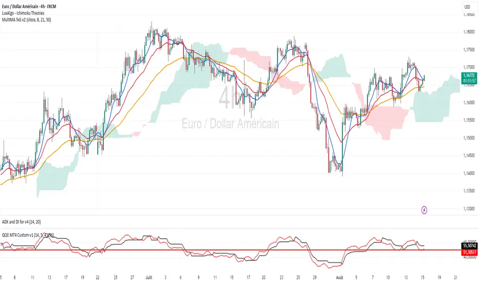
Simple Crossover MME 5/20
Description:
This indicator plots a 5-period Exponential Moving Average (EMA) in red and a 20-period EMA in blue.
It provides clear visual signals for crossovers:
A green triangle appears when the 5 EMA crosses above the 20 EMA (bullish signal).
A red triangle appears when the 5 EMA crosses below the 20 EMA (bearish signal).
Built-in alerts are available for both bullish and bearish crossover events.
Option 2 (More Detailed)
Title: 5 EMA / 20 EMA Crossover Strategy with Visual Signals & Alerts
Description:
This script is designed to track one of the most popular moving average strategies: the crossover between the 5-period and 20-period Exponential Moving Averages (EMA). It's a clean and straightforward tool for identifying potential shifts in short-term trend momentum.
Features:
5-Period EMA: Plotted in Red.
20-Period EMA: Plotted in Blue.
Bullish Crossover Signals: A green triangle is plotted below the price bar when the 5 EMA (Red) crosses above the 20 EMA (Blue), suggesting potential upward momentum.
Bearish Crossover Signals: A red triangle is plotted above the price bar when the 5 EMA (Red) crosses below the 20 EMA (Blue), suggesting potential downward momentum.
Customizable Alerts: The indicator includes built-in alert conditions. You can easily set up real-time notifications for every "buy" (crossover) or "sell" (crossunder) signal.
How to Use:
Add the indicator to your chart.
To receive notifications, create an alert and select this indicator as the condition. Choose either the "Bullish Crossover" or "Bearish Crossover" option.

SmartMind2The MACD (Moving Average Convergence Divergence) is a popular technical indicator in trading, primarily used to detect trends and possible reversal points.
How is the MACD structured?
The MACD indicator consists of three components:
MACD Line:
Calculated as the difference between two exponential moving averages (EMAs), commonly 12 and 26 periods.
Formula:
MACD Line
=
𝐸
𝑀
𝐴
12
(
Price
)
−
𝐸
𝑀
𝐴
26
(
Price
)
MACD Line=EMA
12
(Price)−EMA
26
(Price)
Signal Line:
An exponential moving average (usually 9 periods) of the MACD line.
Formula:
Signal Line
=
𝐸
𝑀
𝐴
9
(
MACD Line
)
Signal Line=EMA
9
(MACD Line)
Histogram:
Graphically represents the difference between the MACD line and the Signal line.
Formula:
Histogram
=
MACD Line
−
Signal Line
Histogram=MACD Line−Signal Line
Interpretation of MACD:
Buy Signal: Occurs when the MACD line crosses above the signal line (bullish signal).
Sell Signal: Occurs when the MACD line crosses below the signal line (bearish signal).
Trend Reversal: A divergence between price movements and the MACD indicates a potential reversal (e.g., rising prices with a falling MACD).
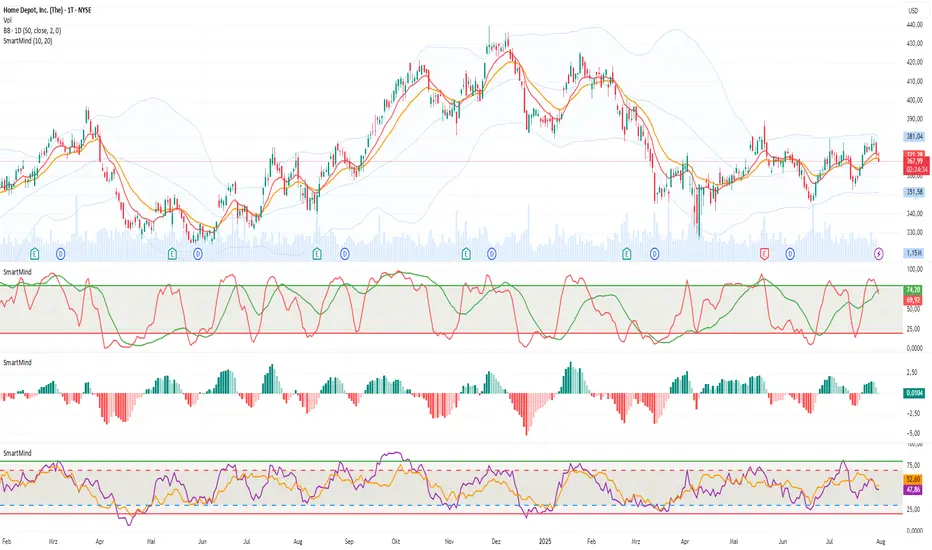
Volume MA Breakout T3 [Teyo69]🧭 Overview
Volume MA Breakout T3 highlights volume bars that exceed a dynamic moving average threshold. It helps traders visually identify volume breakouts—periods of significant buying or selling pressure—based on user-selected MA methods (SMA, EMA, DEMA).
🔍 Features
Volume Highlighting: Green bars indicate volume breakout above the MA; red bars otherwise.
Custom MA Options: Choose between SMA, EMA, or Double EMA for volume smoothing.
Dynamic Threshold: The moving average line adjusts based on user-defined length and method.
⚙️ Configuration
Length: Number of bars used for the moving average calculation (default: 14).
Method: Type of moving average to use:
"SMA" - Simple Moving Average
"EMA" - Exponential Moving Average
"Double EMA" - Double Exponential Moving Average
📈 How to Use
Apply to any chart to visualize volume behavior relative to its MA.
Look for green bars: These suggest volume is breaking out above its recent average—potential signal of momentum.
Red bars indicate normal/subdued volume.
⚠️ Limitations
Does not provide directional bias—use with price action or trend confirmation tools.
Works best with additional context (e.g., support/resistance, candle formations).
🧠 Advanced Tips
Use shorter MAs (e.g., 5–10) in volatile markets for more responsive signals.
Combine with OBV, MFI, or accumulation indicators for confluence.
📌 Notes
This is a volume-based filter, not a signal generator.
Useful for breakout traders and volume profile enthusiasts.
📜 Disclaimer
This script is for educational purposes only. Always test in a simulated environment before live trading. Not financial advice.
Price Volume Trend [sgbpulse]1. Introduction: What is Price Volume Trend (PVT)?
The Price Volume Trend (PVT) indicator is a powerful technical analysis tool designed to measure buying and selling pressure in the market based on price changes relative to trading volume. Unlike other indicators that focus solely on volume or price, PVT combines both components to provide a more comprehensive picture of trend strength.
How is it Calculated?
The PVT is calculated by adding or subtracting a proportional part of the daily volume from a cumulative total.
When the closing price rises, a proportional part of the daily volume (based on the percentage price change) is added to the previous PVT value.
When the closing price falls, a proportional part of the daily volume is subtracted from the previous PVT value.
If there is no change in price, the PVT value remains unchanged.
The result of this calculation is a cumulative line that rises when buying pressure is strong and falls when selling pressure dominates.
2. Why PVT? Comparison to Similar Indicators
While other indicators measure volume-price pressure, PVT offers a unique advantage:
PVT vs. On-Balance Volume (OBV):
OBV simply adds or subtracts the entire day's volume based on the closing direction (up/down), regardless of the magnitude of the price change. This means a 0.1% price change is treated the same as a 10% change.
PVT, on the other hand, gives proportional weight to volume based on the percentage price change. A trading day with a large price increase and high volume will impact the PVT significantly more than a small price increase with the same volume. This makes PVT more sensitive to trend strength and changes within it.
PVT vs. Accumulation/Distribution Line (A/D Line):
The A/D Line focuses on the relationship between the closing price and the bar's trading range (Close Location Value) and multiplies it by volume. It indicates whether the pressure is buying or selling within a single bar.
PVT focuses on the change between closing prices of consecutive bars, multiplying this by volume. It better reflects the flow of money into or out of an asset over time.
By combining volume with percentage price change, PVT provides deeper insights into trend confirmation, identifying divergences between price and volume, and spotting signs of weakness or strength in the current trend.
3. Indicator Settings (Inputs)
The "Price Volume Trend " indicator offers great flexibility for customization to your specific needs through the following settings:
Moving Average Type: Allows you to select the type of moving average used for the central line on the PVT. Your choice here will affect the line's responsiveness to PVT movements.
- "None" : No moving average will be displayed on the PVT.
- "SMA" (Simple Moving Average): A simple average, smoother, ideal for identifying longer-term trends in PVT.
- "SMA + Bollinger Bands": This unique option not only displays a Simple Moving Average but also activates the Bollinger Bands around the PVT. This is the recommended option for analyzing volatility and ranges using Bollinger Bands.
- "EMA" (Exponential Moving Average): An exponential average, giving more weight to recent data, responding faster to changes in PVT.
- "SMMA (RMA)" (Smoothed Moving Average): A smoothed average, providing extra smoothing, less sensitive to noise.
- "WMA" (Weighted Moving Average): A weighted average, giving progressively more weight to recent data, responding very quickly to changes in PVT.
Moving Average Length: Defines the number of bars used to calculate the moving average (and, if applicable, the standard deviation for the Bollinger Bands). A lower value will make the line more responsive, while a higher value will smooth it out.
PVT BB StdDev (Bollinger Bands Standard Deviation): Determines the width of the Bollinger Bands. A higher value will result in wider bands, making it less likely for the PVT to cross them. The standard value is 2.0.
4. Visual Aid: Current PVT Level Line
This indicator includes a unique and highly useful visual feature: a dynamic horizontal line displayed on the PVT graph.
Purpose: This line marks the exact level of the PVT on the most recent trading bar. It extends across the entire chart, allowing for a quick and intuitive comparison of the current level to past levels.
Why is it Important?
- Identifying Divergences: Often, an asset's price may be lower or higher than past levels, but the PVT level might be different. This auxiliary line makes it easy to spot situations where PVT is at a higher level when the price is lower, or vice-versa, which can signal potential trend changes (e.g., higher PVT than in the past while price is low could indicate strong accumulation).
- Quick Direction Indication: The line's color changes dynamically: it will be green if the PVT value on the last bar has increased (or remained the same) relative to the previous bar (indicating positive buying pressure), and red if the PVT value has decreased relative to the previous bar (indicating selling pressure). This provides an immediate visual cue about the direction of the cumulative momentum.
5. Important Note: Trading Risk
This indicator is intended for educational and informational purposes only and does not constitute investment advice or a recommendation for trading in any form whatsoever.
Trading in financial markets involves significant risk of capital loss. It is important to remember that past performance is not indicative of future results. All trading decisions are your sole responsibility. Never trade with money you cannot afford to lose.

Pullback Pro Dow Strategy v7 (ADX Filter)
### **Strategy Description (For TradingView)**
#### **Title:** Pullback Pro: Dow Theory & ADX Strategy
---
#### **1. Summary**
This strategy is designed to identify and trade pullbacks within an established trend, based on the core principles of Dow Theory. It uses market structure (pivot highs and lows) to determine the trend direction and an Exponential Moving Average (EMA) to pinpoint pullback entry opportunities.
To enhance trade quality and avoid ranging markets, an ADX (Average Directional Index) filter is integrated to ensure that entries are only taken when the trend has sufficient momentum.
---
#### **2. Core Logic: How It Works**
The strategy's logic is broken down into three main steps:
**Step 1: Trend Determination (Dow Theory)**
* The primary trend is identified by analyzing recent pivot points.
* An **Uptrend** is confirmed when the script detects a pattern of higher highs and higher lows (HH/HL).
* A **Downtrend** is confirmed by a pattern of lower highs and lower lows (LH/LL).
* If neither pattern is present, the strategy considers the market to be in a range and will not seek trades.
**Step 2: Entry Signal (Pullback to EMA)**
* Once a clear trend is established, the strategy waits for a price correction.
* **Long Entry:** In a confirmed uptrend, a long position is initiated when the price pulls back and crosses *under* the specified EMA.
* **Short Entry:** In a confirmed downtrend, a short position is initiated when the price rallies and crosses *over* the EMA.
**Step 3: Confirmation & Risk Management**
* **ADX Filter:** To ensure the trend is strong enough to trade, an entry signal is only validated if the ADX value is above a user-defined threshold (e.g., 25). This helps filter out weak signals during choppy or consolidating markets.
* **Stop Loss:** The initial Stop Loss is automatically and logically placed at the last market structure point:
* For long trades, it's placed at the `lastPivotLow`.
* For short trades, it's placed at the `lastPivotHigh`.
* **Take Profit:** Two Take Profit levels are calculated based on user-defined Risk-to-Reward (R:R) ratios. The strategy allows for partial profit-taking at the first target (TP1), moving the remainder of the position to the second target (TP2).
---
#### **3. Input Settings Explained**
**① Dow Theory Settings**
* **Pivot Lookback Period:** Determines the sensitivity for detecting pivot highs and lows. A smaller number makes it more sensitive to recent price swings; a larger number focuses on more significant, longer-term pivots.
**② Entry Logic (Pullback)**
* **Pullback EMA Length:** Sets the period for the Exponential Moving Average used to identify pullback entries.
**③ Risk & Exit Management**
* **Take Profit 1 R:R:** Sets the Risk-to-Reward ratio for the first take-profit target.
* **Take Profit 1 (%):** The percentage of the position to be closed when TP1 is hit.
* **Take Profit 2 R:R:** Sets the Risk-to-Reward ratio for the final take-profit target.
**④ Filters**
* **Use ADX Trend Filter:** A master switch to enable or disable the ADX filter.
* **ADX Length:** The lookback period for the ADX calculation.
* **ADX Threshold:** The minimum ADX value required to confirm a trade signal. Trades will only be placed if the ADX is above this level.
---
#### **4. Best Practices & Recommendations**
* This is a trend-following system. It is designed to perform best in markets that exhibit clear, sustained trending behavior.
* It may underperform in choppy, sideways, or strongly ranging markets. The ADX filter is designed to help mitigate this, but no filter is perfect.
* **Crucially, you must backtest this strategy thoroughly** on your preferred financial instrument and timeframe before considering any live application.
* Experiment with the `Pivot Lookback Period`, `Pullback EMA Length`, and `ADX Threshold` to optimize performance for a specific market's characteristics.
---
#### **DISCLAIMER**
This script is provided for educational and informational purposes only. It does not constitute financial advice. All trading involves a high level of risk, and past performance is not indicative of future results. You are solely responsible for your own trading decisions. The author assumes no liability for any financial losses you may incur from using this strategy. Always conduct your own research and due diligence.
Dynamic Ray BandsAbout Dynamic Ray Bands
Dynamic Ray Bands is a volatility-adaptive envelope indicator that adjusts in real time to evolving market conditions. It uses a Double Exponential Moving Average (DEMA) as its central trend reference, with upper and lower bands scaled according to current volatility measured by the Average True Range (ATR).
This creates a dynamic structure that visually frames price action, helping traders identify areas of potential trend continuation, overextension, or mean reversion.
How It Works
🟡 Centerline (DEMA)
The central yellow line is a Double Exponential Moving Average, which offers a smoother, less laggy trend signal than traditional moving averages. It represents the market’s short- to medium-term “equilibrium.”
🔵 Outer Bands
Plotted at:
Upper Band = DEMA + (ATR × outerMultiplier)
Lower Band = DEMA - (ATR × outerMultiplier)
These bands define the extreme bounds of current volatility. When price breaks above or below them, it can signal strong directional momentum or overbought/oversold conditions, depending on context. They're often used as trend breakout zones or to time exits after extended runs.
🟣 Inner Bands
Plotted closer to the DEMA:
Inner Upper = DEMA + (ATR × innerMultiplier)
Inner Lower = DEMA - (ATR × innerMultiplier)
These are preliminary volatility thresholds, offering early cues for potential expansion or reversal. They may be used for scalping, tight stop zones, or pre-breakout positioning.
🔁 Dynamic Width (Bands are Dynamically Adjusted Per Tick)
The width of both inner and outer bands is based on ATR (Average True Range), which is recalculated in real time. This means:
During high volatility, the bands expand, allowing for wider price fluctuations.
During low volatility, the bands contract, tightening range expectations.
Unlike fixed-width channels or standard Bollinger Bands (which use standard deviation), this per-tick adjustment via ATR enables Dynamic Ray Bands to reduce false signals in choppy markets and remain more reactive during trending conditions.
⚙️ Inputs
DMA Length — Period for the central DEMA.
ATR Length — Lookback used for ATR volatility calculations.
Outer Band Multiplier — Controls sensitivity of extreme bands.
Inner Band Multiplier — Controls proximity of inner bands.
Show Inner Bands — Toggle for plotting the inner zone.
🔔 Alerts
Alert conditions are included for:
Price closing above/below the outer bands (trend momentum or overextension)
Price closing above/below the inner bands (early signs of strength/weakness)
🧭 Use Cases
Breakout detection — Catch price continuation beyond the outer bands.
Volatility filtering — Adjust trade logic based on band width.
Mean reversion — Monitor for snapbacks toward the DEMA after price stretches too far.
Trend guidance — Use band slope and price position to confirm direction.
⚠️ Disclaimer
This script is intended for educational and informational purposes only. It does not constitute financial advice or a recommendation to trade any specific market or security. Always test indicators thoroughly before using them in live trading.
Trend Tracker ProTrend Tracker Pro - Advanced Trend Following Indicator
Overview
Trend Tracker Pro is a sophisticated trend-following indicator that combines the power of Exponential Moving Average (EMA) and Average True Range (ATR) to identify market trends and generate precise buy/sell signals. This indicator is designed to help traders capture trending moves while filtering out market noise.
🎯 Key Features
✅ Dynamic Trend Detection
Uses EMA and ATR-based bands to identify trend direction
Automatically adjusts to market volatility
Clear visual trend line that changes color based on market direction
✅ Precise Signal Generation
Buy signals when trend changes to bullish
Sell signals when trend changes to bearish
Reduces false signals by requiring actual trend changes
✅ Visual Clarity
Green trend line: Bullish trend
Red trend line: Bearish trend
Gray trend line: Sideways/neutral trend
Triangle arrows for buy/sell signals
Clear BUY/SELL text labels
✅ Customizable Settings
Trend Length: Adjustable period for EMA and ATR calculation (default: 14)
ATR Multiplier: Controls sensitivity of trend bands (default: 2.0)
Show/Hide Signals: Toggle signal arrows on/off
Show/Hide Labels: Toggle text labels on/off
✅ Built-in Information Panel
Real-time trend direction display
Current trend level value
ATR value for volatility reference
Last signal information
✅ TradingView Alerts
Buy signal alerts
Sell signal alerts
Customizable alert messages
🔧 How It Works
Algorithm Logic:
1.
Calculate EMA: Uses exponential moving average for trend baseline
2.
Calculate ATR: Measures market volatility
3.
Create Bands: Upper band = EMA + (ATR × Multiplier), Lower band = EMA - (ATR × Multiplier)
4.
Determine Trend:
Price above upper band → Bullish trend (trend line = lower band)
Price below lower band → Bearish trend (trend line = upper band)
Price between bands → Continue previous trend
5.
Generate Signals: Signal occurs when trend direction changes
📊 Best Use Cases
✅ Trending Markets
Excellent for capturing strong directional moves
Works well in both bull and bear markets
Ideal for swing trading and position trading
✅ Multiple Timeframes
Effective on all timeframes from 15 minutes to daily
Higher timeframes provide more reliable signals
Can be used for both scalping and long-term investing
✅ Various Asset Classes
Stocks, Forex, Cryptocurrencies, Commodities
Particularly effective in volatile markets
Adapts automatically to different volatility levels
⚙️ Recommended Settings
Conservative Trading (Lower Risk)
Trend Length: 20
ATR Multiplier: 2.5
Best for: Long-term positions, lower frequency signals
Balanced Trading (Default)
Trend Length: 14
ATR Multiplier: 2.0
Best for: Swing trading, moderate frequency signals
Aggressive Trading (Higher Risk)
Trend Length: 10
ATR Multiplier: 1.5
Best for: Day trading, higher frequency signals
🎨 Visual Elements
Trend Line: Main indicator line that follows the trend
Signal Arrows: Triangle shapes indicating buy/sell points
Text Labels: Clear "BUY" and "SELL" text markers
Information Table: Real-time status panel in top-right corner
Color Coding: Intuitive green/red color scheme
⚠️ Important Notes
Risk Management
Always use proper position sizing
Set stop-losses based on ATR values
Consider market conditions and volatility
Not recommended for ranging/sideways markets
Signal Confirmation
Consider using with other indicators for confirmation
Pay attention to volume and market structure
Be aware of major news events and market sessions
Backtesting Recommended
Test the indicator on historical data
Optimize parameters for your specific trading style
Consider transaction costs in your analysis
Logarithmic Moving Average (LMA) [QuantAlgo]🟢 Overview
The Logarithmic Moving Average (LMA) uses advanced logarithmic weighting to create a dynamic trend-following indicator that prioritizes recent price action while maintaining statistical significance. Unlike traditional moving averages that use linear or exponential weights, this indicator employs logarithmic decay functions to create a more sophisticated price averaging system that adapts to market volatility and momentum conditions.
The indicator displays a smoothed signal line that oscillates around zero, with positive values indicating bullish momentum and negative values indicating bearish momentum. The signal incorporates trend quality assessment, momentum confirmation, and multiple filtering mechanisms to help traders and investors identify trend continuation and reversal opportunities across different timeframes and asset classes.
🟢 How It Works
The indicator's core innovation lies in its logarithmic weighting system, where weights are calculated using the formula: w = 1.0 / math.pow(math.log(i + steepness), 2) The steepness parameter controls how aggressively recent data is prioritized over historical data, creating a dynamic weight decay that can be fine-tuned for different trading styles. This logarithmic approach provides more nuanced weight distribution compared to exponential moving averages, offering better responsiveness while maintaining stability.
The LMA calculation combines multiple sophisticated components. First, it calculates the logarithmic weighted average of closing prices. Then it measures the slope of this average over a 10-period lookback: lmaSlope = (lma - lma ) / lma * 100 The system also incorporates trend quality assessment using R-squared correlation analysis of log-transformed prices, measuring how well the price data fits a linear trend model over the specified period.
The final signal generation uses the formula: signal = lmaSlope * (0.5 + rSquared * 0.5) which combines the LMA slope with trend quality weighting. When momentum confirmation is enabled, the indicator calculates annualized log-return momentum and applies a multiplier when the momentum direction aligns with the signal direction, strengthening confirmed signals while filtering out weak or counter-trend movements.
🟢 How to Use
1. Signal Interpretation and Threshold Zones
Positive Values (Above Zero): LMA slope indicating bullish momentum with upward price trajectory relative to logarithmic baseline
Negative Values (Below Zero): LMA slope indicating bearish momentum with downward price trajectory relative to logarithmic baseline
Zero Line Crosses: Signal transitions between bullish and bearish regimes, indicating potential trend changes
Long Entry Threshold Zone: Area above positive threshold (default 0.5) indicating confirmed bullish signals suitable for long positions
Short Entry Threshold Zone: Area below negative threshold (default -0.5) indicating confirmed bearish signals suitable for short positions
Extreme Values: Signals exceeding ±1.0 represent strong momentum conditions with higher probability of continuation
2. Momentum Confirmation and Visual Analysis
Signal Color Intensity: Gradient coloring shows signal strength, with brighter colors indicating stronger momentum
Bar Coloring: Optional price bar coloring matches signal direction for quick visual trend identification
Position Labels: Real-time position classification (Bullish/Bearish/Neutral) displayed on the latest bar
Momentum Weight Factor: When short-term log-return momentum aligns with LMA signal direction, the signal receives additional weight confirmation
Trend Quality Component: R-squared values weight the signal strength, with higher correlation indicating more reliable trend conditions
3. Examples: Preconfigured Settings
Default: Universally applicable configuration balanced for medium-term investing and general trading across multiple timeframes and asset classes.
Scalping: Highly responsive setup with shorter period and higher steepness for ultra-short-term trades on 1-15 minute charts, optimized for quick momentum shifts.
Swing Trading: Extended period with moderate steepness and increased smoothing for multi-day positions, designed to filter noise while capturing larger price swings on 1-4 hour and daily charts.
Trend Following: Maximum smoothing with lower steepness for established trend identification, generating fewer but more reliable signals optimal for daily and weekly timeframes.
Mean Reversion: Shorter period with high steepness for counter-trend strategies, more sensitive to extreme moves and reversal opportunities in ranging market conditions.
Custom EMA High/Low & SMA - [GSK-VIZAG-AP-INDIA] Custom EMA High/Low & SMA -
1. Overview
This indicator overlays a dynamic combination of Exponential Moving Averages (EMA) and Simple Moving Average (SMA) to identify momentum shifts and potential entry/exit zones. It highlights bullish or bearish conditions using color-coded SMA logic and provides visual Buy/Sell signals based on smart crossover and state-based logic.
2. Purpose / Use Case
Designed for traders who want to visually identify momentum breakouts, trend reversals, or pullback opportunities, this tool helps:
Spot high-probability buy/sell zones
Confirm price strength relative to volatility bands (EMA High/Low)
Time entries based on clean visual cues
It works well in trend-following strategies, particularly in intraday or swing setups across any liquid market (indices, stocks, crypto, etc.).
3. Key Features & Logic
✅ EMA High/Low Channel: Acts as dynamic support/resistance boundaries using 20-period EMAs on high and low prices.
✅ Timeframe-Specific SMA: A 33-period SMA calculated from a user-defined timeframe (default: 10-minute) for flexible multi-timeframe analysis.
✅ Signal Generation:
Buy: When SMA drops below EMA Low and close is above EMA High.
Sell: When SMA rises above EMA High and price closes below both EMAs.
Optionally, signals also fire based on SMA color changes (green = bullish, red = bearish).
✅ Strict or Loose Signal Logic: Choose between precise crossovers or broader state-based conditions.
✅ Debugging Tools: Optional markers for granular insight into condition logic.
4. User Inputs & Settings
Input Description
EMA High Length Period for EMA of high prices (default: 20)
EMA Low Length Period for EMA of low prices (default: 20)
SMA Length Period for Simple Moving Average (default: 33)
SMA Timeframe Timeframe for SMA (default: “10”)
Show Buy/Sell Arrows Enable visual arrow signals for Buy/Sell
Strict Signal Logic ON = crossover-based signals; OFF = state logic
Plot Signals on SMA Color Change Enable signals on SMA color shifts (Green/Red)
Show Debug Markers Plot small markers to debug condition logic
5. Visual Elements Explained
🔵 EMA High Line – Blue line marking dynamic resistance
🔴 EMA Low Line – Red line marking dynamic support
🟡 SMA Line – Color-coded based on position:
Green if SMA < EMA Low (Bullish)
Red if SMA > EMA High (Bearish)
Yellow otherwise (Neutral)
✅ BUY / SELL Labels – Displayed below or above candles on valid signals
🛠️ Debug Circles/Triangles – Help visually understand the signal logic when enabled
6. Usage Tips
Best used on 5–30 min timeframes for intraday setups or 1H+ for swing trades.
Confirm signals with volume, price action, or other confluences (like support/resistance).
Use strict mode for more accurate entries, and non-strict mode for broader trend views.
Ideal for identifying pullbacks into trend, or early reversals after volatility squeezes.
7. What Makes It Unique
Multi-timeframe SMA integrated with EMA High/Low bands
Dual signal logic (crossover + color shift)
Visually intuitive and beginner-friendly
Minimal clutter with dynamic signal labeling
Debug mode for transparency and learning
8. Alerts & Automation
The indicator includes built-in alert conditions for:
📈 Buy Alert: Triggered when a bullish condition is detected.
🔻 Sell Alert: Triggered when bearish confirmation is detected.
These alerts can be used with TradingView's alert system for real-time notifications or bot integrations.
9. Technical Concepts Used
EMA (Exponential Moving Average): Reacts faster to recent price, ideal for trend channels
SMA (Simple Moving Average): Smoother average for detecting general trend direction
Crossover Logic: Checks when SMA crosses over or under EMA levels
Color Coding: Visual signal enhancement based on relative positioning
Multi-Timeframe Analysis: SMA calculated on a custom timeframe, powerful for confirmation
10. Disclaimer
This script is for educational and informational purposes only. It is not financial advice. Always backtest thoroughly and validate on demo accounts before applying to live markets. Trading involves risk, and past performance does not guarantee future results.
11. Author Signature
📌 Indicator Name: Custom EMA High/Low & SMA -
👤 Author: GSK-VIZAG-AP-INDIA