Multi SMA'sRepublished: The original script violated house rules by including an external link to Backtest Rookies.
Background
This is a simple “multi” SMA indicator so that multiple SMA’s can be monitored whilst only using a single indicator slot. It also has a couple of features that let you mix time frames and de-clutter the chart.
The code is open for anyone to modify and a copy
About the Indicator
Although the indicator does nothing more than it says on the tin, There are a couple of points worth mentioning:
The indicator will let you view up to 4 SMA’s
You can set the period for each SMA independently
You can set the resolution for each SMA independently (So you can see the see the daily SMA level when on the 15-minute chart for example)
Each SMA can be turned on/off independently to avoid clutter.
Screenshot - Default Settings
"backtest"に関するスクリプトを検索

Backtest Strategy Optimizer Adapter - Supertrend ExampleSample Code
This is a sample code for my Backtest Strategy Optimizer Adapter library.
You can find the library at:
Backtest Strategy Optimizer Tester
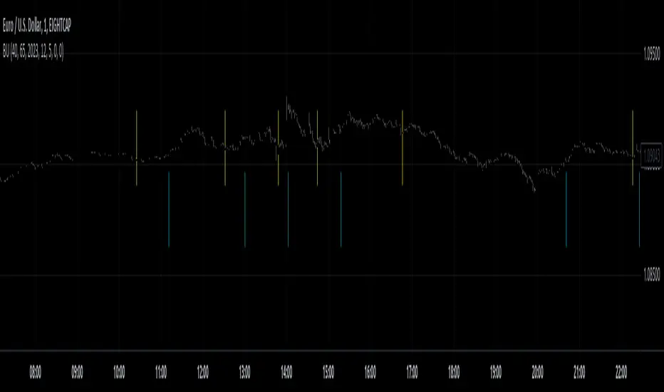
With this indicator, you will be able to run one or multiple backtests with different variables (combinations). For example, you can run dozens of backtests of Supertrend at once with an increment factor of 0.1, or whatever you prefer. This way, you can easily grab the most profitable settings and use them in your strategy. The chart above shows different color plots, each indicating a profit backtest equal to tradingview backtesting system. This code uses my backtest library, available in my profile.
Below the code you should edit yourself
You can use ChatGPT or write a python script to autogenerate code for you.
// #################################################################
// # ENTRIES AND EXITS
// #################################################################
// You can use the link and code in the description to create
// your code for the desired number of entries / exits.
// #################################################################
// AUTO GENERATED CODE
// ▼▼▼▼▼▼▼▼▼▼▼▼▼▼▼▼▼▼▼▼▼▼▼▼▼▼▼▼▼▼▼▼▼▼▼▼▼▼▼▼▼▼▼▼▼▼▼▼▼▼▼▼▼▼▼▼▼▼▼▼▼▼▼▼▼
= ti.supertrend(10, 0.1)
= ti.supertrend(10, 0.2)
= ti.supertrend(10, 0.3)
= ti.supertrend(10, 0.4)
// 005 etc...
pnl_001 = backtest.profit(date_start, date_end, entry_001, exit_001)
pnl_002 = backtest.profit(date_start, date_end, entry_002, exit_002)
pnl_003 = backtest.profit(date_start, date_end, entry_003, exit_003)
pnl_004 = backtest.profit(date_start, date_end, entry_004, exit_004)
plot(pnl_001, title='0.1', color=backtest.color(001))
plot(pnl_002, title='0.2', color=backtest.color(002))
plot(pnl_003, title='0.3', color=backtest.color(003))
plot(pnl_004, title='0.4', color=backtest.color(004))
// Make sure you set the correct array size.
// The amount of tests + 1 (e.g. 4 tests you set it to 5)
var results_list = array.new_string(5)
if (ta.change(pnl_001))
array.set(results_list, 0, str.tostring(pnl_001) + '|0.1')
if (ta.change(pnl_002))
array.set(results_list, 1, str.tostring(pnl_002) + '|0.2')
if (ta.change(pnl_003))
array.set(results_list, 2, str.tostring(pnl_003) + '|0.3')
if (ta.change(pnl_004))
array.set(results_list, 3, str.tostring(pnl_004) + '|0.4')
// ▲▲▲▲▲▲▲▲▲▲▲▲▲▲▲▲▲▲▲▲▲▲▲▲▲▲▲▲▲▲▲▲▲▲▲▲▲▲▲▲▲▲▲▲▲▲▲▲▲▲▲▲▲▲▲▲▲▲▲▲▲▲▲▲▲
// AUTO GENERATED CODE
// #################################################################
QFL single TF with alertsBacktesting compatible QFL pine script w/alerts
This version of QFL was made based on this one:
From author:
www.tradingview.com
I made the following additions according to my requirements:
- I need to use pine script 4
- I needed to avoid repainting issues so I'm not calling directly security, I'm using the wrapper function.
- There might be still repainting issues when you use "max base age" which uses the function "barssince" so be careful, you can disable it by setting its value to zero.
- Alerts so I can use it for automated trading and bots
- In order to make this signal compatible with the backtest script there's an option provided in the settings. If you enable this option this indicator will plot 1 whenever there's a BUY signal. This will allow the backtest to pick the "QFL Buy" from external indicator so it can perform the backtest.
I recommend some of these settings to start playing with the chart in 15 min / QFL in 1, 2 or 4 hours.
The higher the TF the more conservative.
QFL with 3.5% is pretty popular but you can try higher QFL percentage settings for a more conservative approach.

Backtester UtilityLook ahead bias is the most evil bias responsible for overestimation of the performance of the trading system.
As the Bar replay feature is only available to paid users which is a great tool for manual testing of the trading system. Leaving other users prone to the evil of Look ahead bias.
So that I have developed this indicator which will help users to manually backtest the strategies.
This indicator hides the price action after specified date and time.
Here are the steps for using the indicator.
1) Hide your chart manually.
2) Plot the indicator.
3) Change the input of time and date after which you want to hide price action.
4) Change the script according to your trading strategy.
5) Enjoy the free of cost manual backtesting.
Good trading buddies !
Note : This post is only for educational purpose , it does not contain any financial advise.
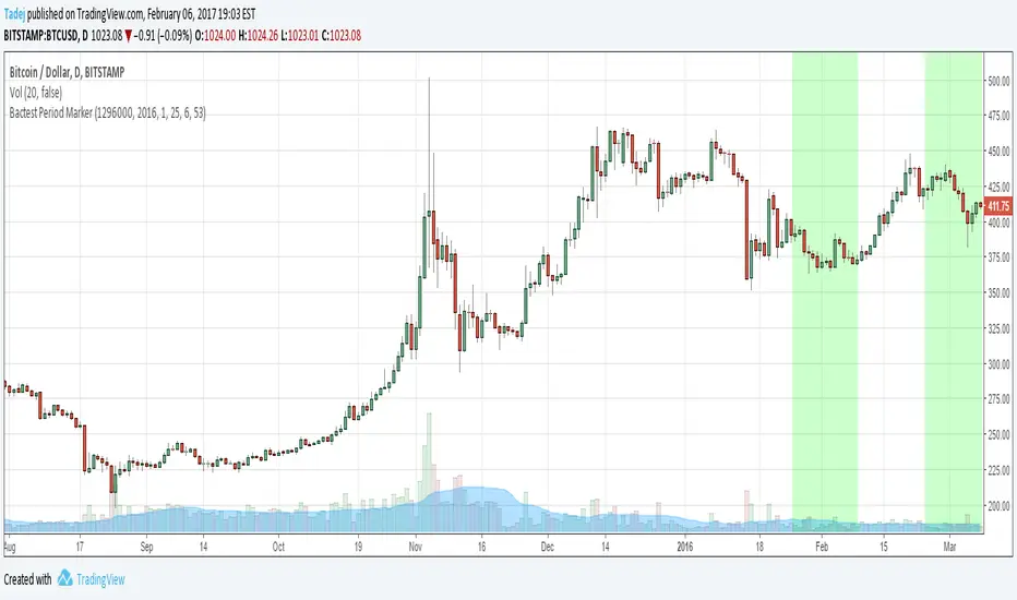
Bactest Period MarkerSimple script that will mark backtest periods (if you have to run backtests in multiple parts, like on CryptoTrader )
Backtest optimized Smoothed Log-Space MACD [elindicador.ai]This indicator is backtest-optimized for the Daily Timeframe. Usage is straight forward as showed in the chart. Once the histogram flips to blue it signals a good change of an uptrend. If it flips to orange this suggests a likely downtrend. If you use this Indicator on the $TOTAL chart it will also show reliable buy/sell signals with a little dot.

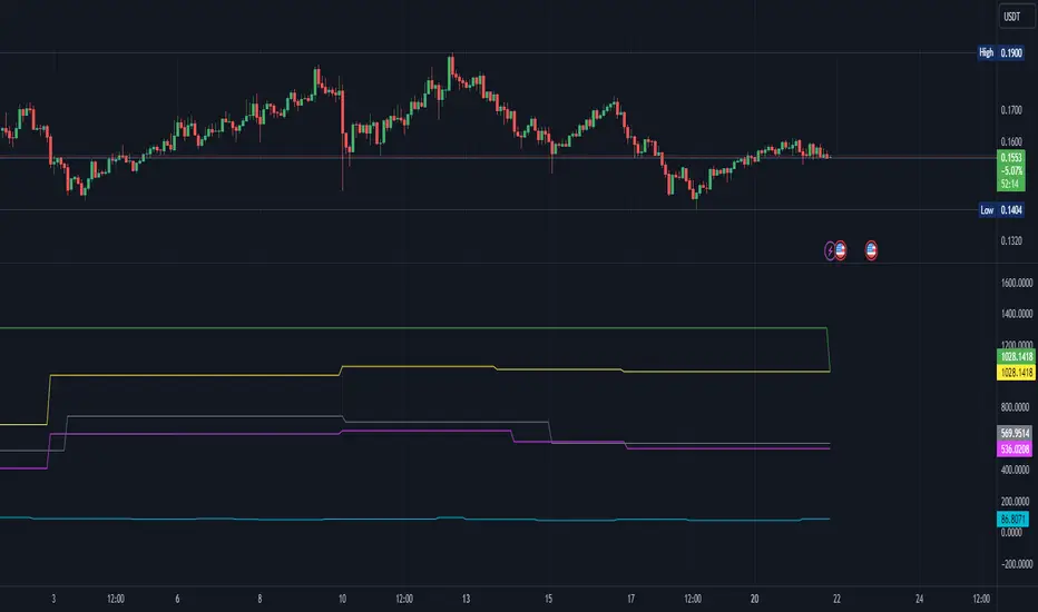
GKD-M Baseline Optimizer [Loxx]Giga Kaleidoscope GKD-M Baseline Optimizer is a Metamorphosis module included in Loxx's "Giga Kaleidoscope Modularized Trading System".
The Baseline Optimizer enables traders to backtest over 60 moving averages using variable period inputs. It then exports the baseline with the highest cumulative win rate per candle to any baseline-enabled GKD backtest. To perform the backtesting, the trader selects an initial period input (default is 60) and a skip value that increments the initial period input up to seven times. For instance, if a skip value of 5 is chosen, the Baseline Optimizer will run the backtest for the selected moving average on periods such as 60, 65, 70, 75, and so on, up to 90. If the user selects an initial period input of 45 and a skip value of 2, the Baseline Optimizer will conduct backtests for the chosen moving average on periods like 45, 47, 49, 51, and so forth, up to 57.
The Baseline Optimizer provides a table displaying the output of the backtests for a specified date range. The table output represents the cumulative win rate for the given date range.
On the Metamorphosis side of the Baseline Optimizer, a cumulative backtest is calculated for each candle within the date range. This means that each candle may exhibit a different distribution of period inputs with the highest win rate for a particular moving average. The Baseline Optimizer identifies the period input combination with the highest win rates for long and short positions and creates a win-rate adaptive long and short moving average chart. The moving average used for shorts differs from the moving average used for longs, and the moving average for each candle may vary from any other candle. This customized baseline can then be exported to all baseline-enabled GKD backtests.
The backtest employed in the Baseline Optimizer is a Solo Confirmation Simple, allowing only one take profit and one stop loss to be set.
Lastly, the Baseline Optimizer incorporates Goldie Locks Zone filtering, which can be utilized for signal generation in advanced GKD backtests.
█ Moving Averages included in the Baseline Optimizer
Adaptive Moving Average - AMA
ADXvma - Average Directional Volatility Moving Average
Ahrens Moving Average
Alexander Moving Average - ALXMA
Deviation Scaled Moving Average - DSMA
Donchian
Double Exponential Moving Average - DEMA
Double Smoothed Exponential Moving Average - DSEMA
Double Smoothed FEMA - DSFEMA
Double Smoothed Range Weighted EMA - DSRWEMA
Double Smoothed Wilders EMA - DSWEMA
Double Weighted Moving Average - DWMA
Exponential Moving Average - EMA
Fast Exponential Moving Average - FEMA
Fractal Adaptive Moving Average - FRAMA
Generalized DEMA - GDEMA
Generalized Double DEMA - GDDEMA
Hull Moving Average (Type 1) - HMA1
Hull Moving Average (Type 2) - HMA2
Hull Moving Average (Type 3) - HMA3
Hull Moving Average (Type 4) - HMA4
IE /2 - Early T3 by Tim Tilson
Integral of Linear Regression Slope - ILRS
Kaufman Adaptive Moving Average - KAMA
Leader Exponential Moving Average
Linear Regression Value - LSMA ( Least Squares Moving Average )
Linear Weighted Moving Average - LWMA
McGinley Dynamic
McNicholl EMA
Non-Lag Moving Average
Ocean NMA Moving Average - ONMAMA
One More Moving Average - OMA
Parabolic Weighted Moving Average
Probability Density Function Moving Average - PDFMA
Quadratic Regression Moving Average - QRMA
Regularized EMA - REMA
Range Weighted EMA - RWEMA
Recursive Moving Trendline
Simple Decycler - SDEC
Simple Jurik Moving Average - SJMA
Simple Moving Average - SMA
Sine Weighted Moving Average
Smoothed LWMA - SLWMA
Smoothed Moving Average - SMMA
Smoother
Super Smoother
T3
Three-pole Ehlers Butterworth
Three-pole Ehlers Smoother
Triangular Moving Average - TMA
Triple Exponential Moving Average - TEMA
Two-pole Ehlers Butterworth
Two-pole Ehlers smoother
Variable Index Dynamic Average - VIDYA
Variable Moving Average - VMA
Volume Weighted EMA - VEMA
Volume Weighted Moving Average - VWMA
Zero-Lag DEMA - Zero Lag Exponential Moving Average
Zero-Lag Moving Average
Zero Lag TEMA - Zero Lag Triple Exponential Moving Average
Adaptive Moving Average - AMA
The Adaptive Moving Average (AMA) is a moving average that changes its sensitivity to price moves depending on the calculated volatility. It becomes more sensitive during periods when the price is moving smoothly in a certain direction and becomes less sensitive when the price is volatile.
ADXvma - Average Directional Volatility Moving Average
Linnsoft's ADXvma formula is a volatility-based moving average, with the volatility being determined by the value of the ADX indicator.
The ADXvma has the SMA in Chande's CMO replaced with an EMA , it then uses a few more layers of EMA smoothing before the "Volatility Index" is calculated.
A side effect is, those additional layers slow down the ADXvma when you compare it to Chande's Variable Index Dynamic Average VIDYA .
The ADXVMA provides support during uptrends and resistance during downtrends and will stay flat for longer, but will create some of the most accurate market signals when it decides to move.
Ahrens Moving Average
Richard D. Ahrens's Moving Average promises "Smoother Data" that isn't influenced by the occasional price spike. It works by using the Open and the Close in his formula so that the only time the Ahrens Moving Average will change is when the candlestick is either making new highs or new lows.
Alexander Moving Average - ALXMA
This Moving Average uses an elaborate smoothing formula and utilizes a 7 period Moving Average. It corresponds to fitting a second-order polynomial to seven consecutive observations. This moving average is rarely used in trading but is interesting as this Moving Average has been applied to diffusion indexes that tend to be very volatile.
Deviation Scaled Moving Average - DSMA
The Deviation-Scaled Moving Average is a data smoothing technique that acts like an exponential moving average with a dynamic smoothing coefficient. The smoothing coefficient is automatically updated based on the magnitude of price changes. In the Deviation-Scaled Moving Average, the standard deviation from the mean is chosen to be the measure of this magnitude. The resulting indicator provides substantial smoothing of the data even when price changes are small while quickly adapting to these changes.
Donchian
Donchian Channels are three lines generated by moving average calculations that comprise an indicator formed by upper and lower bands around a midrange or median band. The upper band marks the highest price of a security over N periods while the lower band marks the lowest price of a security over N periods.
Double Exponential Moving Average - DEMA
The Double Exponential Moving Average ( DEMA ) combines a smoothed EMA and a single EMA to provide a low-lag indicator. It's primary purpose is to reduce the amount of "lagging entry" opportunities, and like all Moving Averages, the DEMA confirms uptrends whenever price crosses on top of it and closes above it, and confirms downtrends when the price crosses under it and closes below it - but with significantly less lag.
Double Smoothed Exponential Moving Average - DSEMA
The Double Smoothed Exponential Moving Average is a lot less laggy compared to a traditional EMA . It's also considered a leading indicator compared to the EMA , and is best utilized whenever smoothness and speed of reaction to market changes are required.
Double Smoothed FEMA - DSFEMA
Same as the Double Exponential Moving Average (DEMA), but uses a faster version of EMA for its calculation.
Double Smoothed Range Weighted EMA - DSRWEMA
Range weighted exponential moving average (EMA) is, unlike the "regular" range weighted average calculated in a different way. Even though the basis - the range weighting - is the same, the way how it is calculated is completely different. By definition this type of EMA is calculated as a ratio of EMA of price*weight / EMA of weight. And the results are very different and the two should be considered as completely different types of averages. The higher than EMA to price changes responsiveness when the ranges increase remains in this EMA too and in those cases this EMA is clearly leading the "regular" EMA. This version includes double smoothing.
Double Smoothed Wilders EMA - DSWEMA
Welles Wilder was frequently using one "special" case of EMA (Exponential Moving Average) that is due to that fact (that he used it) sometimes called Wilder's EMA. This version is adding double smoothing to Wilder's EMA in order to make it "faster" (it is more responsive to market prices than the original) and is still keeping very smooth values.
Double Weighted Moving Average - DWMA
Double weighted moving average is an LWMA (Linear Weighted Moving Average). Instead of doing one cycle for calculating the LWMA, the indicator is made to cycle the loop 2 times. That produces a smoother values than the original LWMA
Exponential Moving Average - EMA
The EMA places more significance on recent data points and moves closer to price than the SMA ( Simple Moving Average ). It reacts faster to volatility due to its emphasis on recent data and is known for its ability to give greater weight to recent and more relevant data. The EMA is therefore seen as an enhancement over the SMA .
Fast Exponential Moving Average - FEMA
An Exponential Moving Average with a short look-back period.
Fractal Adaptive Moving Average - FRAMA
The Fractal Adaptive Moving Average by John Ehlers is an intelligent adaptive Moving Average which takes the importance of price changes into account and follows price closely enough to display significant moves whilst remaining flat if price ranges. The FRAMA does this by dynamically adjusting the look-back period based on the market's fractal geometry.
Generalized DEMA - GDEMA
The double exponential moving average (DEMA), was developed by Patrick Mulloy in an attempt to reduce the amount of lag time found in traditional moving averages. It was first introduced in the February 1994 issue of the magazine Technical Analysis of Stocks & Commodities in Mulloy's article "Smoothing Data with Faster Moving Averages.". Instead of using fixed multiplication factor in the final DEMA formula, the generalized version allows you to change it. By varying the "volume factor" form 0 to 1 you apply different multiplications and thus producing DEMA with different "speed" - the higher the volume factor is the "faster" the DEMA will be (but also the slope of it will be less smooth). The volume factor is limited in the calculation to 1 since any volume factor that is larger than 1 is increasing the overshooting to the extent that some volume factors usage makes the indicator unusable.
Generalized Double DEMA - GDDEMA
The double exponential moving average (DEMA), was developed by Patrick Mulloy in an attempt to reduce the amount of lag time found in traditional moving averages. It was first introduced in the February 1994 issue of the magazine Technical Analysis of Stocks & Commodities in Mulloy's article "Smoothing Data with Faster Moving Averages''. This is an extension of the Generalized DEMA using Tim Tillsons (the inventor of T3) idea, and is using GDEMA of GDEMA for calculation (which is the "middle step" of T3 calculation). Since there are no versions showing that middle step, this version covers that too. The result is smoother than Generalized DEMA, but is less smooth than T3 - one has to do some experimenting in order to find the optimal way to use it, but in any case, since it is "faster" than the T3 (Tim Tillson T3) and still smooth, it looks like a good compromise between speed and smoothness.
Hull Moving Average (Type 1) - HMA1
Alan Hull's HMA makes use of weighted moving averages to prioritize recent values and greatly reduce lag whilst maintaining the smoothness of a traditional Moving Average. For this reason, it's seen as a well-suited Moving Average for identifying entry points. This version uses SMA for smoothing.
Hull Moving Average (Type 2) - HMA2
Alan Hull's HMA makes use of weighted moving averages to prioritize recent values and greatly reduce lag whilst maintaining the smoothness of a traditional Moving Average. For this reason, it's seen as a well-suited Moving Average for identifying entry points. This version uses EMA for smoothing.
Hull Moving Average (Type 3) - HMA3
Alan Hull's HMA makes use of weighted moving averages to prioritize recent values and greatly reduce lag whilst maintaining the smoothness of a traditional Moving Average. For this reason, it's seen as a well-suited Moving Average for identifying entry points. This version uses LWMA for smoothing.
Hull Moving Average (Type 4) - HMA4
Alan Hull's HMA makes use of weighted moving averages to prioritize recent values and greatly reduce lag whilst maintaining the smoothness of a traditional Moving Average. For this reason, it's seen as a well-suited Moving Average for identifying entry points. This version uses SMMA for smoothing.
IE /2 - Early T3 by Tim Tilson and T3 new
The T3 moving average is a type of technical indicator used in financial analysis to identify trends in price movements. It is similar to the Exponential Moving Average (EMA) and the Double Exponential Moving Average (DEMA), but uses a different smoothing algorithm.
The T3 moving average is calculated using a series of exponential moving averages that are designed to filter out noise and smooth the data. The resulting smoothed data is then weighted with a non-linear function to produce a final output that is more responsive to changes in trend direction.
The T3 moving average can be customized by adjusting the length of the moving average, as well as the weighting function used to smooth the data. It is commonly used in conjunction with other technical indicators as part of a larger trading strategy.
Integral of Linear Regression Slope - ILRS
A Moving Average where the slope of a linear regression line is simply integrated as it is fitted in a moving window of length N (natural numbers in maths) across the data. The derivative of ILRS is the linear regression slope. ILRS is not the same as a SMA ( Simple Moving Average ) of length N, which is actually the midpoint of the linear regression line as it moves across the data.
Kaufman Adaptive Moving Average - KAMA
Developed by Perry Kaufman, Kaufman's Adaptive Moving Average (KAMA) is a moving average designed to account for market noise or volatility. KAMA will closely follow prices when the price swings are relatively small and the noise is low.
Leader Exponential Moving Average
The Leader EMA was created by Giorgos E. Siligardos who created a Moving Average which was able to eliminate lag altogether whilst maintaining some smoothness. It was first described during his research paper "MACD Leader" where he applied this to the MACD to improve its signals and remove its lagging issue. This filter uses his leading MACD's "modified EMA" and can be used as a zero lag filter.
Linear Regression Value - LSMA ( Least Squares Moving Average )
LSMA as a Moving Average is based on plotting the end point of the linear regression line. It compares the current value to the prior value and a determination is made of a possible trend, eg. the linear regression line is pointing up or down.
Linear Weighted Moving Average - LWMA
LWMA reacts to price quicker than the SMA and EMA . Although it's similar to the Simple Moving Average , the difference is that a weight coefficient is multiplied to the price which means the most recent price has the highest weighting, and each prior price has progressively less weight. The weights drop in a linear fashion.
McGinley Dynamic
John McGinley created this Moving Average to track prices better than traditional Moving Averages. It does this by incorporating an automatic adjustment factor into its formula, which speeds (or slows) the indicator in trending, or ranging, markets.
McNicholl EMA
Dennis McNicholl developed this Moving Average to use as his center line for his "Better Bollinger Bands" indicator and was successful because it responded better to volatility changes over the standard SMA and managed to avoid common whipsaws.
Non-lag moving average
The Non Lag Moving average follows price closely and gives very quick signals as well as early signals of price change. As a standalone Moving Average, it should not be used on its own, but as an additional confluence tool for early signals.
Ocean NMA Moving Average - ONMAMA
Created by Jim Sloman, the NMA is a moving average that automatically adjusts to volatility without being programmed to do so. For more info, read his guide "Ocean Theory, an Introduction"
One More Moving Average (OMA)
The One More Moving Average (OMA) is a technical indicator that calculates a series of Jurik-style moving averages in order to reduce noise and provide smoother price data. It uses six exponential moving averages to generate the final value, with the length of the moving averages determined by an adaptive algorithm that adjusts to the current market conditions. The algorithm calculates the average period by comparing the signal to noise ratio and using this value to determine the length of the moving averages. The resulting values are used to generate the final value of the OMA, which can be used to identify trends and potential changes in trend direction.
Parabolic Weighted Moving Average
The Parabolic Weighted Moving Average is a variation of the Linear Weighted Moving Average . The Linear Weighted Moving Average calculates the average by assigning different weights to each element in its calculation. The Parabolic Weighted Moving Average is a variation that allows weights to be changed to form a parabolic curve. It is done simply by using the Power parameter of this indicator.
Probability Density Function Moving Average - PDFMA
Probability density function based MA is a sort of weighted moving average that uses probability density function to calculate the weights. By its nature it is similar to a lot of digital filters.
Quadratic Regression Moving Average - QRMA
A quadratic regression is the process of finding the equation of the parabola that best fits a set of data. This moving average is an obscure concept that was posted to Forex forums in around 2008.
Regularized EMA - REMA
The regularized exponential moving average (REMA) by Chris Satchwell is a variation on the EMA (see Exponential Moving Average) designed to be smoother but not introduce too much extra lag.
Range Weighted EMA - RWEMA
This indicator is a variation of the range weighted EMA. The variation comes from a possible need to make that indicator a bit less "noisy" when it comes to slope changes. The method used for calculating this variation is the method described by Lee Leibfarth in his article "Trading With An Adaptive Price Zone".
Recursive Moving Trendline
Dennis Meyers's Recursive Moving Trendline uses a recursive (repeated application of a rule) polynomial fit, a technique that uses a small number of past values estimations of price and today's price to predict tomorrow's price.
Simple Decycler - SDEC
The Ehlers Simple Decycler study is a virtually zero-lag technical indicator proposed by John F. Ehlers. The original idea behind this study (and several others created by John F. Ehlers) is that market data can be considered a continuum of cycle periods with different cycle amplitudes. Thus, trending periods can be considered segments of longer cycles, or, in other words, low-frequency segments. Applying the right filter might help identify these segments.
Simple Loxx Moving Average - SLMA
A three stage moving average combining an adaptive EMA, a Kalman Filter, and a Kauffman adaptive filter.
Simple Moving Average - SMA
The SMA calculates the average of a range of prices by adding recent prices and then dividing that figure by the number of time periods in the calculation average. It is the most basic Moving Average which is seen as a reliable tool for starting off with Moving Average studies. As reliable as it may be, the basic moving average will work better when it's enhanced into an EMA .
Sine Weighted Moving Average
The Sine Weighted Moving Average assigns the most weight at the middle of the data set. It does this by weighting from the first half of a Sine Wave Cycle and the most weighting is given to the data in the middle of that data set. The Sine WMA closely resembles the TMA (Triangular Moving Average).
Smoothed LWMA - SLWMA
A smoothed version of the LWMA
Smoothed Moving Average - SMMA
The Smoothed Moving Average is similar to the Simple Moving Average ( SMA ), but aims to reduce noise rather than reduce lag. SMMA takes all prices into account and uses a long lookback period. Due to this, it's seen as an accurate yet laggy Moving Average.
Smoother
The Smoother filter is a faster-reacting smoothing technique which generates considerably less lag than the SMMA ( Smoothed Moving Average ). It gives earlier signals but can also create false signals due to its earlier reactions. This filter is sometimes wrongly mistaken for the superior Jurik Smoothing algorithm.
Super Smoother
The Super Smoother filter uses John Ehlers’s “Super Smoother” which consists of a Two pole Butterworth filter combined with a 2-bar SMA ( Simple Moving Average ) that suppresses the 22050 Hz Nyquist frequency: A characteristic of a sampler, which converts a continuous function or signal into a discrete sequence.
Three-pole Ehlers Butterworth
The 3 pole Ehlers Butterworth (as well as the Two pole Butterworth) are both superior alternatives to the EMA and SMA . They aim at producing less lag whilst maintaining accuracy. The 2 pole filter will give you a better approximation for price, whereas the 3 pole filter has superior smoothing.
Three-pole Ehlers smoother
The 3 pole Ehlers smoother works almost as close to price as the above mentioned 3 Pole Ehlers Butterworth. It acts as a strong baseline for signals but removes some noise. Side by side, it hardly differs from the Three Pole Ehlers Butterworth but when examined closely, it has better overshoot reduction compared to the 3 pole Ehlers Butterworth.
Triangular Moving Average - TMA
The TMA is similar to the EMA but uses a different weighting scheme. Exponential and weighted Moving Averages will assign weight to the most recent price data. Simple moving averages will assign the weight equally across all the price data. With a TMA (Triangular Moving Average), it is double smoother (averaged twice) so the majority of the weight is assigned to the middle portion of the data.
Triple Exponential Moving Average - TEMA
The TEMA uses multiple EMA calculations as well as subtracting lag to create a tool which can be used for scalping pullbacks. As it follows price closely, its signals are considered very noisy and should only be used in extremely fast-paced trading conditions.
Two-pole Ehlers Butterworth
The 2 pole Ehlers Butterworth (as well as the three pole Butterworth mentioned above) is another filter that cuts out the noise and follows the price closely. The 2 pole is seen as a faster, leading filter over the 3 pole and follows price a bit more closely. Analysts will utilize both a 2 pole and a 3 pole Butterworth on the same chart using the same period, but having both on chart allows its crosses to be traded.
Two-pole Ehlers smoother
A smoother version of the Two pole Ehlers Butterworth. This filter is the faster version out of the 3 pole Ehlers Butterworth. It does a decent job at cutting out market noise whilst emphasizing a closer following to price over the 3 pole Ehlers .
Variable Index Dynamic Average - VIDYA
Variable Index Dynamic Average Technical Indicator ( VIDYA ) was developed by Tushar Chande. It is an original method of calculating the Exponential Moving Average ( EMA ) with the dynamically changing period of averaging.
Variable Moving Average - VMA
The Variable Moving Average (VMA) is a study that uses an Exponential Moving Average being able to automatically adjust its smoothing factor according to the market volatility.
Volume Weighted EMA - VEMA
An EMA that uses a volume and price weighted calculation instead of the standard price input.
Volume Weighted Moving Average - VWMA
A Volume Weighted Moving Average is a moving average where more weight is given to bars with heavy volume than with light volume. Thus the value of the moving average will be closer to where most trading actually happened than it otherwise would be without being volume weighted.
Zero-Lag DEMA - Zero Lag Double Exponential Moving Average
John Ehlers's Zero Lag DEMA's aim is to eliminate the inherent lag associated with all trend following indicators which average a price over time. Because this is a Double Exponential Moving Average with Zero Lag, it has a tendency to overshoot and create a lot of false signals for swing trading. It can however be used for quick scalping or as a secondary indicator for confluence.
Zero-Lag Moving Average
The Zero Lag Moving Average is described by its creator, John Ehlers , as a Moving Average with absolutely no delay. And it's for this reason that this filter will cause a lot of abrupt signals which will not be ideal for medium to long-term traders. This filter is designed to follow price as close as possible whilst de-lagging data instead of basing it on regular data. The way this is done is by attempting to remove the cumulative effect of the Moving Average.
Zero-Lag TEMA - Zero Lag Triple Exponential Moving Average
Just like the Zero Lag DEMA , this filter will give you the fastest signals out of all the Zero Lag Moving Averages. This is useful for scalping but dangerous for medium to long-term traders, especially during market Volatility and news events. Having no lag, this filter also has no smoothing in its signals and can cause some very bizarre behavior when applied to certain indicators.
█ Volatility Goldie Locks Zone
The Goldie Locks Zone volatility filter is the standard first-pass filter used in all advanced GKD backtests (Complex, Super Complex, and Full GKd). This filter requires the price to fall within a range determined by multiples of volatility. The Goldie Locks Zone is separate from the core Baseline and utilizes its own moving average with Loxx's Exotic Source Types you can read about below.
On the chart, you will find green and red dots positioned at the top, indicating whether a candle qualifies for a long or short trade respectively. Additionally, green and red triangles are located at the bottom of the chart, signifying whether the trigger has crossed up or down and qualifies within the Goldie Locks zone. The Goldie Locks zone is represented by a white color on the mean line, indicating low volatility levels that are not suitable for trading.
█ Volatility Types Included in the Baseline Optimizer
The GKD system utilizes volatility-based take profits and stop losses. Each take profit and stop loss is calculated as a multiple of volatility. Users can also adjust the multiplier values in the settings.
This module includes 17 types of volatility:
Close-to-Close
Parkinson
Garman-Klass
Rogers-Satchell
Yang-Zhang
Garman-Klass-Yang-Zhang
Exponential Weighted Moving Average
Standard Deviation of Log Returns
Pseudo GARCH(2,2)
Average True Range
True Range Double
Standard Deviation
Adaptive Deviation
Median Absolute Deviation
Efficiency-Ratio Adaptive ATR
Mean Absolute Deviation
Static Percent
Various volatility estimators and indicators that investors and traders can use to measure the dispersion or volatility of a financial instrument's price. Each estimator has its strengths and weaknesses, and the choice of estimator should depend on the specific needs and circumstances of the user.
Close-to-Close
Close-to-Close volatility is a classic and widely used volatility measure, sometimes referred to as historical volatility.
Volatility is an indicator of the speed of a stock price change. A stock with high volatility is one where the price changes rapidly and with a larger amplitude. The more volatile a stock is, the riskier it is.
Close-to-close historical volatility is calculated using only a stock's closing prices. It is the simplest volatility estimator. However, in many cases, it is not precise enough. Stock prices could jump significantly during a trading session and return to the opening value at the end. That means that a considerable amount of price information is not taken into account by close-to-close volatility.
Despite its drawbacks, Close-to-Close volatility is still useful in cases where the instrument doesn't have intraday prices. For example, mutual funds calculate their net asset values daily or weekly, and thus their prices are not suitable for more sophisticated volatility estimators.
Parkinson
Parkinson volatility is a volatility measure that uses the stock’s high and low price of the day.
The main difference between regular volatility and Parkinson volatility is that the latter uses high and low prices for a day, rather than only the closing price. This is useful as close-to-close prices could show little difference while large price movements could have occurred during the day. Thus, Parkinson's volatility is considered more precise and requires less data for calculation than close-to-close volatility.
One drawback of this estimator is that it doesn't take into account price movements after the market closes. Hence, it systematically undervalues volatility. This drawback is addressed in the Garman-Klass volatility estimator.
Garman-Klass
Garman-Klass is a volatility estimator that incorporates open, low, high, and close prices of a security.
Garman-Klass volatility extends Parkinson's volatility by taking into account the opening and closing prices. As markets are most active during the opening and closing of a trading session, it makes volatility estimation more accurate.
Garman and Klass also assumed that the process of price change follows a continuous diffusion process (Geometric Brownian motion). However, this assumption has several drawbacks. The method is not robust for opening jumps in price and trend movements.
Despite its drawbacks, the Garman-Klass estimator is still more effective than the basic formula since it takes into account not only the price at the beginning and end of the time interval but also intraday price extremes.
Researchers Rogers and Satchell have proposed a more efficient method for assessing historical volatility that takes into account price trends. See Rogers-Satchell Volatility for more detail.
Rogers-Satchell
Rogers-Satchell is an estimator for measuring the volatility of securities with an average return not equal to zero.
Unlike Parkinson and Garman-Klass estimators, Rogers-Satchell incorporates a drift term (mean return not equal to zero). As a result, it provides better volatility estimation when the underlying is trending.
The main disadvantage of this method is that it does not take into account price movements between trading sessions. This leads to an underestimation of volatility since price jumps periodically occur in the market precisely at the moments between sessions.
A more comprehensive estimator that also considers the gaps between sessions was developed based on the Rogers-Satchel formula in the 2000s by Yang-Zhang. See Yang Zhang Volatility for more detail.
Yang-Zhang
Yang Zhang is a historical volatility estimator that handles both opening jumps and the drift and has a minimum estimation error.
Yang-Zhang volatility can be thought of as a combination of the overnight (close-to-open volatility) and a weighted average of the Rogers-Satchell volatility and the day’s open-to-close volatility. It is considered to be 14 times more efficient than the close-to-close estimator.
Garman-Klass-Yang-Zhang
Garman-Klass-Yang-Zhang (GKYZ) volatility estimator incorporates the returns of open, high, low, and closing prices in its calculation.
GKYZ volatility estimator takes into account overnight jumps but not the trend, i.e., it assumes that the underlying asset follows a Geometric Brownian Motion (GBM) process with zero drift. Therefore, the GKYZ volatility estimator tends to overestimate the volatility when the drift is different from zero. However, for a GBM process, this estimator is eight times more efficient than the close-to-close volatility estimator.
Exponential Weighted Moving Average
The Exponentially Weighted Moving Average (EWMA) is a quantitative or statistical measure used to model or describe a time series. The EWMA is widely used in finance, with the main applications being technical analysis and volatility modeling.
The moving average is designed such that older observations are given lower weights. The weights decrease exponentially as the data point gets older – hence the name exponentially weighted.
The only decision a user of the EWMA must make is the parameter lambda. The parameter decides how important the current observation is in the calculation of the EWMA. The higher the value of lambda, the more closely the EWMA tracks the original time series.
Standard Deviation of Log Returns
This is the simplest calculation of volatility. It's the standard deviation of ln(close/close(1)).
Pseudo GARCH(2,2)
This is calculated using a short- and long-run mean of variance multiplied by ?.
?avg(var;M) + (1 ? ?) avg(var;N) = 2?var/(M+1-(M-1)L) + 2(1-?)var/(M+1-(M-1)L)
Solving for ? can be done by minimizing the mean squared error of estimation; that is, regressing L^-1var - avg(var; N) against avg(var; M) - avg(var; N) and using the resulting beta estimate as ?.
Average True Range
The average true range (ATR) is a technical analysis indicator, introduced by market technician J. Welles Wilder Jr. in his book New Concepts in Technical Trading Systems, that measures market volatility by decomposing the entire range of an asset price for that period.
The true range indicator is taken as the greatest of the following: current high less the current low; the absolute value of the current high less the previous close; and the absolute value of the current low less the previous close. The ATR is then a moving average, generally using 14 days, of the true ranges.
True Range Double
A special case of ATR that attempts to correct for volatility skew.
Standard Deviation
Standard deviation is a statistic that measures the dispersion of a dataset relative to its mean and is calculated as the square root of the variance. The standard deviation is calculated as the square root of variance by determining each data point's deviation relative to the mean. If the data points are further from the mean, there is a higher deviation within the data set; thus, the more spread out the data, the higher the standard deviation.
Adaptive Deviation
By definition, the Standard Deviation (STD, also represented by the Greek letter sigma ? or the Latin letter s) is a measure that is used to quantify the amount of variation or dispersion of a set of data values. In technical analysis, we usually use it to measure the level of current volatility.
Standard Deviation is based on Simple Moving Average calculation for mean value. This version of standard deviation uses the properties of EMA to calculate what can be called a new type of deviation, and since it is based on EMA, we can call it EMA deviation. Additionally, Perry Kaufman's efficiency ratio is used to make it adaptive (since all EMA type calculations are nearly perfect for adapting).
The difference when compared to the standard is significant--not just because of EMA usage, but the efficiency ratio makes it a "bit more logical" in very volatile market conditions.
Median Absolute Deviation
The median absolute deviation is a measure of statistical dispersion. Moreover, the MAD is a robust statistic, being more resilient to outliers in a data set than the standard deviation. In the standard deviation, the distances from the mean are squared, so large deviations are weighted more heavily, and thus outliers can heavily influence it. In the MAD, the deviations of a small number of outliers are irrelevant.
Because the MAD is a more robust estimator of scale than the sample variance or standard deviation, it works better with distributions without a mean or variance, such as the Cauchy distribution.
For this indicator, a manual recreation of the quantile function in Pine Script is used. This is so users have a full inside view into how this is calculated.
Efficiency-Ratio Adaptive ATR
Average True Range (ATR) is a widely used indicator for many occasions in technical analysis. It is calculated as the RMA of the true range. This version adds a "twist": it uses Perry Kaufman's Efficiency Ratio to calculate adaptive true range.
Mean Absolute Deviation
The mean absolute deviation (MAD) is a measure of variability that indicates the average distance between observations and their mean. MAD uses the original units of the data, which simplifies interpretation. Larger values signify that the data points spread out further from the average. Conversely, lower values correspond to data points bunching closer to it. The mean absolute deviation is also known as the mean deviation and average absolute deviation.
This definition of the mean absolute deviation sounds similar to the standard deviation (SD). While both measure variability, they have different calculations. In recent years, some proponents of MAD have suggested that it replace the SD as the primary measure because it is a simpler concept that better fits real life.
█ Loxx's Expanded Source Types Included in Baseline Optimizer
This indicator allows you to select from 33 source types. They are as follows:
Close
Open
High
Low
Median
Typical
Weighted
Average
Average Median Body
Trend Biased
Trend Biased (Extreme)
HA Close
HA Open
HA High
HA Low
HA Median
HA Typical
HA Weighted
HA Average
HA Average Median Body
HA Trend Biased
HA Trend Biased (Extreme)
HAB Close
HAB Open
HAB High
HAB Low
HAB Median
HAB Typical
HAB Weighted
HAB Average
HAB Average Median Body
HAB Trend Biased
HAB Trend Biased (Extreme)
What are Heiken Ashi "better" candles?
Heiken Ashi "better" candles are a modified version of the standard Heiken Ashi candles, which are a popular charting technique used in technical analysis. Heiken Ashi candles help traders identify trends and potential reversal points by smoothing out price data and reducing market noise. The "better formula" was proposed by Sebastian Schmidt in an article published by BNP Paribas in Warrants & Zertifikate, a German magazine, in August 2004. The aim of this formula is to further improve the smoothing of the Heiken Ashi chart and enhance its effectiveness in identifying trends and reversals.
Standard Heiken Ashi candles are calculated using the following formulas:
Heiken Ashi Close = (Open + High + Low + Close) / 4
Heiken Ashi Open = (Previous Heiken Ashi Open + Previous Heiken Ashi Close) / 2
Heiken Ashi High = Max (High, Heiken Ashi Open, Heiken Ashi Close)
Heiken Ashi Low = Min (Low, Heiken Ashi Open, Heiken Ashi Close)
The "better formula" modifies the standard Heiken Ashi calculation by incorporating additional smoothing, which can help reduce noise and make it easier to identify trends and reversals. The modified formulas for Heiken Ashi "better" candles are as follows:
Better Heiken Ashi Close = (Open + High + Low + Close) / 4
Better Heiken Ashi Open = (Previous Better Heiken Ashi Open + Previous Better Heiken Ashi Close) / 2
Better Heiken Ashi High = Max (High, Better Heiken Ashi Open, Better Heiken Ashi Close)
Better Heiken Ashi Low = Min (Low, Better Heiken Ashi Open, Better Heiken Ashi Close)
Smoothing Factor = 2 / (N + 1), where N is the chosen period for smoothing
Smoothed Better Heiken Ashi Open = (Better Heiken Ashi Open * Smoothing Factor) + (Previous Smoothed Better Heiken Ashi Open * (1 - Smoothing Factor))
Smoothed Better Heiken Ashi Close = (Better Heiken Ashi Close * Smoothing Factor) + (Previous Smoothed Better Heiken Ashi Close * (1 - Smoothing Factor))
The smoothed Better Heiken Ashi Open and Close values are then used to calculate the smoothed Better Heiken Ashi High and Low values, resulting in "better" candles that provide a clearer representation of the market trend and potential reversal points.
Heiken Ashi "better" candles, as mentioned previously, provide a clearer representation of market trends and potential reversal points by reducing noise and smoothing out price data. When using these candles in conjunction with other technical analysis tools and indicators, traders can gain valuable insights into market behavior and make more informed decisions.
To effectively use Heiken Ashi "better" candles in your trading strategy, consider the following tips:
-Trend Identification: Heiken Ashi "better" candles can help you identify the prevailing trend in the market. When the majority of the candles are green (or another color, depending on your chart settings) and there are no or few lower wicks, it may indicate a strong uptrend. Conversely, when the majority of the candles are red (or another color) and there are no or few upper wicks, it may signal a strong downtrend.
-Trend Reversals: Look for potential trend reversals when a change in the color of the candles occurs, especially when accompanied by longer wicks. For example, if a green candle with a long lower wick is followed by a red candle, it could indicate a bearish reversal. Similarly, a red candle with a long upper wick followed by a green candle may suggest a bullish reversal.
-Support and Resistance: You can use Heiken Ashi "better" candles to identify potential support and resistance levels. When the candles are consistently moving in one direction and then suddenly change color with longer wicks, it could indicate the presence of a support or resistance level.
-Stop-Loss and Take-Profit: Using Heiken Ashi "better" candles can help you manage risk by determining optimal stop-loss and take-profit levels. For instance, you can place your stop-loss below the low of the most recent green candle in an uptrend or above the high of the most recent red candle in a downtrend.
-Confirming Signals: Heiken Ashi "better" candles should be used in conjunction with other technical indicators, such as moving averages, oscillators, or chart patterns, to confirm signals and improve the accuracy of your analysis.
In this implementation, you have the choice of AMA, KAMA, or T3 smoothing. These are as follows:
Kaufman Adaptive Moving Average (KAMA)
The Kaufman Adaptive Moving Average (KAMA) is a type of adaptive moving average used in technical analysis to smooth out price fluctuations and identify trends. The KAMA adjusts its smoothing factor based on the market's volatility, making it more responsive in volatile markets and smoother in calm markets. The KAMA is calculated using three different efficiency ratios that determine the appropriate smoothing factor for the current market conditions. These ratios are based on the noise level of the market, the speed at which the market is moving, and the length of the moving average. The KAMA is a popular choice among traders who prefer to use adaptive indicators to identify trends and potential reversals.
Adaptive Moving Average
The Adaptive Moving Average (AMA) is a type of moving average that adjusts its sensitivity to price movements based on market conditions. It uses a ratio between the current price and the highest and lowest prices over a certain lookback period to determine its level of smoothing. The AMA can help reduce lag and increase responsiveness to changes in trend direction, making it useful for traders who want to follow trends while avoiding false signals. The AMA is calculated by multiplying a smoothing constant with the difference between the current price and the previous AMA value, then adding the result to the previous AMA value.
T3
The T3 moving average is a type of technical indicator used in financial analysis to identify trends in price movements. It is similar to the Exponential Moving Average (EMA) and the Double Exponential Moving Average (DEMA), but uses a different smoothing algorithm.
The T3 moving average is calculated using a series of exponential moving averages that are designed to filter out noise and smooth the data. The resulting smoothed data is then weighted with a non-linear function to produce a final output that is more responsive to changes in trend direction.
The T3 moving average can be customized by adjusting the length of the moving average, as well as the weighting function used to smooth the data. It is commonly used in conjunction with other technical indicators as part of a larger trading strategy.
█ Giga Kaleidoscope Modularized Trading System
Core components of an NNFX algorithmic trading strategy
The NNFX algorithm is built on the principles of trend, momentum, and volatility. There are six core components in the NNFX trading algorithm:
1. Volatility - price volatility; e.g., Average True Range, True Range Double, Close-to-Close, etc.
2. Baseline - a moving average to identify price trend
3. Confirmation 1 - a technical indicator used to identify trends
4. Confirmation 2 - a technical indicator used to identify trends
5. Continuation - a technical indicator used to identify trends
6. Volatility/Volume - a technical indicator used to identify volatility/volume breakouts/breakdown
7. Exit - a technical indicator used to determine when a trend is exhausted
8. Metamorphosis - a technical indicator that produces a compound signal from the combination of other GKD indicators*
*(not part of the NNFX algorithm)
What is Volatility in the NNFX trading system?
In the NNFX (No Nonsense Forex) trading system, ATR (Average True Range) is typically used to measure the volatility of an asset. It is used as a part of the system to help determine the appropriate stop loss and take profit levels for a trade. ATR is calculated by taking the average of the true range values over a specified period.
True range is calculated as the maximum of the following values:
-Current high minus the current low
-Absolute value of the current high minus the previous close
-Absolute value of the current low minus the previous close
ATR is a dynamic indicator that changes with changes in volatility. As volatility increases, the value of ATR increases, and as volatility decreases, the value of ATR decreases. By using ATR in NNFX system, traders can adjust their stop loss and take profit levels according to the volatility of the asset being traded. This helps to ensure that the trade is given enough room to move, while also minimizing potential losses.
Other types of volatility include True Range Double (TRD), Close-to-Close, and Garman-Klass
What is a Baseline indicator?
The baseline is essentially a moving average, and is used to determine the overall direction of the market.
The baseline in the NNFX system is used to filter out trades that are not in line with the long-term trend of the market. The baseline is plotted on the chart along with other indicators, such as the Moving Average (MA), the Relative Strength Index (RSI), and the Average True Range (ATR).
Trades are only taken when the price is in the same direction as the baseline. For example, if the baseline is sloping upwards, only long trades are taken, and if the baseline is sloping downwards, only short trades are taken. This approach helps to ensure that trades are in line with the overall trend of the market, and reduces the risk of entering trades that are likely to fail.
By using a baseline in the NNFX system, traders can have a clear reference point for determining the overall trend of the market, and can make more informed trading decisions. The baseline helps to filter out noise and false signals, and ensures that trades are taken in the direction of the long-term trend.
What is a Confirmation indicator?
Confirmation indicators are technical indicators that are used to confirm the signals generated by primary indicators. Primary indicators are the core indicators used in the NNFX system, such as the Average True Range (ATR), the Moving Average (MA), and the Relative Strength Index (RSI).
The purpose of the confirmation indicators is to reduce false signals and improve the accuracy of the trading system. They are designed to confirm the signals generated by the primary indicators by providing additional information about the strength and direction of the trend.
Some examples of confirmation indicators that may be used in the NNFX system include the Bollinger Bands, the MACD (Moving Average Convergence Divergence), and the MACD Oscillator. These indicators can provide information about the volatility, momentum, and trend strength of the market, and can be used to confirm the signals generated by the primary indicators.
In the NNFX system, confirmation indicators are used in combination with primary indicators and other filters to create a trading system that is robust and reliable. By using multiple indicators to confirm trading signals, the system aims to reduce the risk of false signals and improve the overall profitability of the trades.
What is a Continuation indicator?
In the NNFX (No Nonsense Forex) trading system, a continuation indicator is a technical indicator that is used to confirm a current trend and predict that the trend is likely to continue in the same direction. A continuation indicator is typically used in conjunction with other indicators in the system, such as a baseline indicator, to provide a comprehensive trading strategy.
What is a Volatility/Volume indicator?
Volume indicators, such as the On Balance Volume (OBV), the Chaikin Money Flow (CMF), or the Volume Price Trend (VPT), are used to measure the amount of buying and selling activity in a market. They are based on the trading volume of the market, and can provide information about the strength of the trend. In the NNFX system, volume indicators are used to confirm trading signals generated by the Moving Average and the Relative Strength Index. Volatility indicators include Average Direction Index, Waddah Attar, and Volatility Ratio. In the NNFX trading system, volatility is a proxy for volume and vice versa.
By using volume indicators as confirmation tools, the NNFX trading system aims to reduce the risk of false signals and improve the overall profitability of trades. These indicators can provide additional information about the market that is not captured by the primary indicators, and can help traders to make more informed trading decisions. In addition, volume indicators can be used to identify potential changes in market trends and to confirm the strength of price movements.
What is an Exit indicator?
The exit indicator is used in conjunction with other indicators in the system, such as the Moving Average (MA), the Relative Strength Index (RSI), and the Average True Range (ATR), to provide a comprehensive trading strategy.
The exit indicator in the NNFX system can be any technical indicator that is deemed effective at identifying optimal exit points. Examples of exit indicators that are commonly used include the Parabolic SAR, the Average Directional Index (ADX), and the Chandelier Exit.
The purpose of the exit indicator is to identify when a trend is likely to reverse or when the market conditions have changed, signaling the need to exit a trade. By using an exit indicator, traders can manage their risk and prevent significant losses.
In the NNFX system, the exit indicator is used in conjunction with a stop loss and a take profit order to maximize profits and minimize losses. The stop loss order is used to limit the amount of loss that can be incurred if the trade goes against the trader, while the take profit order is used to lock in profits when the trade is moving in the trader's favor.
Overall, the use of an exit indicator in the NNFX trading system is an important component of a comprehensive trading strategy. It allows traders to manage their risk effectively and improve the profitability of their trades by exiting at the right time.
What is an Metamorphosis indicator?
The concept of a metamorphosis indicator involves the integration of two or more GKD indicators to generate a compound signal. This is achieved by evaluating the accuracy of each indicator and selecting the signal from the indicator with the highest accuracy. As an illustration, let's consider a scenario where we calculate the accuracy of 10 indicators and choose the signal from the indicator that demonstrates the highest accuracy.
The resulting output from the metamorphosis indicator can then be utilized in a GKD-BT backtest by occupying a slot that aligns with the purpose of the metamorphosis indicator. The slot can be a GKD-B, GKD-C, or GKD-E slot, depending on the specific requirements and objectives of the indicator. This allows for seamless integration and utilization of the compound signal within the GKD-BT framework.
How does Loxx's GKD (Giga Kaleidoscope Modularized Trading System) implement the NNFX algorithm outlined above?
Loxx's GKD v2.0 system has five types of modules (indicators/strategies). These modules are:
1. GKD-BT - Backtesting module (Volatility, Number 1 in the NNFX algorithm)
2. GKD-B - Baseline module (Baseline and Volatility/Volume, Numbers 1 and 2 in the NNFX algorithm)
3. GKD-C - Confirmation 1/2 and Continuation module (Confirmation 1/2 and Continuation, Numbers 3, 4, and 5 in the NNFX algorithm)
4. GKD-V - Volatility/Volume module (Confirmation 1/2, Number 6 in the NNFX algorithm)
5. GKD-E - Exit module (Exit, Number 7 in the NNFX algorithm)
6. GKD-M - Metamorphosis module (Metamorphosis, Number 8 in the NNFX algorithm, but not part of the NNFX algorithm)
(additional module types will added in future releases)
Each module interacts with every module by passing data to A backtest module wherein the various components of the GKD system are combined to create a trading signal.
That is, the Baseline indicator passes its data to Volatility/Volume. The Volatility/Volume indicator passes its values to the Confirmation 1 indicator. The Confirmation 1 indicator passes its values to the Confirmation 2 indicator. The Confirmation 2 indicator passes its values to the Continuation indicator. The Continuation indicator passes its values to the Exit indicator, and finally, the Exit indicator passes its values to the Backtest strategy.
This chaining of indicators requires that each module conform to Loxx's GKD protocol, therefore allowing for the testing of every possible combination of technical indicators that make up the six components of the NNFX algorithm.
What does the application of the GKD trading system look like?
Example trading system:
Backtest: Full GKD Backtest
Baseline: Hull Moving Average
Volatility/Volume: Hurst Exponent
Confirmation 1: Kase Peak Oscillator
Confirmation 2: uf2018
Continuation: Vortex
Exit: Rex Oscillator
Metamorphosis: Baseline Optimizer as shown on the chart above
Each GKD indicator is denoted with a module identifier of either: GKD-BT, GKD-B, GKD-C, GKD-V, GKD-M, or GKD-E. This allows traders to understand to which module each indicator belongs and where each indicator fits into the GKD system.
█ Giga Kaleidoscope Modularized Trading System Signals
Standard Entry
1. GKD-C Confirmation gives signal
2. Baseline agrees
3. Price inside Goldie Locks Zone Minimum
4. Price inside Goldie Locks Zone Maximum
5. Confirmation 2 agrees
6. Volatility/Volume agrees
1-Candle Standard Entry
1a. GKD-C Confirmation gives signal
2a. Baseline agrees
3a. Price inside Goldie Locks Zone Minimum
4a. Price inside Goldie Locks Zone Maximum
Next Candle
1b. Price retraced
2b. Baseline agrees
3b. Confirmation 1 agrees
4b. Confirmation 2 agrees
5b. Volatility/Volume agrees
Baseline Entry
1. GKD-B Basline gives signal
2. Confirmation 1 agrees
3. Price inside Goldie Locks Zone Minimum
4. Price inside Goldie Locks Zone Maximum
5. Confirmation 2 agrees
6. Volatility/Volume agrees
7. Confirmation 1 signal was less than 'Maximum Allowable PSBC Bars Back' prior
1-Candle Baseline Entry
1a. GKD-B Baseline gives signal
2a. Confirmation 1 agrees
3a. Price inside Goldie Locks Zone Minimum
4a. Price inside Goldie Locks Zone Maximum
5a. Confirmation 1 signal was less than 'Maximum Allowable PSBC Bars Back' prior
Next Candle
1b. Price retraced
2b. Baseline agrees
3b. Confirmation 1 agrees
4b. Confirmation 2 agrees
5b. Volatility/Volume agrees
Volatility/Volume Entry
1. GKD-V Volatility/Volume gives signal
2. Confirmation 1 agrees
3. Price inside Goldie Locks Zone Minimum
4. Price inside Goldie Locks Zone Maximum
5. Confirmation 2 agrees
6. Baseline agrees
7. Confirmation 1 signal was less than 7 candles prior
1-Candle Volatility/Volume Entry
1a. GKD-V Volatility/Volume gives signal
2a. Confirmation 1 agrees
3a. Price inside Goldie Locks Zone Minimum
4a. Price inside Goldie Locks Zone Maximum
5a. Confirmation 1 signal was less than 'Maximum Allowable PSVVC Bars Back' prior
Next Candle
1b. Price retraced
2b. Volatility/Volume agrees
3b. Confirmation 1 agrees
4b. Confirmation 2 agrees
5b. Baseline agrees
Confirmation 2 Entry
1. GKD-C Confirmation 2 gives signal
2. Confirmation 1 agrees
3. Price inside Goldie Locks Zone Minimum
4. Price inside Goldie Locks Zone Maximum
5. Volatility/Volume agrees
6. Baseline agrees
7. Confirmation 1 signal was less than 7 candles prior
1-Candle Confirmation 2 Entry
1a. GKD-C Confirmation 2 gives signal
2a. Confirmation 1 agrees
3a. Price inside Goldie Locks Zone Minimum
4a. Price inside Goldie Locks Zone Maximum
5a. Confirmation 1 signal was less than 'Maximum Allowable PSC2C Bars Back' prior
Next Candle
1b. Price retraced
2b. Confirmation 2 agrees
3b. Confirmation 1 agrees
4b. Volatility/Volume agrees
5b. Baseline agrees
PullBack Entry
1a. GKD-B Baseline gives signal
2a. Confirmation 1 agrees
3a. Price is beyond 1.0x Volatility of Baseline
Next Candle
1b. Price inside Goldie Locks Zone Minimum
2b. Price inside Goldie Locks Zone Maximum
3b. Confirmation 1 agrees
4b. Confirmation 2 agrees
5b. Volatility/Volume agrees
Continuation Entry
1. Standard Entry, 1-Candle Standard Entry, Baseline Entry, 1-Candle Baseline Entry, Volatility/Volume Entry, 1-Candle Volatility/Volume Entry, Confirmation 2 Entry, 1-Candle Confirmation 2 Entry, or Pullback entry triggered previously
2. Baseline hasn't crossed since entry signal trigger
4. Confirmation 1 agrees
5. Baseline agrees
6. Confirmation 2 agrees
█ Connecting to Backtests
All GKD indicators are chained indicators meaning you export the value of the indicators to specialized backtest to creat your GKD trading system. Each indicator contains a proprietary signal generation algo that will only work with GKD backtests. You can find these backtests using the links below.
GKD-BT Giga Confirmation Stack Backtest:
GKD-BT Giga Stacks Backtest:
GKD-BT Full Giga Kaleidoscope Backtest:
GKD-BT Solo Confirmation Super Complex Backtest:
GKD-BT Solo Confirmation Complex Backtest:
GKD-BT Solo Confirmation Simple Backtest:

GKD-M Accuracy Alchemist [Loxx]Giga Kaleidoscope GKD-M Accuracy Alchemist is a Metamorphosis module included in Loxx's "Giga Kaleidoscope Modularized Trading System".
█ GKD-M Accuracy Alchemist
What is the Accuracy Alchemist?
The Accuracy Alchemist is designed to process up to 10 GKD-C indicators and create a compound signal that can be utilized in a GKD-BT backtest. It achieves this by applying an individual Solo Confirmation Simple backtest to each GKD-C indicator provided. The compound signal is derived from the cumulative accuracy rate of each candle within a specified date range.
To illustrate this process, consider the following scenario:
The Fisher Transform indicator has a 65% win rate for long positions on the current ticker.
The Vortex indicator has a 45% success rate on the current candle.
Suppose a long signal is generated by the Vortex indicator. However, this signal is disregarded because its accuracy is lower than that of the Fisher Transform. Now, imagine that the subsequent candle produces a long signal from the Fisher Transform indicator. This signal will be exported to the backtest. The GKD-C indicator that exhibits the highest accuracy for the current candle is chosen to generate the signal. The dominant indicator, determined by its accuracy, will always be used to generate signals. However, it is important to note that the current dominant indicator might not retain its dominance in the future if its accuracy rate falls below that of other indicators connected within the Accuracy Alchemist indicator.
The Accuracy Alchemist provides a comprehensive table that displays the dominant indicator based on accuracy, highlighted in green for the highest long accuracy rate and in red for the highest short accuracy rate. Additionally, the table presents the cumulative long and short accuracy rates for all indicators.
The functionality of the Accuracy Alchemist extends to several GKD-BT backtests, allowing for seamless integration. These backtests include:
-Solo Confirmation Simple
-Solo Confirmation Complex
-Solo Confirmation Super Complex
-Full GKD (as a Confirmation 1 indicator only)
-Confirmation Stack (as a Confirmation 1 indicator only)
By incorporating the Accuracy Alchemist, you gain the ability to evaluate and compare GKD-C Confirmation indicators within your full GKD trading system. It serves as an ideal tool to assess the performance of different confirmation indicators and aids in the selection process for determining which indicators to incorporate into your trading strategy.
Take Profit and Stoploss
The GKD system utilizes volatility-based take profits and stop losses, where each take profit and stop loss is calculated as a multiple of volatility. Users have the flexibility to adjust the multiplier values in the settings to suit their preferences. Accuracy Alchemist tests the accuracy of GKD-C Confirmation indicators and therefore has only 1 take profit and 1 stoploss. You can adjust the multipliers of both in the settings
Setting up Accuracy Alchemist
To use this indicator, you must import GKD-C Confirmation indicators and then activate them in the Accuracy Alchemist settings. Import the value "Input into NEW GKD-BT Backtest" from a GKD-C indicator and then activate it by checking the box next to the import. See below:
Volatility Types Included
17 types of volatility are included in this indicator
Close-to-Close
Parkinson
Garman-Klass
Rogers-Satchell
Yang-Zhang
Garman-Klass-Yang-Zhang
Exponential Weighted Moving Average
Standard Deviation of Log Returns
Pseudo GARCH(2,2)
Average True Range
True Range Double
Standard Deviation
Adaptive Deviation
Median Absolute Deviation
Efficiency-Ratio Adaptive ATR
Mean Absolute Deviation
Static Percent
Close-to-Close
Close-to-Close volatility is a classic and widely used volatility measure, sometimes referred to as historical volatility.
Volatility is an indicator of the speed of a stock price change. A stock with high volatility is one where the price changes rapidly and with a larger amplitude. The more volatile a stock is, the riskier it is.
Close-to-close historical volatility is calculated using only a stock's closing prices. It is the simplest volatility estimator. However, in many cases, it is not precise enough. Stock prices could jump significantly during a trading session and return to the opening value at the end. That means that a considerable amount of price information is not taken into account by close-to-close volatility.
Despite its drawbacks, Close-to-Close volatility is still useful in cases where the instrument doesn't have intraday prices. For example, mutual funds calculate their net asset values daily or weekly, and thus their prices are not suitable for more sophisticated volatility estimators.
Parkinson
Parkinson volatility is a volatility measure that uses the stock’s high and low price of the day.
The main difference between regular volatility and Parkinson volatility is that the latter uses high and low prices for a day, rather than only the closing price. This is useful as close-to-close prices could show little difference while large price movements could have occurred during the day. Thus, Parkinson's volatility is considered more precise and requires less data for calculation than close-to-close volatility.
One drawback of this estimator is that it doesn't take into account price movements after the market closes. Hence, it systematically undervalues volatility. This drawback is addressed in the Garman-Klass volatility estimator.
Garman-Klass
Garman-Klass is a volatility estimator that incorporates open, low, high, and close prices of a security.
Garman-Klass volatility extends Parkinson's volatility by taking into account the opening and closing prices. As markets are most active during the opening and closing of a trading session, it makes volatility estimation more accurate.
Garman and Klass also assumed that the process of price change follows a continuous diffusion process (Geometric Brownian motion). However, this assumption has several drawbacks. The method is not robust for opening jumps in price and trend movements.
Despite its drawbacks, the Garman-Klass estimator is still more effective than the basic formula since it takes into account not only the price at the beginning and end of the time interval but also intraday price extremes.
Researchers Rogers and Satchell have proposed a more efficient method for assessing historical volatility that takes into account price trends. See Rogers-Satchell Volatility for more detail.
Rogers-Satchell
Rogers-Satchell is an estimator for measuring the volatility of securities with an average return not equal to zero.
Unlike Parkinson and Garman-Klass estimators, Rogers-Satchell incorporates a drift term (mean return not equal to zero). As a result, it provides better volatility estimation when the underlying is trending.
The main disadvantage of this method is that it does not take into account price movements between trading sessions. This leads to an underestimation of volatility since price jumps periodically occur in the market precisely at the moments between sessions.
A more comprehensive estimator that also considers the gaps between sessions was developed based on the Rogers-Satchel formula in the 2000s by Yang-Zhang. See Yang Zhang Volatility for more detail.
Yang-Zhang
Yang Zhang is a historical volatility estimator that handles both opening jumps and the drift and has a minimum estimation error.
Yang-Zhang volatility can be thought of as a combination of the overnight (close-to-open volatility) and a weighted average of the Rogers-Satchell volatility and the day’s open-to-close volatility. It is considered to be 14 times more efficient than the close-to-close estimator.
Garman-Klass-Yang-Zhang
Garman-Klass-Yang-Zhang (GKYZ) volatility estimator incorporates the returns of open, high, low, and closing prices in its calculation.
GKYZ volatility estimator takes into account overnight jumps but not the trend, i.e., it assumes that the underlying asset follows a Geometric Brownian Motion (GBM) process with zero drift. Therefore, the GKYZ volatility estimator tends to overestimate the volatility when the drift is different from zero. However, for a GBM process, this estimator is eight times more efficient than the close-to-close volatility estimator.
Exponential Weighted Moving Average
The Exponentially Weighted Moving Average (EWMA) is a quantitative or statistical measure used to model or describe a time series. The EWMA is widely used in finance, with the main applications being technical analysis and volatility modeling.
The moving average is designed such that older observations are given lower weights. The weights decrease exponentially as the data point gets older – hence the name exponentially weighted.
The only decision a user of the EWMA must make is the parameter lambda. The parameter decides how important the current observation is in the calculation of the EWMA. The higher the value of lambda, the more closely the EWMA tracks the original time series.
Standard Deviation of Log Returns
This is the simplest calculation of volatility. It's the standard deviation of ln(close/close(1)).
Pseudo GARCH(2,2)
This is calculated using a short- and long-run mean of variance multiplied by ?.
?avg(var;M) + (1 ? ?) avg(var;N) = 2?var/(M+1-(M-1)L) + 2(1-?)var/(M+1-(M-1)L)
Solving for ? can be done by minimizing the mean squared error of estimation; that is, regressing L^-1var - avg(var; N) against avg(var; M) - avg(var; N) and using the resulting beta estimate as ?.
Average True Range
The average true range (ATR) is a technical analysis indicator, introduced by market technician J. Welles Wilder Jr. in his book New Concepts in Technical Trading Systems, that measures market volatility by decomposing the entire range of an asset price for that period.
The true range indicator is taken as the greatest of the following: current high less the current low; the absolute value of the current high less the previous close; and the absolute value of the current low less the previous close. The ATR is then a moving average, generally using 14 days, of the true ranges.
True Range Double
A special case of ATR that attempts to correct for volatility skew.
Standard Deviation
Standard deviation is a statistic that measures the dispersion of a dataset relative to its mean and is calculated as the square root of the variance. The standard deviation is calculated as the square root of variance by determining each data point's deviation relative to the mean. If the data points are further from the mean, there is a higher deviation within the data set; thus, the more spread out the data, the higher the standard deviation.
Adaptive Deviation
By definition, the Standard Deviation (STD, also represented by the Greek letter sigma ? or the Latin letter s) is a measure that is used to quantify the amount of variation or dispersion of a set of data values. In technical analysis, we usually use it to measure the level of current volatility.
Standard Deviation is based on Simple Moving Average calculation for mean value. This version of standard deviation uses the properties of EMA to calculate what can be called a new type of deviation, and since it is based on EMA, we can call it EMA deviation. Additionally, Perry Kaufman's efficiency ratio is used to make it adaptive (since all EMA type calculations are nearly perfect for adapting).
The difference when compared to the standard is significant--not just because of EMA usage, but the efficiency ratio makes it a "bit more logical" in very volatile market conditions.
Median Absolute Deviation
The median absolute deviation is a measure of statistical dispersion. Moreover, the MAD is a robust statistic, being more resilient to outliers in a data set than the standard deviation. In the standard deviation, the distances from the mean are squared, so large deviations are weighted more heavily, and thus outliers can heavily influence it. In the MAD, the deviations of a small number of outliers are irrelevant.
Because the MAD is a more robust estimator of scale than the sample variance or standard deviation, it works better with distributions without a mean or variance, such as the Cauchy distribution.
Efficiency-Ratio Adaptive ATR
Average True Range (ATR) is a widely used indicator for many occasions in technical analysis. It is calculated as the RMA of the true range. This version adds a "twist": it uses Perry Kaufman's Efficiency Ratio to calculate adaptive true range.
Mean Absolute Deviation
The mean absolute deviation (MAD) is a measure of variability that indicates the average distance between observations and their mean. MAD uses the original units of the data, which simplifies interpretation. Larger values signify that the data points spread out further from the average. Conversely, lower values correspond to data points bunching closer to it. The mean absolute deviation is also known as the mean deviation and average absolute deviation.
This definition of the mean absolute deviation sounds similar to the standard deviation (SD). While both measure variability, they have different calculations. In recent years, some proponents of MAD have suggested that it replace the SD as the primary measure because it is a simpler concept that better fits real life.
Static Percent
Static Percent allows the user to insert their own constant percent that will then be used to create take profits and stoploss
█ Giga Kaleidoscope Modularized Trading System
Core components of an NNFX algorithmic trading strategy
The NNFX algorithm is built on the principles of trend, momentum, and volatility. There are six core components in the NNFX trading algorithm:
1. Volatility - price volatility; e.g., Average True Range, True Range Double, Close-to-Close, etc.
2. Baseline - a moving average to identify price trend
3. Confirmation 1 - a technical indicator used to identify trends
4. Confirmation 2 - a technical indicator used to identify trends
5. Continuation - a technical indicator used to identify trends
6. Volatility/Volume - a technical indicator used to identify volatility/volume breakouts/breakdown
7. Exit - a technical indicator used to determine when a trend is exhausted
8. Metamorphosis - a technical indicator that produces a compound signal from the combination of other GKD indicators*
*(not part of the NNFX algorithm)
What is Volatility in the NNFX trading system?
In the NNFX (No Nonsense Forex) trading system, ATR (Average True Range) is typically used to measure the volatility of an asset. It is used as a part of the system to help determine the appropriate stop loss and take profit levels for a trade. ATR is calculated by taking the average of the true range values over a specified period.
True range is calculated as the maximum of the following values:
-Current high minus the current low
-Absolute value of the current high minus the previous close
-Absolute value of the current low minus the previous close
ATR is a dynamic indicator that changes with changes in volatility. As volatility increases, the value of ATR increases, and as volatility decreases, the value of ATR decreases. By using ATR in NNFX system, traders can adjust their stop loss and take profit levels according to the volatility of the asset being traded. This helps to ensure that the trade is given enough room to move, while also minimizing potential losses.
Other types of volatility include True Range Double (TRD), Close-to-Close, and Garman-Klass
What is a Baseline indicator?
The baseline is essentially a moving average, and is used to determine the overall direction of the market.
The baseline in the NNFX system is used to filter out trades that are not in line with the long-term trend of the market. The baseline is plotted on the chart along with other indicators, such as the Moving Average (MA), the Relative Strength Index (RSI), and the Average True Range (ATR).
Trades are only taken when the price is in the same direction as the baseline. For example, if the baseline is sloping upwards, only long trades are taken, and if the baseline is sloping downwards, only short trades are taken. This approach helps to ensure that trades are in line with the overall trend of the market, and reduces the risk of entering trades that are likely to fail.
By using a baseline in the NNFX system, traders can have a clear reference point for determining the overall trend of the market, and can make more informed trading decisions. The baseline helps to filter out noise and false signals, and ensures that trades are taken in the direction of the long-term trend.
What is a Confirmation indicator?
Confirmation indicators are technical indicators that are used to confirm the signals generated by primary indicators. Primary indicators are the core indicators used in the NNFX system, such as the Average True Range (ATR), the Moving Average (MA), and the Relative Strength Index (RSI).
The purpose of the confirmation indicators is to reduce false signals and improve the accuracy of the trading system. They are designed to confirm the signals generated by the primary indicators by providing additional information about the strength and direction of the trend.
Some examples of confirmation indicators that may be used in the NNFX system include the Bollinger Bands, the MACD (Moving Average Convergence Divergence), and the MACD Oscillator. These indicators can provide information about the volatility, momentum, and trend strength of the market, and can be used to confirm the signals generated by the primary indicators.
In the NNFX system, confirmation indicators are used in combination with primary indicators and other filters to create a trading system that is robust and reliable. By using multiple indicators to confirm trading signals, the system aims to reduce the risk of false signals and improve the overall profitability of the trades.
What is a Continuation indicator?
In the NNFX (No Nonsense Forex) trading system, a continuation indicator is a technical indicator that is used to confirm a current trend and predict that the trend is likely to continue in the same direction. A continuation indicator is typically used in conjunction with other indicators in the system, such as a baseline indicator, to provide a comprehensive trading strategy.
What is a Volatility/Volume indicator?
Volume indicators, such as the On Balance Volume (OBV), the Chaikin Money Flow (CMF), or the Volume Price Trend (VPT), are used to measure the amount of buying and selling activity in a market. They are based on the trading volume of the market, and can provide information about the strength of the trend. In the NNFX system, volume indicators are used to confirm trading signals generated by the Moving Average and the Relative Strength Index. Volatility indicators include Average Direction Index, Waddah Attar, and Volatility Ratio. In the NNFX trading system, volatility is a proxy for volume and vice versa.
By using volume indicators as confirmation tools, the NNFX trading system aims to reduce the risk of false signals and improve the overall profitability of trades. These indicators can provide additional information about the market that is not captured by the primary indicators, and can help traders to make more informed trading decisions. In addition, volume indicators can be used to identify potential changes in market trends and to confirm the strength of price movements.
What is an Exit indicator?
The exit indicator is used in conjunction with other indicators in the system, such as the Moving Average (MA), the Relative Strength Index (RSI), and the Average True Range (ATR), to provide a comprehensive trading strategy.
The exit indicator in the NNFX system can be any technical indicator that is deemed effective at identifying optimal exit points. Examples of exit indicators that are commonly used include the Parabolic SAR, the Average Directional Index (ADX), and the Chandelier Exit.
The purpose of the exit indicator is to identify when a trend is likely to reverse or when the market conditions have changed, signaling the need to exit a trade. By using an exit indicator, traders can manage their risk and prevent significant losses.
In the NNFX system, the exit indicator is used in conjunction with a stop loss and a take profit order to maximize profits and minimize losses. The stop loss order is used to limit the amount of loss that can be incurred if the trade goes against the trader, while the take profit order is used to lock in profits when the trade is moving in the trader's favor.
Overall, the use of an exit indicator in the NNFX trading system is an important component of a comprehensive trading strategy. It allows traders to manage their risk effectively and improve the profitability of their trades by exiting at the right time.
What is an Metamorphosis indicator?
The concept of a metamorphosis indicator involves the integration of two or more GKD indicators to generate a compound signal. This is achieved by evaluating the accuracy of each indicator and selecting the signal from the indicator with the highest accuracy. As an illustration, let's consider a scenario where we calculate the accuracy of 10 indicators and choose the signal from the indicator that demonstrates the highest accuracy.
The resulting output from the metamorphosis indicator can then be utilized in a GKD-BT backtest by occupying a slot that aligns with the purpose of the metamorphosis indicator. The slot can be a GKD-B, GKD-C, or GKD-E slot, depending on the specific requirements and objectives of the indicator. This allows for seamless integration and utilization of the compound signal within the GKD-BT framework.
How does Loxx's GKD (Giga Kaleidoscope Modularized Trading System) implement the NNFX algorithm outlined above?
Loxx's GKD v2.0 system has five types of modules (indicators/strategies). These modules are:
1. GKD-BT - Backtesting module (Volatility, Number 1 in the NNFX algorithm)
2. GKD-B - Baseline module (Baseline and Volatility/Volume, Numbers 1 and 2 in the NNFX algorithm)
3. GKD-C - Confirmation 1/2 and Continuation module (Confirmation 1/2 and Continuation, Numbers 3, 4, and 5 in the NNFX algorithm)
4. GKD-V - Volatility/Volume module (Confirmation 1/2, Number 6 in the NNFX algorithm)
5. GKD-E - Exit module (Exit, Number 7 in the NNFX algorithm)
6. GKD-M - Metamorphosis module (Metamorphosis, Number 8 in the NNFX algorithm, but not part of the NNFX algorithm)
(additional module types will added in future releases)
Each module interacts with every module by passing data to A backtest module wherein the various components of the GKD system are combined to create a trading signal.
That is, the Baseline indicator passes its data to Volatility/Volume. The Volatility/Volume indicator passes its values to the Confirmation 1 indicator. The Confirmation 1 indicator passes its values to the Confirmation 2 indicator. The Confirmation 2 indicator passes its values to the Continuation indicator. The Continuation indicator passes its values to the Exit indicator, and finally, the Exit indicator passes its values to the Backtest strategy.
This chaining of indicators requires that each module conform to Loxx's GKD protocol, therefore allowing for the testing of every possible combination of technical indicators that make up the six components of the NNFX algorithm.
What does the application of the GKD trading system look like?
Example trading system:
Backtest: Full GKD Backtest
Baseline: Hull Moving Average
Volatility/Volume: Hurst Exponent
Confirmation 1: Composite RSI
Confirmation 2: uf2018
Continuation: Vortex
Exit: Rex Oscillator
Metamorphosis: Fisher Transform, Universal Oscillator, Aroon, Vortex .. combined
Each GKD indicator is denoted with a module identifier of either: GKD-BT, GKD-B, GKD-C, GKD-V, or GKD-E. This allows traders to understand to which module each indicator belongs and where each indicator fits into the GKD system.
█ Giga Kaleidoscope Modularized Trading System Signals
Standard Entry
1. GKD-C Confirmation gives signal
2. Baseline agrees
3. Price inside Goldie Locks Zone Minimum
4. Price inside Goldie Locks Zone Maximum
5. Confirmation 2 agrees
6. Volatility/Volume agrees
1-Candle Standard Entry
1a. GKD-C Confirmation gives signal
2a. Baseline agrees
3a. Price inside Goldie Locks Zone Minimum
4a. Price inside Goldie Locks Zone Maximum
Next Candle
1b. Price retraced
2b. Baseline agrees
3b. Confirmation 1 agrees
4b. Confirmation 2 agrees
5b. Volatility/Volume agrees
Baseline Entry
1. GKD-B Basline gives signal
2. Confirmation 1 agrees
3. Price inside Goldie Locks Zone Minimum
4. Price inside Goldie Locks Zone Maximum
5. Confirmation 2 agrees
6. Volatility/Volume agrees
7. Confirmation 1 signal was less than 'Maximum Allowable PSBC Bars Back' prior
1-Candle Baseline Entry
1a. GKD-B Baseline gives signal
2a. Confirmation 1 agrees
3a. Price inside Goldie Locks Zone Minimum
4a. Price inside Goldie Locks Zone Maximum
5a. Confirmation 1 signal was less than 'Maximum Allowable PSBC Bars Back' prior
Next Candle
1b. Price retraced
2b. Baseline agrees
3b. Confirmation 1 agrees
4b. Confirmation 2 agrees
5b. Volatility/Volume agrees
Volatility/Volume Entry
1. GKD-V Volatility/Volume gives signal
2. Confirmation 1 agrees
3. Price inside Goldie Locks Zone Minimum
4. Price inside Goldie Locks Zone Maximum
5. Confirmation 2 agrees
6. Baseline agrees
7. Confirmation 1 signal was less than 7 candles prior
1-Candle Volatility/Volume Entry
1a. GKD-V Volatility/Volume gives signal
2a. Confirmation 1 agrees
3a. Price inside Goldie Locks Zone Minimum
4a. Price inside Goldie Locks Zone Maximum
5a. Confirmation 1 signal was less than 'Maximum Allowable PSVVC Bars Back' prior
Next Candle
1b. Price retraced
2b. Volatility/Volume agrees
3b. Confirmation 1 agrees
4b. Confirmation 2 agrees
5b. Baseline agrees
Confirmation 2 Entry
1. GKD-C Confirmation 2 gives signal
2. Confirmation 1 agrees
3. Price inside Goldie Locks Zone Minimum
4. Price inside Goldie Locks Zone Maximum
5. Volatility/Volume agrees
6. Baseline agrees
7. Confirmation 1 signal was less than 7 candles prior
1-Candle Confirmation 2 Entry
1a. GKD-C Confirmation 2 gives signal
2a. Confirmation 1 agrees
3a. Price inside Goldie Locks Zone Minimum
4a. Price inside Goldie Locks Zone Maximum
5a. Confirmation 1 signal was less than 'Maximum Allowable PSC2C Bars Back' prior
Next Candle
1b. Price retraced
2b. Confirmation 2 agrees
3b. Confirmation 1 agrees
4b. Volatility/Volume agrees
5b. Baseline agrees
PullBack Entry
1a. GKD-B Baseline gives signal
2a. Confirmation 1 agrees
3a. Price is beyond 1.0x Volatility of Baseline
Next Candle
1b. Price inside Goldie Locks Zone Minimum
2b. Price inside Goldie Locks Zone Maximum
3b. Confirmation 1 agrees
4b. Confirmation 2 agrees
5b. Volatility/Volume agrees
Continuation Entry
1. Standard Entry, 1-Candle Standard Entry, Baseline Entry, 1-Candle Baseline Entry, Volatility/Volume Entry, 1-Candle Volatility/Volume Entry, Confirmation 2 Entry, 1-Candle Confirmation 2 Entry, or Pullback entry triggered previously
2. Baseline hasn't crossed since entry signal trigger
4. Confirmation 1 agrees
5. Baseline agrees
6. Confirmation 2 agrees
█ Connecting to Backtests
All GKD indicators are chained indicators meaning you export the value of the indicators to specialized backtest to creat your GKD trading system. Each indicator contains a proprietary signal generation algo that will only work with GKD backtests. You can find these backtests using the links below.
GKD-BT Giga Confirmation Stack Backtest:
GKD-BT Giga Stacks Backtest:
GKD-BT Full Giga Kaleidoscope Backtest:
GKD-BT Solo Confirmation Super Complex Backtest:
GKD-BT Solo Confirmation Complex Backtest:
GKD-BT Solo Confirmation Simple Backtest:

GKD-M Stepped Baseline Optimizer [Loxx]The Giga Kaleidoscope GKD-M Stepped Baseline Optimizer is a Metamorphosis module included in the "Giga Kaleidoscope Modularized Trading System."
█ Introduction
The GKD-M Stepped Baseline Optimizer is an advanced component of the Giga Kaleidoscope Modularized Trading System (GKD), designed to enhance trading strategy development by dynamically optimizing Baseline moving averages. This tool allows traders to evaluate over 65 moving averages, adjusting them across multiple periods to identify which settings yield the highest win rates for their trading strategies. The optimizer systematically tests these moving averages across specified timeframes and intervals, offering insights into net profit, total closed trades, win percentages, and other critical metrics for both long and short positions. Traders can define the initial period and incrementally adjust this value to explore a wide range of periods, thus fine-tuning their strategies with precision. What sets the GKD-M Stepped Baseline Optimizer apart is its unique capability to adapt the baseline moving average according to the highest win rates identified during backtesting, at each trading candle. This win-rate adaptive approach ensures that the trading system is always aligned with the most effective period settings for the selected moving average, enhancing the system's overall performance. Moreover, the 'stepped' aspect of this optimizer introduces a filtering process based ons, significantly reducing market noise and ensuring that identified trends are both significant and reliable. This feature is critical for traders looking to mitigate the risks associated with volatile market conditions and to capitalize on genuine market movements.In essence, the GKD-M Stepped Baseline Optimizer is tailored for traders who utilize the GKD trading system, offering a sophisticated tool to refine their baseline indicators dynamically, ensuring that their trading strategies are continuously optimized for maximum efficacy.
**the backtest data rendered to the chart above uses $5 commission per trade and 10% equity per trade with $1 million initial capital. Each backtest result for each ticker assumes these same inputs. The results are NOT cumulative, they are separate and isolated per ticker and trading side, long or short**
█ Core Features
Stepped Baseline for Noise Reduction
One of the hallmark features of the GKD-M Stepped Baseline Optimizer is its stepped baseline capability. This advanced functionality employs volatility filters to refine the selection of moving averages, significantly reducing market noise. The optimizer ensures that only substantial and reliable trends are considered, eliminating the false signals often caused by minor price fluctuations. This stepped approach to baseline optimization is critical for traders aiming to develop strategies that are both resilient and responsive to genuine market movements.
Dynamic Win Rate Adaptive Capability
Another cornerstone feature is the optimizer’s dynamic win rate adaptive capability. This unique aspect allows the optimizer to adjust the moving average period settings in real-time, based on the highest win rates derived from backtesting over a predefined range. At every trading candle, the optimizer evaluates a comprehensive set of backtesting data to ascertain the optimal period settings for the moving average in use. To perform the backtesting, the trader selects an initial period input (default is 60) and a skip value that increments the initial period input up to seven times. For instance, if a skip value of 5 is chosen, the Baseline Optimizer will run the backtest for the selected moving average on periods such as 60, 65, 70, 75, and so on, up to 90. If the user selects an initial period input of 45 and a skip value of 2, the Baseline Optimizer will conduct backtests for the chosen moving average on periods like 45, 47, 49, 51, and so forth, up to 57. The GKD-M Stepped Baseline Optimizer then exports the baseline with the highest cumulative win rate per candle to any baseline-enabled GKD backtest. This ensures that the baseline indicator remains continually aligned with the most efficacious parameters, dynamically adapting to changing market conditions.
Comprehensive Moving Averages Evaluation
The optimizer’s ability to test over 65 different moving averages across multiple periods stands as a testament to its comprehensive analytical capability. Traders have the flexibility to explore a wide array of moving averages, from traditional ones like the Simple Moving Average (SMA) and Exponential Moving Average (EMA) to more complex types such as the Hull Moving Average (HMA) and Adaptive Moving Average (AMA). This extensive evaluation allows traders to pinpoint the moving average that best aligns with their trading strategy and market conditions, further enhancing the system’s adaptability and effectiveness.
Volatility Filtering and Ticker Volatility Types
Incorporating a wide range of volatility types, including the option to utilize external volatility tickers like the VIX for filtering, adds another layer of sophistication to the optimizer. This feature allows traders to calibrate their baseline according to externals, providing an additional dimension of customization. Whether using standard deviation, ATR, or external volatility indices, traders can fine-tune their strategies to be responsive to the broader market sentiment and volatility trends.
█ Key Inputs
Baseline Settings
• Baseline Source: Determines the price data (Open, High, Low, Close) used for moving average calculations.
• Baseline Period: The starting period for moving average calculation.
• Backtest Skip: Incremental steps for period adjustments in the optimization process.
• Baseline Filter Type: Selection from over 65 moving averages for baseline calculation.
Volatility and Filter Settings
• Price Filter Type & Moving Average Filter Type: Defines thement applied to the price or the moving average, enhancing filter specificity.
• Filter Options: Allows users to select the application area of the volatility filter (price, moving average, or both).
• Filter Multiplier & Period: Configures the intensity and temporal scope of the filter, fine-tuning sensitivity to market volatility.
Backtest Configuration
• Window Period: Specifies the length of the backtesting window in days.
• Backtest Type: Chooses between a fixed window or cumulative data approach for backtesting.
• Initial Capital, Order Size, & Type: Sets the financial parameters for backtesting, including starting equity and the scale of trades.
• Commission per Order: Accounts for trading costs within backtest profitability calculations.
Date and Time Range
• From/Thru Year/Month/Day: Defines the historical period for strategy testing.
• Entry Time: Specifies the time frame during which trades can be initiated, crucial for strategies sensitive to market timing.
Volatility Measurements for Goldie Locks Volatility Qualifiers
• Mean Type & Period: Chooses the moving average type and period for volatility assessment.
• Inner/Outer Volatility Qualifier Multipliers: Adjusts the boundaries for volatility-based trade qualification.
• Activate Qualifier Boundaries: Enables or disables the upper and lower volatility qualifiers.
Advanced Volatility Inputs
• Volatility Ticker Selection & Trading Days: Incorporates external volatility indices (e.g., VIX) into the strategy, adjusting for market volatility.
• Static Percent, MAD Internal Filter Period, etc.: Provides fixed or adaptive volatility thresholds for filtering.
UI Customization
• Baseline Width & Table Display Options: Customizes the visual representation of the baseline and the display of optimization results.
• Table Header/Content Color & Text Size: Enhances readability and user interface aesthetics.
Export Options
• Export Data: Selects the specific metric to be exported from the script, such as net profit or average profit per trade.
Moving Average Specific Parameters
Specific inputs tailored to the characteristics of selected moving averages (e.g., Fractal Adjusted (FRAMA), Least Squares Moving Average (LSMA), T3, etc.), allowing users to fine-tune the behavior of these averages based on unique formula requirements.
█ Indicator UI
• Long and Short Baselines: The optimizer differentiates trends through two distinct baselines: a green line for long (uptrend) baselines and a red line for short (downtrend) baselines. These baselines alternate activation based on the current trend direction as determined by the moving average plus length combination for the candle in view.
Ambiguity in market direction, when an uptrend and downtrend are concurrently indicated, is visually represented by yellow lines.
• Stepping Mechanism for Trend Visualization: Adjusting the source input and the moving average output based on volatility, the indicator exhibits a stepped appearance on the chart. This mechanism ensures that only substantial market movements, surpassing a specified volatility threshold, are recognized as trend changes.
Stepping Activated
• Goldilocks Zone: Beyond the long and short baselines, the Goldilocks zone introduces a distinct moving average that closely follows the selected price or source input, aiming to strike the perfect balance between not too much and not too little market movement for trading. The upper limit of the Goldilocks zone indicates a market stretch too far for advantageous trading (overextension), while the lower limit suggests inadequate market movement for entry (underextension). Trading within the Goldilocks zone is deemed optimal, as it signifies sufficient but not excessive volatility for entering trades, aligning with either the long or short baseline recommendations. Moreover, the mean of the Goldilocks zone serves as a critical indicator, offering a median reference point that aligns closely with the market's current state. This mean is pivotal for traders, as it represents a 'just right' condition for market entry, embodying the essence of the Goldilocks principle in financial trading strategies.
• Signal Indicators and Entry Points: The chart includes with green or red dots to signify valid price points within the Goldilocks zone, indicative of conducive trading conditions. Furthermore, small directional arrows at the chart's bottom highlight potential long or short entry points, validated by the Goldilocks zone's parameters.
• Data Table: A table presenting real-time statistics from the current candle backward through the chosen range offers insights into win rates and other relevant data, aiding in informed decision-making. This table adapts with each new candle, highlighting the most favorable win rates for both long and short positions.
█ Optimizing Strategy with Backtesting
Optimizing a trading strategy with backtesting involves rigorously testing the strategy on historical data to evaluate its performance and robustness before applying it in live markets. The GKD-M Stepped Baseline Optimizer incorporates advanced backtesting capabilities, offering both cumulative and rolling window types of backtests. Here's how each backtest type operates and the insights they provide for refining trading strategies:
Cumulative Backtest
• Overview: A cumulative backtest evaluates a strategy's performance over a continuous period without resetting the strategy parameters or the simulated trading capital at the beginning of each new period.
• Utility: This type is useful for understanding a strategy's long-term viability, assessing how it adapts to different market conditions over an extended timeframe.
• Interpreting Statistics: Cumulative backtest results often focus on overall return, drawdowns, win rate, and the Sharpe ratio. A strategy with consistent returns, manageable drawdowns, a high win rate, and a favorable Sharpe ratio is considered robust.
Rolling Window Backtest
• Overview: Unlike the cumulative approach, a rolling window backtest divides the historical data into smaller, overlapping or non-overlapping periods (windows), running the strategy separately on each. After each window, the strategy parameters and simulated trading capital are reset.
• Utility: This method is invaluable for assessing a strategy's consistency and adaptability to various market phases. It helps identify if the strategy's performance is dependent on specific market conditions.
• Interpreting Statistics: For rolling window backtests, consistency is key. Look for similar performance metrics (returns, drawdowns, win rate) across different windows. Variability in performance indicates sensitivity to market conditions, suggesting the need for strategy adjustments.
Strategy Refinement Through Backtest Statistics
• Net Profit and Loss: Measures the strategy’s overall effectiveness. Consistent profitability across different market conditions is a positive indicator.
• Win Rate and Profit Factor: High win rates and profit factors indicate a strategy's efficiency in capturing gains over losses.
• Average Profit per Trade: Understanding the strategy's ability to generate profit on a per-trade basis can highlight its operational efficiency.
• Average Number of Bars in Trade: This metric helps understand the strategy's market exposure and timing efficiency.
█ Exporting Data and Integration with GKD Backtests
The GKD-M Stepped Baseline Optimizer seamlessly integrates with the broader GKD trading system, allowing traders to export the optimization data and leverage it within the various GKD backtest modules. This feature allows users to forward the GKD-M Stepped Baseline Optimizer adaptive signals to a GKD backtest to be used as a Baseline component in a GKD trading system.
█ Moving Averages included in the Stepped Baseline Optimizer
The GKD-M Stepped Baseline Optimizer incorporates an extensive array of over 65 moving averages, each with unique characteristics and implications for trading strategy development. This comprehensive suite enables traders to conduct nuanced analysis and optimization, ensuring the selection of the most effective moving average for Baseline input into their GKD trading system.
Adaptive Moving Average - AMA
ADXvma - Average Directional Volatility Moving Average
Ahrens Moving Average
Alexander Moving Average - ALXMA
Coral
Deviation Scaled Moving Average - DSMA
Donchian
Double Exponential Moving Average - DEMA
Double Smoothed Exponential Moving Average - DSEMA
Double Smoothed FEMA - DSFEMA
Double Smoothed Range Weighted EMA - DSRWEMA
Double Smoothed Wilders EMA - DSWEMA
Double Weighted Moving Average - DWMA
Ehlers Optimal Tracking Filter - EOTF
Exponential Moving Average - EMA
Fast Exponential Moving Average - FEMA
Fractal Adaptive Moving Average - FRAMA
Generalized DEMA - GDEMA
Generalized Double DEMA - GDDEMA
Geometric Mean Moving Average
Hull Moving Average (Type 1) - HMA1
Hull Moving Average (Type 2) - HMA2
Hull Moving Average (Type 3) - HMA3
Hull Moving Average (Type 4) - HMA4
IE/2 - Early T3 by Tim Tilson
Integral of Linear Regression Slope - ILRS
Instantaneous Trendline
Kalman Filter
Kaufman Adaptive Moving Average - KAMA
Laguerre Filter
Leader Exponential Moving Average
Linear Regression Value - LSMA (Least Squares Moving Average)
Linear Weighted Moving Average - LWMA
McGinley Dynamic
McNicholl EMA
Non-Lag Moving Average
Ocean NMA Moving Average - ONMAMA
One More Moving Average - OMA
Parabolic Weighted Moving Average
Probability Density Function Moving Average - PDFMA
Quadratic Regression Moving Average - QRMA
Range Filter
Range Weighted EMA - RWEMA
Recursive Moving Trendline
Regularized EMA - REMA
Simple Decycler - SDEC
Simple Loxx Moving Average - SLMA
Simple Moving Average - SMA
Sine Weighted Moving Average
Smoothed LWMA - SLWMA
Smoothed Moving Average - SMMA
Smoother
Super Smoother
T3
Tether Lines
Three-pole Ehlers Butterworth
Three-pole Ehlers Smoother
Triangular Moving Average - TMA
Triangle Moving Average Generalized
Triple Exponential Moving Average - TEMA
Two-pole Ehlers Butterworth
Two-pole Ehlers smoother
Ultimate Smoother
Variable Index Dynamic Average - VIDYA
Variable Moving Average - VMA
Volume Weighted EMA - VEMA
Volume Weighted Moving Average - VWMA
Zero-Lag DEMA - Zero Lag Double Exponential Moving Average
Zero-Lag Moving Average
Zero Lag TEMA - Zero Lag Triple Exponential Moving Average
█ Volatility Types and Filtering
The GKD-M Stepped Baseline Optimizer features a comprehensive selection of over 15 volatility types, each tailored to capture different aspects of market behavior and risk.
Volatility Ticker Selection: Enables direct incorporation of external volatility indicators like VIX and EUVIX into the script for market sentiment analysis, signal filtering enhancement, and real-time risk management adjustments.
Standard Deviation of Logarithmic Returns: Quantifies asset volatility using the standard deviation applied to logarithmic returns, capturing symmetric price movements and financial returns' compound nature.
Exponential Weighted Moving Average (EWMA) for Volatility: Focuses on recent market information by applying exponentially decreasing weights to squared logarithmic returns, offering a dynamic view of market volatility.
Roger-Satchell Volatility Measure: Estimates asset volatility by analyzing the high, low, open, and close prices, providing a nuanced view of intraday volatility and market dynamics.
Close-to-Close Volatility Measure: Calculates volatility based on the closing prices of stocks, offering a streamlined but limited perspective on market behavior.
Parkinson Volatility Measure: Enhances volatility estimation by including high and low prices of the trading day, capturing a more accurate reflection of intraday market movements.
Garman-Klass Volatility Measure: Incorporates open, high, low, and close prices for a comprehensive daily volatility measure, capturing significant price movements and market activity.
Yang-Zhang Volatility Measure: Offers an efficient estimation of stock market volatility by combining overnight and intraday price movements, capturing opening jumps and overall market dynamics.
Garman-Klass-Yang-Zhang Volatility Measure: Merges the benefits of Garman-Klass and Yang-Zhang measures, providing a fuller picture of market volatility including opening market reactions.
Pseudo GARCH(2,2) Volatility Model: Mimics a GARCH(2,2) process using exponential moving averages of squared returns, highlighting volatility shocks and their future impact.
ER-Adaptive Average True Range (ATR): Adjusts the ATR period length based on market efficiency, offering a volatility measure that adapts to changing market conditions.
Adaptive Deviation: Dynamically adjusts its calculation period to offer a nuanced measure of volatility that responds to the market's intrinsic rhythms.
Median Absolute Deviation (MAD): Provides a robust measure of statistical variability, focusing on deviations from the median price, offering resilience against outliers.
Mean Absolute Deviation (MAD): Measures the average magnitude of deviations from the mean price, facilitating a straightforward understanding of volatility.
ATR (Average True Range): Finds the average of true ranges over a specified period, indicating the expected price movement and market volatility.
True Range Double (TRD): Offers a nuanced view of volatility by considering a broader range of price movements, identifying significant market sentiment shifts.

Smart DCA StrategyINSPIRATION
While Dollar Cost Averaging (DCA) is a popular and stress-free investment approach, I noticed an opportunity for enhancement. Standard DCA involves buying consistently, regardless of market conditions, which can sometimes mean missing out on optimal investment opportunities. This led me to develop the Smart DCA Strategy – a 'set and forget' method like traditional DCA, but with an intelligent twist to boost its effectiveness.
The goal was to build something more profitable than a standard DCA strategy so it was equally important that this indicator could backtest its own results in an A/B test manner against the regular DCA strategy.
WHY IS IT SMART?
The key to this strategy is its dynamic approach: buying aggressively when the market shows signs of being oversold, and sitting on the sidelines when it's not. This approach aims to optimize entry points, enhancing the potential for better returns while maintaining the simplicity and low stress of DCA.
WHAT THIS STRATEGY IS, AND IS NOT
This is an investment style strategy. It is designed to improve upon the common standard DCA investment strategy. It is therefore NOT a day trading strategy. Feel free to experiment with various timeframes, but it was designed to be used on a daily timeframe and that's how I recommend it to be used.
You may also go months without any buy signals during bull markets, but remember that is exactly the point of the strategy - to keep your buying power on the sidelines until the markets have significantly pulled back. You need to be patient and trust in the historical backtesting you have performed.
HOW IT WORKS
The Smart DCA Strategy leverages a creative approach to using Moving Averages to identify the most opportune moments to buy. A trigger occurs when a daily candle, in its entirety including the high wick, closes below the threshold line or box plotted on the chart. The indicator is designed to facilitate both backtesting and live trading.
HOW TO USE
Settings:
The input parameters for tuning have been intentionally simplified in an effort to prevent users falling into the overfitting trap.
The main control is the Buying strictness scale setting. Setting this to a lower value will provide more buying days (less strict) while higher values mean less buying days (more strict). In my testing I've found level 9 to provide good all round results.
Validation days is a setting to prevent triggering entries until the asset has spent a given number of days (candles) in the overbought state. Increasing this makes entries stricter. I've found 0 to give the best results across most assets.
In the backtest settings you can also configure how much to buy for each day an entry triggers. Blind buy size is the amount you would buy every day in a standard DCA strategy. Smart buy size is the amount you would buy each day a Smart DCA entry is triggered.
You can also experiment with backtesting your strategy over different historical datasets by using the Start date and End date settings. The results table will not calculate for any trades outside what you've set in the date range settings.
Backtesting:
When backtesting you should use the results table on the top right to tune and optimise the results of your strategy. As with all backtests, be careful to avoid overfitting the parameters. It's better to have a setup which works well across many currencies and historical periods than a setup which is excellent on one dataset but bad on most others. This gives a much higher probability that it will be effective when you move to live trading.
The results table provides a clear visual representation as to which strategy, standard or smart, is more profitable for the given dataset. You will notice the columns are dynamically coloured red and green. Their colour changes based on which strategy is more profitable in the A/B style backtest - green wins, red loses. The key metrics to focus on are GOA (Gain on Account) and Avg Cost .
Live Trading:
After you've finished backtesting you can proceed with configuring your alerts for live trading.
But first, you need to estimate the amount you should buy on each Smart DCA entry. We can use the Total invested row in the results table to calculate this. Assuming we're looking to trade on BITSTAMP:BTCUSD
Decide how much USD you would spend each day to buy BTC if you were using a standard DCA strategy. Lets say that is $5 per day
Enter that USD amount in the Blind buy size settings box
Check the Blind Buy column in the results table. If we set the backtest date range to the last 10 years, we would expect the amount spent on blind buys over 10 years to be $18,250 given $5 each day
Next we need to tweak the value of the Smart buy size parameter in setting to get it as close as we can to the Total Invested amount for Blind Buy
By following this approach it means we will invest roughly the same amount into our Smart DCA strategy as we would have into a standard DCA strategy over any given time period.
After you have calculated the Smart buy size , you can go ahead and set up alerts on Smart DCA buy triggers.
BOT AUTOMATION
In an effort to maintain the 'set and forget' stress-free benefits of a standard DCA strategy, I have set my personal Smart DCA Strategy up to be automated. The bot runs on AWS and I have a fully functional project for the bot on my GitHub account. Just reach out if you would like me to point you towards it. You can also hook this into any other 3rd party trade automation system of your choice using the pre-configured alerts within the indicator.
PLANNED FUTURE DEVELOPMENTS
Currently this is purely an accumulation strategy. It does not have any sell signals right now but I have ideas on how I will build upon it to incorporate an algorithm for selling. The strategy should gradually offload profits in bull markets which generates more USD which gives more buying power to rinse and repeat the same process in the next cycle only with a bigger starting capital. Watch this space!
MARKETS
Crypto:
This strategy has been specifically built to work on the crypto markets. It has been developed, backtested and tuned against crypto markets and I personally only run it on crypto markets to accumulate more of the coins I believe in for the long term. In the section below I will provide some backtest results from some of the top crypto assets.
Stocks:
I've found it is generally more profitable than a standard DCA strategy on the majority of stocks, however the results proved to be a lot more impressive on crypto. This is mainly due to the volatility and cycles found in crypto markets. The strategy makes its profits from capitalising on pullbacks in price. Good stocks on the other hand tend to move up and to the right with less significant pullbacks, therefore giving this strategy less opportunity to flourish.
Forex:
As this is an accumulation style investment strategy, I do not recommend that you use it to trade Forex.
STRATEGY IN ACTION
Here you see the indicator running on the BITSTAMP:BTCUSD pair. You can read the indicator as follows:
Vertical green bands on historical candles represents where buy signals triggered in the past
Table on the top right represents the results of the A/B backtest against a standard DCA strategy
Green Smart Buy column shows that Smart DCA was more profitable than standard DCA on this backtest. That is shown by the percentage GOA (Gain on Account) and the Avg Cost
Smart Buy Zone label marks the threshold which the entire candle must be below to trigger a buy signal (line can be changed to a box under plotting settings)
Green color of Smart Buy Zone label represents that the open candle is still valid for a buy signal. A signal will only be generated if the candle closes while this label is still green
Below is the same BITSTAMP:BTCUSD chart a couple of days later. Notice how the threshold has been broken and the Smart Buy Zone label has turned from green to red. No buy signal can be triggered for this day - even if the candle retraced and closed below the threshold before daily candle close.
Notice how the green vertical bands tend to be present after significant pullbacks in price. This is the reason the strategy works! Below is the same BITSTAMP:BTCUSD chart, but this time zoomed out to present a clearer picture of the times it would invest vs times it would sit out of the market. You will notice it invests heavily in bear markets and significant pullbacks, and does not buy anything during bull markets.
Finally, to visually demonstrate the indicator on an asset other than BTC, here is an example on CRYPTO:ETHUSD . In this case the current daily high has not touched the threshold so it is still possible for this to be a valid buy trigger on daily candle close. The vertical green band will not print until the buy trigger is confirmed.
BACKTEST RESULTS
Now for some backtest results to demonstrate the improved performance over a standard DCA strategy using all non-stablecoin assets in the top 30 cryptos by marketcap.
I've used the TradingView ticker (exchange name denoted as CRYPTO in the symbol search) for every symbol tested with the exception of BTCUSD because there was some dodgy data at the beginning of the TradingView BTCUSD chart which overinflated the effectiveness of the Smart DCA strategy on that ticker. For BTCUSD I've used the BITSTAMP exchange data. The symbol links below will take you to the correct chart and exchange used for the test.
I'm using the GOA (Gain on Account) values to present how each strategy performed.
The value on the left side is the standard DCA result and the right is the Smart DCA result.
✅ means Smart DCA strategy outperformed the standard DCA strategy
❌ means standard DCA strategy outperformed the Smart DCA strategy
To avoid overfitting, and to prove that this strategy does not suffer from overfitting, I've used the exact same input parameters for every symbol tested below. The settings used in these backtests are:
Buying strictness scale: 9
Validation days: 0
You can absolutely tweak the values per symbol to further improve the results of each, however I think using identical settings on every pair tested demonstrates a higher likelihood that the results will be similar in the live markets.
I'm presenting results for two time periods:
First price data available for trading pair -> closing candle on Friday 26th Jan 2024 (ALL TIME)
Opening candle on Sunday 1st Jan 2023 -> closing candle on Friday 26th Jan 2024 (JAN 2023 -> JAN 2024)
ALL TIME:
BITSTAMP:BTCUSD 80,884% / 133,582% ✅
CRYPTO:ETHUSD 17,231% / 36,146% ✅
CRYPTO:BNBUSD 5,314% / 2,702% ❌
CRYPTO:SOLUSD 1,745% / 1,171% ❌
CRYPTO:XRPUSD 2,585% / 4,544% ✅
CRYPTO:ADAUSD 338% / 353% ✅
CRYPTO:AVAXUSD 130% / 160% ✅
CRYPTO:DOGEUSD 13,690% / 16,432% ✅
CRYPTO:TRXUSD 414% / 466% ✅
CRYPTO:DOTUSD -16% / -7% ✅
CRYPTO:LINKUSD 1,161% / 2,164% ✅
CRYPTO:TONUSD 25% / 47% ✅
CRYPTO:MATICUSD 1,769% / 1,587% ❌
CRYPTO:ICPUSD 70% / 50% ❌
CRYPTO:SHIBUSD -20% / -19% ✅
CRYPTO:LTCUSD 486% / 718% ✅
CRYPTO:BCHUSD -4% / 3% ✅
CRYPTO:LEOUSD 102% / 151% ✅
CRYPTO:ATOMUSD 46% / 91% ✅
CRYPTO:UNIUSD -16% / 1% ✅
CRYPTO:ETCUSD 283% / 414% ✅
CRYPTO:OKBUSD 1,286% / 1,935% ✅
CRYPTO:XLMUSD 1,471% / 1,592% ✅
CRYPTO:INJUSD 830% / 1,035% ✅
CRYPTO:OPUSD 138% / 195% ✅
CRYPTO:NEARUSD 23% / 44% ✅
Backtest result analysis:
Assuming we have an initial investment amount of $10,000 spread evenly across each asset since the creation of each asset, it would have provided the following results.
Standard DCA Strategy results:
Average percent return: 4,998.65%
Profit: $499,865
Closing balance: $509,865
Smart DCA Strategy results:
Average percent return: 7,906.03%
Profit: $790,603
Closing balance: $800,603
JAN 2023 -> JAN 2024:
BITSTAMP:BTCUSD 47% / 66% ✅
CRYPTO:ETHUSD 26% / 33% ✅
CRYPTO:BNBUSD 15% / 17% ✅
CRYPTO:SOLUSD 272% / 394% ✅
CRYPTO:XRPUSD 7% / 12% ✅
CRYPTO:ADAUSD 43% / 59% ✅
CRYPTO:AVAXUSD 116% / 151% ✅
CRYPTO:DOGEUSD 8% / 14% ✅
CRYPTO:TRXUSD 48% / 65% ✅
CRYPTO:DOTUSD 24% / 35% ✅
CRYPTO:LINKUSD 83% / 124% ✅
CRYPTO:TONUSD 7% / 21% ✅
CRYPTO:MATICUSD -3% / 7% ✅
CRYPTO:ICPUSD 161% / 196% ✅
CRYPTO:SHIBUSD 1% / 8% ✅
CRYPTO:LTCUSD -15% / -7% ✅
CRYPTO:BCHUSD 47% / 68% ✅
CRYPTO:LEOUSD 9% / 11% ✅
CRYPTO:ATOMUSD 1% / 15% ✅
CRYPTO:UNIUSD 9% / 23% ✅
CRYPTO:ETCUSD 27% / 40% ✅
CRYPTO:OKBUSD 21% / 30% ✅
CRYPTO:XLMUSD 11% / 19% ✅
CRYPTO:INJUSD 477% / 446% ❌
CRYPTO:OPUSD 77% / 91% ✅
CRYPTO:NEARUSD 78% / 95% ✅
Backtest result analysis:
Assuming we have an initial investment amount of $10,000 spread evenly across each asset for the duration of 2023, it would have provided the following results.
Standard DCA Strategy results:
Average percent return: 61.42%
Profit: $6,142
Closing balance: $16,142
Smart DCA Strategy results:
Average percent return: 78.19%
Profit: $7,819
Closing balance: $17,819
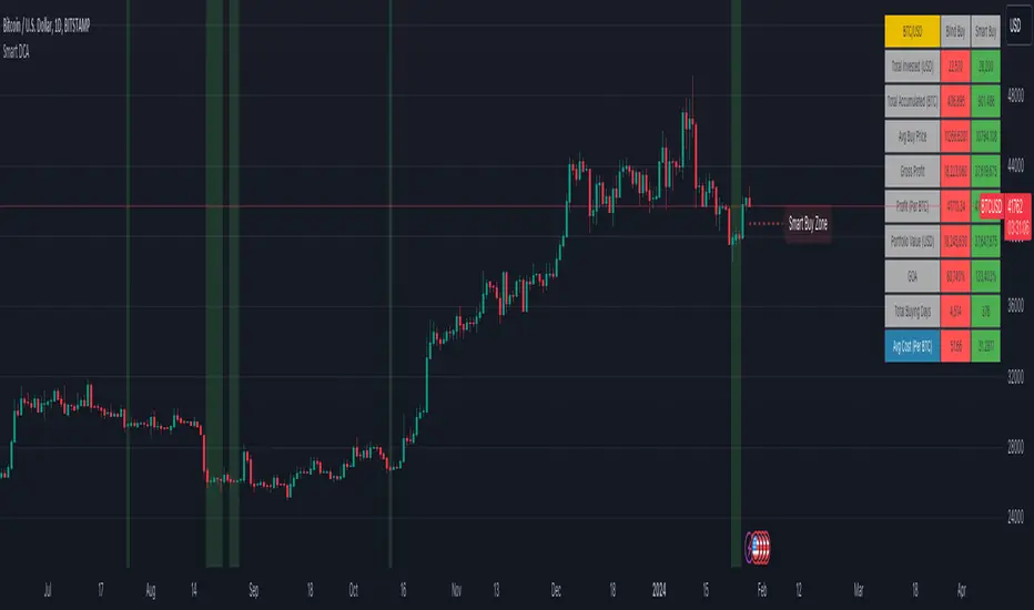
Autoback Grid Lab [trade_lexx]Autoback Grid Lab: Your personal laboratory for optimizing grid strategies.
Introduction
First of all, it is important to understand that Autoback Grid Lab is a powerful professional tool for backtesting and optimization, created specifically for traders using both grid strategies and regular take profit with stop loss.
The main purpose of this script is to save you weeks and months of manual testing and parameter selection. Instead of manually testing one combination of settings after another, Autoback Grid Lab automatically tests thousands of unique strategies on historical data, providing you with a comprehensive report on the most profitable and, more importantly, sustainable ones.
If you want to find mathematically sound, most effective settings for your grid strategy on a specific asset and timeframe, then this tool was created for you.
Key Features
My tool has functionality that transforms the process of finding the perfect strategy from a routine into an exciting exploration.
🧪 Mass testing of thousands of combinations
The script is able to systematically generate and run a huge number of unique combinations of parameters through the built-in simulator. You set the ranges, and the indicator does all the work, testing all possible options for the following grid settings:
* Number of safety orders (SO Count)
* Grid step (SO Step)
* Step Multiplier (SO Multiplier) for building nonlinear grids
* Martingale for controlling the volume of subsequent orders
* Take Profit (%)
* Stop Loss (%), with the possibility of calculating both from the entry point and from the dynamic breakeven line
* The volume of the base order (Volume BO) as a percentage of the deposit
🏆 Unique `FinalScore` rating system
Sorting strategies by net profit alone is a direct path to self—deception and choosing strategies that are "tailored" to history and will inevitably fail in real trading. To solve this problem, we have developed FinalScore, a comprehensive assessment of the sustainability and quality of the strategy.
How does it work?
FinalScore analyzes each combination not one by one, but by nine key performance metrics at once, including Net Profit, Drawdown, Profit Factor, WinRate, Sharpe coefficients, Sortino, Squid and Omega. Each of these indicators is normalized, that is, reduced to a single scale. Then, to test the strategy for strength, the system performs 30 iterations, each time assigning random weights to these 9 metrics. A strategy gets a high FinalScore only if it shows consistently high results under different evaluation criteria. This proves her reliability and reduces the likelihood that her success was an accident.
📈 Realistic backtesting engine
The test results are meaningless if they do not take into account the actual trading conditions. Our simulator simulates real trading as accurately as possible, taking into account:
* Leverage: Calculation of the required margin to open and hold positions.
* Commission: A percentage commission is charged each time an order is opened and closed.
* Slippage: The order execution price is adjusted by a set percentage to simulate real market conditions.
* Liquidation model: This is one of the most important functions. The script continuously monitors the equity of the account (capital + unrealized P&L). If equity falls below the level of the supporting margin (calculated from the current value of the position), the simulator forcibly closes the position, as it would happen on a real exchange. This eliminates unrealistic scenarios where the strategy survives after a huge drawdown.
🔌 Integration with external signals
The indicator operates in two modes:
1. `No Signal': Standard mode. The trading cycle starts immediately as soon as the previous one has been closed. Ideal for testing the "pure" mechanics of the grid.
2. `External Signal`: In this mode, a new trading cycle will start only when a signal is received from an external source. You can connect any other indicator (such as the RSI, MACD, or your own strategy) to the script and use it as a trigger to log in. This allows you to combine the power of a grid strategy with your own entry points.
📊 Interactive and informative results panel
Upon completion of the calculations, a detailed table with the TOP N best strategies appears on the screen, sorted according to your chosen criterion. For each strategy in the rating, you will see not only the key metrics (Profit, Drawdown, duration of transactions), but also all the parameters that led to this result. You can immediately take these settings and apply them in your trading.
Application Options: How To Solve Your Problems
Autoback Grid Lab is a flexible tool that can be adapted to solve various tasks, from complete grid optimization to fine—tuning existing strategies. Here are some key scenarios for its use:
1. Complete Optimization Of The Grid Strategy
This is the basic and most powerful mode of use. You can find the most efficient grid configuration for any asset from scratch.
* How to use: Set wide ranges for all key grid parameters ('SO Count`, SO Step, SO Multiplier, Martingale, TP, etc.).
* In the `No Signal` mode: You will find the most stable grid configuration that works as an independent, constantly active strategy, regardless of which-or entrance indicators.
* In the `External Signal` mode: You can connect your favorite indicator for input (for example, RSI, MACD or a complex author's script) and find the optimal grid parameters that best complement your input signals. This allows you to turn a simple signaling strategy into a full-fledged grid system.
2. Selecting the Optimal Take Profit and Stop Loss for Your Strategy
Do you already have an entry strategy, but you are not sure where it is best to put Take Profit and Stop Loss? Autoback Grid Lab can solve this problem as well.
* How to use:
1. Disable optimization of all grid parameters (uncheck SO Count, SO Step, Martingale, etc.). Set the Min value for SO Count to 0.
2. Set the ranges for iteration only for 'Take Profit` and `Stop Loss'.
3. Turn on the External Signal mode and connect your indicator with input signals.
* Result: The script will run your historical entry signals with hundreds of different TP and SL combinations and show you which stop order levels bring maximum profit with minimal risk specifically for your entry points.
3. Building a Secure Network with Risk Management
Many traders are afraid of grid strategies because of the risk of large drawdowns. With the help of the optimizer, you can purposefully find the parameters for such a grid, which includes mandatory risk management through Stop Loss.
* How to use: Enable and set the range for Stop Loss, along with other grid parameters. Don't forget to test both types of SL calculations (`From entry point` and `From breakeven line`) to determine which one works more efficiently.
* Result: You will find balanced strategies in which the grid parameters (number of orders, martingale) and the Stop Loss level are selected in such a way as to maximize profits without going beyond the acceptable risk level for you.
How To Use The Indicator (Step-By-Step Guide)
Working with the Autoback Grid Lab is a sequential process consisting of four main steps: from initial setup to analysis of the finished results. Follow this guide to get the most out of the tool.
Step 1: Initial Setup
1. Add the indicator to the chart of your chosen asset and timeframe.
2. Open the script settings. The first thing you should pay attention to is the ⚙️ Optimization Settings ⚙️ group.
3. Set the `Bars Count'. This parameter determines how much historical data will be used for testing.
* Important: The more bars you specify, the more statistically reliable the backtest results will be. We recommend using the maximum available value (25,000) to test strategies at different market phases.
* Consider: The indicator performs all calculations on the last historical bar. After applying the TradingView settings, it will take some time to load all the specified bars. The results table will appear only after the data is fully loaded. Don't worry if it doesn't appear instantly. And if an error occurs, simply switch the number of combinations to 990 and back to 1000 until the table appears.
Step 2: Optimization Configuration
At this stage, you define the "universe" of parameters that our algorithm will explore.
1. Set the search ranges (🛠 Optimization Parameters 🛠 group).
For each grid parameter that you want to optimize (for example, SO Count or `Take Profit'), you must specify three values:
* Min: The minimum value of the range.
* Max: The maximum value of the range.
* Step: The step with which the values from Min to Max will be traversed.
*Example:* If you set Min=5, Max=10, and Step=1 for SO Count, the script will test strategies with 5, 6, 7, 8, 9, and 10 safety orders.
* Tip for users: To get the first results quickly, start with a larger step (for example, TP from 0.5% to 2.5% in 0.5 increments instead of 0.1). After you identify the most promising areas, you can perform a deeper analysis by expanding the ranges around these values.
2. Set Up Money Management (Group `💰 Money Management Settings 💰`).
Fill in these fields with the values that best match your actual trading conditions. This is critically important for obtaining reliable results.
* Capital: Your initial deposit.
* Leverage: Leverage.
* Commission (%): Your trading commission as a percentage.
* Slippage (%): Expected slippage.
* Liquidation Level (%): The level of the supporting margin (MMR in %). For example, for Binance Futures, this value is usually between 0.4% and 2.5%, depending on the asset and position size. Specify this value for your exchange.
3. Select the Sorting Criterion and the Direction (Group `⚙️ Optimization Settings ⚙️').
* `Sort by': Specify the main criteria by which the best strategies will be selected and sorted. I strongly recommend using finalScore to find the most balanced and sustainable strategies.
* `Direction': Choose which trades to test: Long, Short or Both.
Step 3: Start Testing and Work with "Parts"
The total number of unique combinations generated based on your ranges can reach tens of millions. TradingView has technical limitations on the number of calculations that the script can perform at a time. To get around this, I implemented a "Parts" system.
1. What are `Part` and `Combinations in Part'?
* `Combinations in Part': This is the number of backtests that the script performs in one run (1000 by default).
* `Part`: This is the number of the "portion" of combinations that you want to test.
2. How does it work in practice?
* After you have everything set up, leave Part:1 and wait for the results table to appear. You will see the TOP N best strategies from the first thousand tested.
* Analyze them. Then, to check the next thousand combinations, just change the Part to 2 in the settings and click OK. The script will run a test for the next batch.
* Repeat this process by increasing the Part number (`3`, 4, 5...), until you reach the last available part.
* Where can I see the total number of parts? In the information row below the results table, you will find Total parts. This will help you figure out how many more tests are left to run.
Step 4: Analyze the Results in the Table
The results table is your main decision—making tool. It displays the best strategies found, sorted by the criteria you have chosen.
1. Study the performance metrics:
* Rating: Position in the rating.
* Profit %: Net profit as a percentage of the initial capital.
* Drawdown%: The maximum drawdown of the deposit for the entire test period.
* Max Length: The maximum duration of one transaction in days, hours and minutes.
* Trades: The total number of completed trades.
2. Examine the winning parameters:
* To the right of the performance metrics are columns showing the exact settings that led to this result ('SO Count`, SO Step, TP (%), etc.).
3. How to choose the best strategy?
* Don't chase after the maximum profit! The strategy with the highest profit often has the highest drawdown, which makes it extremely risky.
* Seek a balance. The ideal strategy is a compromise between high profitability, low drawdown (Drawdown) and the maximum length of trades acceptable to you (Max Length).
* finalScore was created to find this balance. Trust him — he often highlights not the most profitable, but the most stable and reliable options.
Detailed Description Of The Settings
This section serves as a complete reference for each parameter available in the script settings. The parameters are grouped in the same way as in the indicator interface for your convenience.
Group: ⚙️ Optimization Settings ⚙️
The main parameters governing the testing process are collected here.
* `Enable Optimizer': The main switch. Activates or deactivates all backtesting functionality.
* `Direction': Determines which way trades will be opened during the simulation.
* Long: Shopping only.
* Short: Sales only.
* Both: Testing in both directions. Important: This mode only works in conjunction with an External Signal, as the script needs an external signal to determine the direction for each specific transaction.
* `Signal Mode`: Controls the conditions for starting a new trading cycle (opening a base order).
* No Signal: A new cycle starts immediately after the previous one is completed. This mode is used to test "pure" grid mechanics without reference to market conditions.
* External Signal: A new cycle begins only when a signal is received from an external indicator connected via the Signal field.
* `Signal': A field for connecting an external signal source (works only in the `External Signal` mode). You can select any other indicator on the chart.
* For Long** trades, the signal is considered received if the value of the external indicator ** is greater than 0.
* For Short** trades, the signal is considered received if the value of the external indicator ** is less than 0.
* `Bars Count': Sets the depth of the history in the bars for the backtest. The maximum value (25000) provides the most reliable results.
* `Sort by`: A key criterion for selecting and ranking the best strategies in the final table.
* FinalScore: Recommended mode. A comprehensive assessment that takes into account 9 metrics to find the most balanced and sustainable strategies.
* Profit: Sort by net profit.
* Drawdown: Sort by minimum drawdown.
* Max Length: Sort by the minimum length of the longest transaction.
* `Combinations Count': Indicates how many of the best strategies (from 1 to 50) will be displayed in the results table.
* `Close last trade`: If this option is enabled, any active trade will be forcibly closed at the closing price of the last historical bar. For grid strategies, it is recommended to always enable this option in order to get the correct calculation of the final profit and eliminate grid strategies that have been stuck for a long time.
Group: 💰 Money Management Settings 💰
The parameters in this group determine the financial conditions of the simulation. Specify values that are as close as possible to your actual values in order to get reliable results.
* `Capital': The initial deposit amount for the simulation.
* `Leverage`: The leverage used to calculate the margin.
* `Slippage` (%): Simulates the difference between the expected and actual order execution price. The specified percentage will be applied to each transaction.
* `Commission` (%): The trading commission of your exchange as a percentage. It is charged at the execution of each order (both at opening and closing).
* `Liquidation Level' (%): Maintenance Margin Ratio. This is a critical parameter for a realistic test. Liquidation in the simulator occurs if the Equity of the account (Capital + Unrealized P&L) falls below the level of the supporting margin.
Group: 🛠 Optimization Parameters 🛠
This is the "heart" of the optimizer, where you set ranges for iterating through the grid parameters.
* `Part`: The portion number of the combinations to be tested. Start with 1, and then increment (`2`, 3, ...) sequentially to check all generated strategies.
* `Combinations in Part': The number of backtests performed at a time (in one "Part"). Increasing the value may speed up the process, but it may cause the script to error due to platform limitations. If an error occurs, it is recommended to switch to the step below and back.
Three fields are available for each of the following parameters (`SO Count`, SO Step, SO Multiplier, etc.):
* `Min`: Minimum value for testing.
* `Max': The maximum value for testing.
* `Step`: The step with which the values in the range from Min to Max will be iterated over.
There is also a checkbox for each parameter. If it is enabled, the parameter will be optimized in the specified range. If disabled, only one value specified in the Min field will be used for all tests.
* 'Stop Loss': In addition to the standard settings Min, Max, Step, it has an additional parameter:
* `Type`: Defines how the stop loss price is calculated.
* From entry point: The SL level is calculated once from the entry price (base order price).
* From breakeven line: The SL level is dynamically recalculated from the average position price after each new safety order is executed.
Group: ⚡️Filters⚡️
Filters allow you to filter out those results from the final table that do not meet your minimum requirements.
For each filter (`Max Profit`, Min Drawdown, `Min Trade Length`), you can:
1. Turn it on or off using the checkbox.
2. Select the comparison condition: Greater (More) or Less (Less).
3. Set a threshold value.
*Example:* If you set Less and 20 for the Min Drawdown filter, only those strategies with a maximum drawdown of less than 20% will be included in the final table.
Group: 🎨 Visual Settings 🎨
Here you can customize the appearance of the results table.
* `Position': Selects the position of the table on the screen (for example, Bottom Left — bottom left).
* `Font Size': The size of the text in the table.
* `Header Background / Data Background`: Background colors for the header and data cells.
* `Header Font Color / Data Font Color`: Text colors for the header and data cells.
Important Notes and Limitations
So that you can use the Autoback Grid Lab as efficiently and consciously as possible, please familiarize yourself with the following key features of its work.
1. It is a Tool for Analysis, not for Signals
It is extremely important to understand that this script does not generate trading signals in real time. Its sole purpose is to conduct in—depth research (**backtesting**) on historical data.
* The results you see in the table are a report on how a particular strategy would have worked in the past.
* The script does not provide alerts and does not draw entry/exit points on the chart for the current market situation.
* Your task is to take the best sets of parameters found during optimization and use them in your real trading, for example, when setting up a trading bot or in a manual trading system.
2. Features Of Calculations (This is not a "Repainting")
You will notice that the results table appears and is updated only once — when all historical bars on the chart are loaded. It does not change in real time with each tick of the price.
This is correct and intentional behavior.:
* To test thousands, and sometimes millions of combinations, the script needs to perform a huge amount of calculations. In the Pine Script™ environment, it is technically possible to do this only once, at the very last bar in history.
* The script does not show false historical signals, which then disappear or change. It provides a static report on the results of the simulation, which remains unchanged for a specific historical period.
3. Past Results do not Guarantee Future Results.
This is the golden rule of trading, and it fully applies to the results of backtesting. Successful strategy performance in the past is not a guarantee that it will be as profitable in the future. Market conditions, volatility and trends are constantly changing.
My tool, especially when sorting by finalScore, is aimed at finding statistically stable and reliable strategies to increase the likelihood of their success in the future. However, it is a tool for managing probabilities, not a crystal ball for predicting the future. Always use proper risk management.
4. Dependence on the Quality and Depth of the Story
The reliability of the results directly depends on the quantity and quality of the historical data on which the test was conducted.
* Always strive to use the maximum number of bars available (`Bars Count: 25,000`) so that your strategy is tested on different market cycles (rise, fall, flat).
* The results obtained on data for one month may differ dramatically from the results obtained on data for two years. The longer the testing period, the higher the confidence in the parameters found.
Conclusion
The Autoback Grid Lab is your personal research laboratory, designed to replace intuitive guesses and endless manual selection of settings with a systematic, data—driven approach. Experiment with different assets, timeframes, and settings ranges to find the unique combinations that best suit your trading style.

GKD-B Multi-Ticker Stepped Baseline [Loxx]Giga Kaleidoscope GKD-B Multi-Ticker Stepped Baseline is a Baseline module included in Loxx's "Giga Kaleidoscope Modularized Trading System".
This version of the GKD-B Baseline is designed specifically to support traders who wish to conduct GKD-BT Multi-Ticker Backtests with multiple tickers. This functionality is exclusive to the GKD-BT Multi-Ticker Backtests.
Traders have the capability to apply a filter to the selected moving average, leveraging various volatility metrics to enhance trend identification. This feature is tailored for traders favoring a gradual and consistent approach, enabling them to discern more sustainable trends. The system permits filtering for both the input data and the moving average results, requiring price movements to exceed a specific threshold—defined as multiples of the volatility—before acknowledging a trend change. This mechanism effectively reduces false signals caused by market noise and lateral movements. A distinctive aspect of this tool is its ability to adjust both price and moving average data based on volatility indicators like VIX, EUVIX, BVIV, and EVIV, among others. Understanding the time frame over which a volatility index is measured is crucial; for instance, VIX is measured on an annual basis, whereas BVIV and EVIV are based on a 30-day period. To accurately convert these measurements to a daily scale, users must input the correct "days per year" value: 252 for VIX and 30 for BVIV and EVIV. Future updates will introduce additional functionality to extend analysis across various time frames, but currently, this feature is solely available for daily time frame analysis.
█ GKD-B Multi-Ticker Stepped Baseline includes 65+ different moving averages:
Adaptive Moving Average - AMA
ADXvma - Average Directional Volatility Moving Average
Ahrens Moving Average
Alexander Moving Average - ALXMA
Deviation Scaled Moving Average - DSMA
Donchian
Double Exponential Moving Average - DEMA
Double Smoothed Exponential Moving Average - DSEMA
Double Smoothed FEMA - DSFEMA
Double Smoothed Range Weighted EMA - DSRWEMA
Double Smoothed Wilders EMA - DSWEMA
Double Weighted Moving Average - DWMA
Ehlers Optimal Tracking Filter - EOTF
Exponential Moving Average - EMA
Fast Exponential Moving Average - FEMA
Fractal Adaptive Moving Average - FRAMA
Generalized DEMA - GDEMA
Generalized Double DEMA - GDDEMA
Hull Moving Average (Type 1) - HMA1
Hull Moving Average (Type 2) - HMA2
Hull Moving Average (Type 3) - HMA3
Hull Moving Average (Type 4) - HMA4
IE /2 - Early T3 by Tim Tilson
Integral of Linear Regression Slope - ILRS
Kaufman Adaptive Moving Average - KAMA
Laguerre Filter
Leader Exponential Moving Average
Linear Regression Value - LSMA ( Least Squares Moving Average )
Linear Weighted Moving Average - LWMA
McGinley Dynamic
McNicholl EMA
Non-Lag Moving Average
Ocean NMA Moving Average - ONMAMA
One More Moving Average - OMA
Parabolic Weighted Moving Average
Probability Density Function Moving Average - PDFMA
Quadratic Regression Moving Average - QRMA
Regularized EMA - REMA
Range Weighted EMA - RWEMA
Recursive Moving Trendline
Simple Decycler - SDEC
Simple Jurik Moving Average - SJMA
Simple Moving Average - SMA
Sine Weighted Moving Average
Smoothed LWMA - SLWMA
Smoothed Moving Average - SMMA
Smoother
Super Smoother
T3
Three-pole Ehlers Butterworth
Three-pole Ehlers Smoother
Triangular Moving Average - TMA
Triple Exponential Moving Average - TEMA
Two-pole Ehlers Butterworth
Two-pole Ehlers smoother
Variable Index Dynamic Average - VIDYA
Variable Moving Average - VMA
Volume Weighted EMA - VEMA
Volume Weighted Moving Average - VWMA
Zero-Lag DEMA - Zero Lag Exponential Moving Average
Zero-Lag Moving Average
Zero Lag TEMA - Zero Lag Triple Exponential Moving Average
Geometric Mean Moving Average
Coral
Tether Lines
Range Filter
Triangle Moving Average Generalized
Ultinate Smoother
Adaptive Moving Average - AMA
The Adaptive Moving Average (AMA) is a moving average that changes its sensitivity to price moves depending on the calculated volatility. It becomes more sensitive during periods when the price is moving smoothly in a certain direction and becomes less sensitive when the price is volatile.
ADXvma - Average Directional Volatility Moving Average
Linnsoft's ADXvma formula is a volatility-based moving average, with the volatility being determined by the value of the ADX indicator.
The ADXvma has the SMA in Chande's CMO replaced with an EMA , it then uses a few more layers of EMA smoothing before the "Volatility Index" is calculated.
A side effect is, those additional layers slow down the ADXvma when you compare it to Chande's Variable Index Dynamic Average VIDYA .
The ADXVMA provides support during uptrends and resistance during downtrends and will stay flat for longer, but will create some of the most accurate market signals when it decides to move.
Ahrens Moving Average
Richard D. Ahrens's Moving Average promises "Smoother Data" that isn't influenced by the occasional price spike. It works by using the Open and the Close in his formula so that the only time the Ahrens Moving Average will change is when the candlestick is either making new highs or new lows.
Alexander Moving Average - ALXMA
This Moving Average uses an elaborate smoothing formula and utilizes a 7 period Moving Average. It corresponds to fitting a second-order polynomial to seven consecutive observations. This moving average is rarely used in trading but is interesting as this Moving Average has been applied to diffusion indexes that tend to be very volatile.
Deviation Scaled Moving Average - DSMA
The Deviation-Scaled Moving Average is a data smoothing technique that acts like an exponential moving average with a dynamic smoothing coefficient. The smoothing coefficient is automatically updated based on the magnitude of price changes. In the Deviation-Scaled Moving Average, the standard deviation from the mean is chosen to be the measure of this magnitude. The resulting indicator provides substantial smoothing of the data even when price changes are small while quickly adapting to these changes.
Donchian
Donchian Channels are three lines generated by moving average calculations that comprise an indicator formed by upper and lower bands around a midrange or median band. The upper band marks the highest price of a security over N periods while the lower band marks the lowest price of a security over N periods.
Double Exponential Moving Average - DEMA
The Double Exponential Moving Average ( DEMA ) combines a smoothed EMA and a single EMA to provide a low-lag indicator. It's primary purpose is to reduce the amount of "lagging entry" opportunities, and like all Moving Averages, the DEMA confirms uptrends whenever price crosses on top of it and closes above it, and confirms downtrends when the price crosses under it and closes below it - but with significantly less lag.
Double Smoothed Exponential Moving Average - DSEMA
The Double Smoothed Exponential Moving Average is a lot less laggy compared to a traditional EMA . It's also considered a leading indicator compared to the EMA , and is best utilized whenever smoothness and speed of reaction to market changes are required.
Double Smoothed FEMA - DSFEMA
Same as the Double Exponential Moving Average (DEMA), but uses a faster version of EMA for its calculation.
Double Smoothed Range Weighted EMA - DSRWEMA
Range weighted exponential moving average (EMA) is, unlike the "regular" range weighted average calculated in a different way. Even though the basis - the range weighting - is the same, the way how it is calculated is completely different. By definition this type of EMA is calculated as a ratio of EMA of price*weight / EMA of weight. And the results are very different and the two should be considered as completely different types of averages. The higher than EMA to price changes responsiveness when the ranges increase remains in this EMA too and in those cases this EMA is clearly leading the "regular" EMA. This version includes double smoothing.
Double Smoothed Wilders EMA - DSWEMA
Welles Wilder was frequently using one "special" case of EMA (Exponential Moving Average) that is due to that fact (that he used it) sometimes called Wilder's EMA. This version is adding double smoothing to Wilder's EMA in order to make it "faster" (it is more responsive to market prices than the original) and is still keeping very smooth values.
Double Weighted Moving Average - DWMA
Double weighted moving average is an LWMA (Linear Weighted Moving Average). Instead of doing one cycle for calculating the LWMA, the indicator is made to cycle the loop 2 times. That produces a smoother values than the original LWMA
Ehlers Optimal Tracking Filter - EOTF
The Elher's Optimum Tracking Filter quickly adjusts rapid shifts in the price and yet is relatively smooth when the price has a sideways action. The operation of this filter is similar to Kaufman’s Adaptive Moving
Average
Exponential Moving Average - EMA
The EMA places more significance on recent data points and moves closer to price than the SMA ( Simple Moving Average ). It reacts faster to volatility due to its emphasis on recent data and is known for its ability to give greater weight to recent and more relevant data. The EMA is therefore seen as an enhancement over the SMA .
Fast Exponential Moving Average - FEMA
An Exponential Moving Average with a short look-back period.
Fractal Adaptive Moving Average - FRAMA
The Fractal Adaptive Moving Average by John Ehlers is an intelligent adaptive Moving Average which takes the importance of price changes into account and follows price closely enough to display significant moves whilst remaining flat if price ranges. The FRAMA does this by dynamically adjusting the look-back period based on the market's fractal geometry.
Generalized DEMA - GDEMA
The double exponential moving average (DEMA), was developed by Patrick Mulloy in an attempt to reduce the amount of lag time found in traditional moving averages. It was first introduced in the February 1994 issue of the magazine Technical Analysis of Stocks & Commodities in Mulloy's article "Smoothing Data with Faster Moving Averages.". Instead of using fixed multiplication factor in the final DEMA formula, the generalized version allows you to change it. By varying the "volume factor" form 0 to 1 you apply different multiplications and thus producing DEMA with different "speed" - the higher the volume factor is the "faster" the DEMA will be (but also the slope of it will be less smooth). The volume factor is limited in the calculation to 1 since any volume factor that is larger than 1 is increasing the overshooting to the extent that some volume factors usage makes the indicator unusable.
Generalized Double DEMA - GDDEMA
The double exponential moving average (DEMA), was developed by Patrick Mulloy in an attempt to reduce the amount of lag time found in traditional moving averages. It was first introduced in the February 1994 issue of the magazine Technical Analysis of Stocks & Commodities in Mulloy's article "Smoothing Data with Faster Moving Averages''. This is an extension of the Generalized DEMA using Tim Tillsons (the inventor of T3) idea, and is using GDEMA of GDEMA for calculation (which is the "middle step" of T3 calculation). Since there are no versions showing that middle step, this version covers that too. The result is smoother than Generalized DEMA, but is less smooth than T3 - one has to do some experimenting in order to find the optimal way to use it, but in any case, since it is "faster" than the T3 (Tim Tillson T3) and still smooth, it looks like a good compromise between speed and smoothness.
Hull Moving Average (Type 1) - HMA1
Alan Hull's HMA makes use of weighted moving averages to prioritize recent values and greatly reduce lag whilst maintaining the smoothness of a traditional Moving Average. For this reason, it's seen as a well-suited Moving Average for identifying entry points. This version uses SMA for smoothing.
Hull Moving Average (Type 2) - HMA2
Alan Hull's HMA makes use of weighted moving averages to prioritize recent values and greatly reduce lag whilst maintaining the smoothness of a traditional Moving Average. For this reason, it's seen as a well-suited Moving Average for identifying entry points. This version uses EMA for smoothing.
Hull Moving Average (Type 3) - HMA3
Alan Hull's HMA makes use of weighted moving averages to prioritize recent values and greatly reduce lag whilst maintaining the smoothness of a traditional Moving Average. For this reason, it's seen as a well-suited Moving Average for identifying entry points. This version uses LWMA for smoothing.
Hull Moving Average (Type 4) - HMA4
Alan Hull's HMA makes use of weighted moving averages to prioritize recent values and greatly reduce lag whilst maintaining the smoothness of a traditional Moving Average. For this reason, it's seen as a well-suited Moving Average for identifying entry points. This version uses SMMA for smoothing.
IE /2 - Early T3 by Tim Tilson and T3 new
The T3 moving average is a type of technical indicator used in financial analysis to identify trends in price movements. It is similar to the Exponential Moving Average (EMA) and the Double Exponential Moving Average (DEMA), but uses a different smoothing algorithm.
The T3 moving average is calculated using a series of exponential moving averages that are designed to filter out noise and smooth the data. The resulting smoothed data is then weighted with a non-linear function to produce a final output that is more responsive to changes in trend direction.
The T3 moving average can be customized by adjusting the length of the moving average, as well as the weighting function used to smooth the data. It is commonly used in conjunction with other technical indicators as part of a larger trading strategy.
Integral of Linear Regression Slope - ILRS
A Moving Average where the slope of a linear regression line is simply integrated as it is fitted in a moving window of length N (natural numbers in maths) across the data. The derivative of ILRS is the linear regression slope. ILRS is not the same as a SMA ( Simple Moving Average ) of length N, which is actually the midpoint of the linear regression line as it moves across the data.
Kaufman Adaptive Moving Average - KAMA
Developed by Perry Kaufman, Kaufman's Adaptive Moving Average (KAMA) is a moving average designed to account for market noise or volatility. KAMA will closely follow prices when the price swings are relatively small and the noise is low.
Laguerre Filter
The Laguerre Filter is a smoothing filter which is based on Laguerre polynomials. The filter requires the current price, three prior prices, a user defined factor called Alpha to fill its calculation.
Adjusting the Alpha coefficient is used to increase or decrease its lag and its smoothness.
Leader Exponential Moving Average
The Leader EMA was created by Giorgos E. Siligardos who created a Moving Average which was able to eliminate lag altogether whilst maintaining some smoothness. It was first described during his research paper "MACD Leader" where he applied this to the MACD to improve its signals and remove its lagging issue. This filter uses his leading MACD's "modified EMA" and can be used as a zero lag filter.
Linear Regression Value - LSMA ( Least Squares Moving Average )
LSMA as a Moving Average is based on plotting the end point of the linear regression line. It compares the current value to the prior value and a determination is made of a possible trend, eg. the linear regression line is pointing up or down.
Linear Weighted Moving Average - LWMA
LWMA reacts to price quicker than the SMA and EMA . Although it's similar to the Simple Moving Average , the difference is that a weight coefficient is multiplied to the price which means the most recent price has the highest weighting, and each prior price has progressively less weight. The weights drop in a linear fashion.
McGinley Dynamic
John McGinley created this Moving Average to track prices better than traditional Moving Averages. It does this by incorporating an automatic adjustment factor into its formula, which speeds (or slows) the indicator in trending, or ranging, markets.
McNicholl EMA
Dennis McNicholl developed this Moving Average to use as his center line for his "Better Bollinger Bands" indicator and was successful because it responded better to volatility changes over the standard SMA and managed to avoid common whipsaws.
Non-lag moving average
The Non Lag Moving average follows price closely and gives very quick signals as well as early signals of price change. As a standalone Moving Average, it should not be used on its own, but as an additional confluence tool for early signals.
Ocean NMA Moving Average - ONMAMA
Created by Jim Sloman, the NMA is a moving average that automatically adjusts to volatility without being programmed to do so. For more info, read his guide "Ocean Theory, an Introduction"
One More Moving Average (OMA)
The One More Moving Average (OMA) is a technical indicator that calculates a series of Jurik-style moving averages in order to reduce noise and provide smoother price data. It uses six exponential moving averages to generate the final value, with the length of the moving averages determined by an adaptive algorithm that adjusts to the current market conditions. The algorithm calculates the average period by comparing the signal to noise ratio and using this value to determine the length of the moving averages. The resulting values are used to generate the final value of the OMA, which can be used to identify trends and potential changes in trend direction.
Parabolic Weighted Moving Average
The Parabolic Weighted Moving Average is a variation of the Linear Weighted Moving Average . The Linear Weighted Moving Average calculates the average by assigning different weights to each element in its calculation. The Parabolic Weighted Moving Average is a variation that allows weights to be changed to form a parabolic curve. It is done simply by using the Power parameter of this indicator.
Probability Density Function Moving Average - PDFMA
Probability density function based MA is a sort of weighted moving average that uses probability density function to calculate the weights. By its nature it is similar to a lot of digital filters.
Quadratic Regression Moving Average - QRMA
A quadratic regression is the process of finding the equation of the parabola that best fits a set of data. This moving average is an obscure concept that was posted to Forex forums in around 2008.
Regularized EMA - REMA
The regularized exponential moving average (REMA) by Chris Satchwell is a variation on the EMA (see Exponential Moving Average) designed to be smoother but not introduce too much extra lag.
Range Weighted EMA - RWEMA
This indicator is a variation of the range weighted EMA. The variation comes from a possible need to make that indicator a bit less "noisy" when it comes to slope changes. The method used for calculating this variation is the method described by Lee Leibfarth in his article "Trading With An Adaptive Price Zone".
Recursive Moving Trendline
Dennis Meyers's Recursive Moving Trendline uses a recursive (repeated application of a rule) polynomial fit, a technique that uses a small number of past values estimations of price and today's price to predict tomorrow's price.
Simple Decycler - SDEC
The Ehlers Simple Decycler study is a virtually zero-lag technical indicator proposed by John F. Ehlers. The original idea behind this study (and several others created by John F. Ehlers) is that market data can be considered a continuum of cycle periods with different cycle amplitudes. Thus, trending periods can be considered segments of longer cycles, or, in other words, low-frequency segments. Applying the right filter might help identify these segments.
Simple Loxx Moving Average - SLMA
A three stage moving average combining an adaptive EMA, a Kalman Filter, and a Kauffman adaptive filter.
Simple Moving Average - SMA
The SMA calculates the average of a range of prices by adding recent prices and then dividing that figure by the number of time periods in the calculation average. It is the most basic Moving Average which is seen as a reliable tool for starting off with Moving Average studies. As reliable as it may be, the basic moving average will work better when it's enhanced into an EMA .
Sine Weighted Moving Average
The Sine Weighted Moving Average assigns the most weight at the middle of the data set. It does this by weighting from the first half of a Sine Wave Cycle and the most weighting is given to the data in the middle of that data set. The Sine WMA closely resembles the TMA (Triangular Moving Average).
Smoothed LWMA - SLWMA
A smoothed version of the LWMA
Smoothed Moving Average - SMMA
The Smoothed Moving Average is similar to the Simple Moving Average ( SMA ), but aims to reduce noise rather than reduce lag. SMMA takes all prices into account and uses a long lookback period. Due to this, it's seen as an accurate yet laggy Moving Average.
Smoother
The Smoother filter is a faster-reacting smoothing technique which generates considerably less lag than the SMMA ( Smoothed Moving Average ). It gives earlier signals but can also create false signals due to its earlier reactions. This filter is sometimes wrongly mistaken for the superior Jurik Smoothing algorithm.
Super Smoother
The Super Smoother filter uses John Ehlers’s “Super Smoother” which consists of a Two pole Butterworth filter combined with a 2-bar SMA ( Simple Moving Average ) that suppresses the 22050 Hz Nyquist frequency: A characteristic of a sampler, which converts a continuous function or signal into a discrete sequence.
Three-pole Ehlers Butterworth
The 3 pole Ehlers Butterworth (as well as the Two pole Butterworth) are both superior alternatives to the EMA and SMA . They aim at producing less lag whilst maintaining accuracy. The 2 pole filter will give you a better approximation for price, whereas the 3 pole filter has superior smoothing.
Three-pole Ehlers smoother
The 3 pole Ehlers smoother works almost as close to price as the above mentioned 3 Pole Ehlers Butterworth. It acts as a strong baseline for signals but removes some noise. Side by side, it hardly differs from the Three Pole Ehlers Butterworth but when examined closely, it has better overshoot reduction compared to the 3 pole Ehlers Butterworth.
Triangular Moving Average - TMA
The TMA is similar to the EMA but uses a different weighting scheme. Exponential and weighted Moving Averages will assign weight to the most recent price data. Simple moving averages will assign the weight equally across all the price data. With a TMA (Triangular Moving Average), it is double smoother (averaged twice) so the majority of the weight is assigned to the middle portion of the data.
Triple Exponential Moving Average - TEMA
The TEMA uses multiple EMA calculations as well as subtracting lag to create a tool which can be used for scalping pullbacks. As it follows price closely, its signals are considered very noisy and should only be used in extremely fast-paced trading conditions.
Two-pole Ehlers Butterworth
The 2 pole Ehlers Butterworth (as well as the three pole Butterworth mentioned above) is another filter that cuts out the noise and follows the price closely. The 2 pole is seen as a faster, leading filter over the 3 pole and follows price a bit more closely. Analysts will utilize both a 2 pole and a 3 pole Butterworth on the same chart using the same period, but having both on chart allows its crosses to be traded.
Two-pole Ehlers smoother
A smoother version of the Two pole Ehlers Butterworth. This filter is the faster version out of the 3 pole Ehlers Butterworth. It does a decent job at cutting out market noise whilst emphasizing a closer following to price over the 3 pole Ehlers .
Variable Index Dynamic Average - VIDYA
Variable Index Dynamic Average Technical Indicator ( VIDYA ) was developed by Tushar Chande. It is an original method of calculating the Exponential Moving Average ( EMA ) with the dynamically changing period of averaging.
Variable Moving Average - VMA
The Variable Moving Average (VMA) is a study that uses an Exponential Moving Average being able to automatically adjust its smoothing factor according to the market volatility.
Volume Weighted EMA - VEMA
An EMA that uses a volume and price weighted calculation instead of the standard price input.
Volume Weighted Moving Average - VWMA
A Volume Weighted Moving Average is a moving average where more weight is given to bars with heavy volume than with light volume. Thus the value of the moving average will be closer to where most trading actually happened than it otherwise would be without being volume weighted.
Zero-Lag DEMA - Zero Lag Double Exponential Moving Average
John Ehlers's Zero Lag DEMA's aim is to eliminate the inherent lag associated with all trend following indicators which average a price over time. Because this is a Double Exponential Moving Average with Zero Lag, it has a tendency to overshoot and create a lot of false signals for swing trading. It can however be used for quick scalping or as a secondary indicator for confluence.
Zero-Lag Moving Average
The Zero Lag Moving Average is described by its creator, John Ehlers , as a Moving Average with absolutely no delay. And it's for this reason that this filter will cause a lot of abrupt signals which will not be ideal for medium to long-term traders. This filter is designed to follow price as close as possible whilst de-lagging data instead of basing it on regular data. The way this is done is by attempting to remove the cumulative effect of the Moving Average.
Zero-Lag TEMA - Zero Lag Triple Exponential Moving Average
Just like the Zero Lag DEMA , this filter will give you the fastest signals out of all the Zero Lag Moving Averages. This is useful for scalping but dangerous for medium to long-term traders, especially during market Volatility and news events. Having no lag, this filter also has no smoothing in its signals and can cause some very bizarre behavior when applied to certain indicators.
█ Volatility Goldie Locks Zone
This volatility filter is the standard first pass filter that is used for all NNFX systems despite the additional volatility/volume filter used in step 5. For this filter, price must fall into a range of maximum and minimum values calculated using multiples of volatility. Unlike the standard NNFX systems, this version of volatility filtering is separated from the core Baseline and uses it's own moving average with Loxx's Exotic Source Types.
█ Volatility Types included
The GKD system utilizes volatility-based take profits and stop losses. Each take profit and stop loss is calculated as a multiple of volatility. You can change the values of the multipliers in the settings as well.
This module includes 17 types of volatility:
Close-to-Close
Parkinson
Garman-Klass
Rogers-Satchell
Yang-Zhang
Garman-Klass-Yang-Zhang
Exponential Weighted Moving Average
Standard Deviation of Log Returns
Pseudo GARCH(2,2)
Average True Range
True Range Double
Standard Deviation
Adaptive Deviation
Median Absolute Deviation
Efficiency-Ratio Adaptive ATR
Mean Absolute Deviation
Static Percent
Various volatility estimators and indicators that investors and traders can use to measure the dispersion or volatility of a financial instrument's price. Each estimator has its strengths and weaknesses, and the choice of estimator should depend on the specific needs and circumstances of the user.
Volatility Ticker Selection
Import volatility tickers like VIX, EUVIX, BVIV, and EVIV.
Close-to-Close
Close-to-Close volatility is a classic and widely used volatility measure, sometimes referred to as historical volatility.
Volatility is an indicator of the speed of a stock price change. A stock with high volatility is one where the price changes rapidly and with a larger amplitude. The more volatile a stock is, the riskier it is.
Close-to-close historical volatility is calculated using only a stock's closing prices. It is the simplest volatility estimator. However, in many cases, it is not precise enough. Stock prices could jump significantly during a trading session and return to the opening value at the end. That means that a considerable amount of price information is not taken into account by close-to-close volatility.
Despite its drawbacks, Close-to-Close volatility is still useful in cases where the instrument doesn't have intraday prices. For example, mutual funds calculate their net asset values daily or weekly, and thus their prices are not suitable for more sophisticated volatility estimators.
Parkinson
Parkinson volatility is a volatility measure that uses the stock’s high and low price of the day.
The main difference between regular volatility and Parkinson volatility is that the latter uses high and low prices for a day, rather than only the closing price. This is useful as close-to-close prices could show little difference while large price movements could have occurred during the day. Thus, Parkinson's volatility is considered more precise and requires less data for calculation than close-to-close volatility.
One drawback of this estimator is that it doesn't take into account price movements after the market closes. Hence, it systematically undervalues volatility. This drawback is addressed in the Garman-Klass volatility estimator.
Garman-Klass
Garman-Klass is a volatility estimator that incorporates open, low, high, and close prices of a security.
Garman-Klass volatility extends Parkinson's volatility by taking into account the opening and closing prices. As markets are most active during the opening and closing of a trading session, it makes volatility estimation more accurate.
Garman and Klass also assumed that the process of price change follows a continuous diffusion process (Geometric Brownian motion). However, this assumption has several drawbacks. The method is not robust for opening jumps in price and trend movements.
Despite its drawbacks, the Garman-Klass estimator is still more effective than the basic formula since it takes into account not only the price at the beginning and end of the time interval but also intraday price extremes.
Researchers Rogers and Satchell have proposed a more efficient method for assessing historical volatility that takes into account price trends. See Rogers-Satchell Volatility for more detail.
Rogers-Satchell
Rogers-Satchell is an estimator for measuring the volatility of securities with an average return not equal to zero.
Unlike Parkinson and Garman-Klass estimators, Rogers-Satchell incorporates a drift term (mean return not equal to zero). As a result, it provides better volatility estimation when the underlying is trending.
The main disadvantage of this method is that it does not take into account price movements between trading sessions. This leads to an underestimation of volatility since price jumps periodically occur in the market precisely at the moments between sessions.
A more comprehensive estimator that also considers the gaps between sessions was developed based on the Rogers-Satchel formula in the 2000s by Yang-Zhang. See Yang Zhang Volatility for more detail.
Yang-Zhang
Yang Zhang is a historical volatility estimator that handles both opening jumps and the drift and has a minimum estimation error.
Yang-Zhang volatility can be thought of as a combination of the overnight (close-to-open volatility) and a weighted average of the Rogers-Satchell volatility and the day’s open-to-close volatility. It is considered to be 14 times more efficient than the close-to-close estimator.
Garman-Klass-Yang-Zhang
Garman-Klass-Yang-Zhang (GKYZ) volatility estimator incorporates the returns of open, high, low, and closing prices in its calculation.
GKYZ volatility estimator takes into account overnight jumps but not the trend, i.e., it assumes that the underlying asset follows a Geometric Brownian Motion (GBM) process with zero drift. Therefore, the GKYZ volatility estimator tends to overestimate the volatility when the drift is different from zero. However, for a GBM process, this estimator is eight times more efficient than the close-to-close volatility estimator.
Exponential Weighted Moving Average
The Exponentially Weighted Moving Average (EWMA) is a quantitative or statistical measure used to model or describe a time series. The EWMA is widely used in finance, with the main applications being technical analysis and volatility modeling.
The moving average is designed such that older observations are given lower weights. The weights decrease exponentially as the data point gets older – hence the name exponentially weighted.
The only decision a user of the EWMA must make is the parameter lambda. The parameter decides how important the current observation is in the calculation of the EWMA. The higher the value of lambda, the more closely the EWMA tracks the original time series.
Standard Deviation of Log Returns
This is the simplest calculation of volatility. It's the standard deviation of ln(close/close(1)).
Pseudo GARCH(2,2)
This is calculated using a short- and long-run mean of variance multiplied by ?.
avg(var;M) + (1 ? ?) avg(var;N) = 2?var/(M+1-(M-1)L) + 2(1-?)var/(M+1-(M-1)L)
Solving for ? can be done by minimizing the mean squared error of estimation; that is, regressing L^-1var - avg(var; N) against avg(var; M) - avg(var; N) and using the resulting beta estimate as ?.
Average True Range
The average true range (ATR) is a technical analysis indicator, introduced by market technician J. Welles Wilder Jr. in his book New Concepts in Technical Trading Systems, that measures market volatility by decomposing the entire range of an asset price for that period.
The true range indicator is taken as the greatest of the following: current high less the current low; the absolute value of the current high less the previous close; and the absolute value of the current low less the previous close. The ATR is then a moving average, generally using 14 days, of the true ranges.
True Range Double
A special case of ATR that attempts to correct for volatility skew.
Standard Deviation
Standard deviation is a statistic that measures the dispersion of a dataset relative to its mean and is calculated as the square root of the variance. The standard deviation is calculated as the square root of variance by determining each data point's deviation relative to the mean. If the data points are further from the mean, there is a higher deviation within the data set; thus, the more spread out the data, the higher the standard deviation.
Adaptive Deviation
By definition, the Standard Deviation (STD, also represented by the Greek letter sigma ? or the Latin letter s) is a measure that is used to quantify the amount of variation or dispersion of a set of data values. In technical analysis, we usually use it to measure the level of current volatility.
Standard Deviation is based on Simple Moving Average calculation for mean value. This version of standard deviation uses the properties of EMA to calculate what can be called a new type of deviation, and since it is based on EMA, we can call it EMA deviation. Additionally, Perry Kaufman's efficiency ratio is used to make it adaptive (since all EMA type calculations are nearly perfect for adapting).
The difference when compared to the standard is significant--not just because of EMA usage, but the efficiency ratio makes it a "bit more logical" in very volatile market conditions.
Median Absolute Deviation
The median absolute deviation is a measure of statistical dispersion. Moreover, the MAD is a robust statistic, being more resilient to outliers in a data set than the standard deviation. In the standard deviation, the distances from the mean are squared, so large deviations are weighted more heavily, and thus outliers can heavily influence it. In the MAD, the deviations of a small number of outliers are irrelevant.
Because the MAD is a more robust estimator of scale than the sample variance or standard deviation, it works better with distributions without a mean or variance, such as the Cauchy distribution.
For this indicator, a manual recreation of the quantile function in Pine Script is used. This is so users have a full inside view into how this is calculated.
Efficiency-Ratio Adaptive ATR
Average True Range (ATR) is a widely used indicator for many occasions in technical analysis. It is calculated as the RMA of the true range. This version adds a "twist": it uses Perry Kaufman's Efficiency Ratio to calculate adaptive true range.
Mean Absolute Deviation
The mean absolute deviation (MAD) is a measure of variability that indicates the average distance between observations and their mean. MAD uses the original units of the data, which simplifies interpretation. Larger values signify that the data points spread out further from the average. Conversely, lower values correspond to data points bunching closer to it. The mean absolute deviation is also known as the mean deviation and average absolute deviation.
This definition of the mean absolute deviation sounds similar to the standard deviation (SD). While both measure variability, they have different calculations. In recent years, some proponents of MAD have suggested that it replace the SD as the primary measure because it is a simpler concept that better fits real life.
█ Giga Kaleidoscope Modularized Trading System
Core components of an NNFX algorithmic trading strategy
The NNFX algorithm is built on the principles of trend, momentum, and volatility. There are six core components in the NNFX trading algorithm:
1. Volatility - price volatility; e.g., Average True Range, True Range Double, Close-to-Close, etc.
2. Baseline - a moving average to identify price trend
3. Confirmation 1 - a technical indicator used to identify trends
4. Confirmation 2 - a technical indicator used to identify trends
5. Continuation - a technical indicator used to identify trends
6. Volatility/Volume - a technical indicator used to identify volatility/volume breakouts/breakdown
7. Exit - a technical indicator used to determine when a trend is exhausted
8. Metamorphosis - a technical indicator that produces a compound signal from the combination of other GKD indicators*
*(not part of the NNFX algorithm)
What is Volatility in the NNFX trading system?
In the NNFX (No Nonsense Forex) trading system, ATR (Average True Range) is typically used to measure the volatility of an asset. It is used as a part of the system to help determine the appropriate stop loss and take profit levels for a trade. ATR is calculated by taking the average of the true range values over a specified period.
True range is calculated as the maximum of the following values:
-Current high minus the current low
-Absolute value of the current high minus the previous close
-Absolute value of the current low minus the previous close
ATR is a dynamic indicator that changes with changes in volatility. As volatility increases, the value of ATR increases, and as volatility decreases, the value of ATR decreases. By using ATR in NNFX system, traders can adjust their stop loss and take profit levels according to the volatility of the asset being traded. This helps to ensure that the trade is given enough room to move, while also minimizing potential losses.
Other types of volatility include True Range Double (TRD), Close-to-Close, and Garman-Klass
What is a Baseline indicator?
The baseline is essentially a moving average, and is used to determine the overall direction of the market.
The baseline in the NNFX system is used to filter out trades that are not in line with the long-term trend of the market. The baseline is plotted on the chart along with other indicators, such as the Moving Average (MA), the Relative Strength Index (RSI), and the Average True Range (ATR).
Trades are only taken when the price is in the same direction as the baseline. For example, if the baseline is sloping upwards, only long trades are taken, and if the baseline is sloping downwards, only short trades are taken. This approach helps to ensure that trades are in line with the overall trend of the market, and reduces the risk of entering trades that are likely to fail.
By using a baseline in the NNFX system, traders can have a clear reference point for determining the overall trend of the market, and can make more informed trading decisions. The baseline helps to filter out noise and false signals, and ensures that trades are taken in the direction of the long-term trend.
What is a Confirmation indicator?
Confirmation indicators are technical indicators that are used to confirm the signals generated by primary indicators. Primary indicators are the core indicators used in the NNFX system, such as the Average True Range (ATR), the Moving Average (MA), and the Relative Strength Index (RSI).
The purpose of the confirmation indicators is to reduce false signals and improve the accuracy of the trading system. They are designed to confirm the signals generated by the primary indicators by providing additional information about the strength and direction of the trend.
Some examples of confirmation indicators that may be used in the NNFX system include the Bollinger Bands, the MACD (Moving Average Convergence Divergence), and the MACD Oscillator. These indicators can provide information about the volatility, momentum, and trend strength of the market, and can be used to confirm the signals generated by the primary indicators.
In the NNFX system, confirmation indicators are used in combination with primary indicators and other filters to create a trading system that is robust and reliable. By using multiple indicators to confirm trading signals, the system aims to reduce the risk of false signals and improve the overall profitability of the trades.
What is a Continuation indicator?
In the NNFX (No Nonsense Forex) trading system, a continuation indicator is a technical indicator that is used to confirm a current trend and predict that the trend is likely to continue in the same direction. A continuation indicator is typically used in conjunction with other indicators in the system, such as a baseline indicator, to provide a comprehensive trading strategy.
What is a Volatility/Volume indicator?
Volume indicators, such as the On Balance Volume (OBV), the Chaikin Money Flow (CMF), or the Volume Price Trend (VPT), are used to measure the amount of buying and selling activity in a market. They are based on the trading volume of the market, and can provide information about the strength of the trend. In the NNFX system, volume indicators are used to confirm trading signals generated by the Moving Average and the Relative Strength Index. Volatility indicators include Average Direction Index, Waddah Attar, and Volatility Ratio. In the NNFX trading system, volatility is a proxy for volume and vice versa.
By using volume indicators as confirmation tools, the NNFX trading system aims to reduce the risk of false signals and improve the overall profitability of trades. These indicators can provide additional information about the market that is not captured by the primary indicators, and can help traders to make more informed trading decisions. In addition, volume indicators can be used to identify potential changes in market trends and to confirm the strength of price movements.
What is an Exit indicator?
The exit indicator is used in conjunction with other indicators in the system, such as the Moving Average (MA), the Relative Strength Index (RSI), and the Average True Range (ATR), to provide a comprehensive trading strategy.
The exit indicator in the NNFX system can be any technical indicator that is deemed effective at identifying optimal exit points. Examples of exit indicators that are commonly used include the Parabolic SAR, and the Average Directional Index (ADX).
The purpose of the exit indicator is to identify when a trend is likely to reverse or when the market conditions have changed, signaling the need to exit a trade. By using an exit indicator, traders can manage their risk and prevent significant losses.
In the NNFX system, the exit indicator is used in conjunction with a stop loss and a take profit order to maximize profits and minimize losses. The stop loss order is used to limit the amount of loss that can be incurred if the trade goes against the trader, while the take profit order is used to lock in profits when the trade is moving in the trader's favor.
Overall, the use of an exit indicator in the NNFX trading system is an important component of a comprehensive trading strategy. It allows traders to manage their risk effectively and improve the profitability of their trades by exiting at the right time.
What is an Metamorphosis indicator?
The concept of a metamorphosis indicator involves the integration of two or more GKD indicators to generate a compound signal. This is achieved by evaluating the accuracy of each indicator and selecting the signal from the indicator with the highest accuracy. As an illustration, let's consider a scenario where we calculate the accuracy of 10 indicators and choose the signal from the indicator that demonstrates the highest accuracy.
The resulting output from the metamorphosis indicator can then be utilized in a GKD-BT backtest by occupying a slot that aligns with the purpose of the metamorphosis indicator. The slot can be a GKD-B, GKD-C, or GKD-E slot, depending on the specific requirements and objectives of the indicator. This allows for seamless integration and utilization of the compound signal within the GKD-BT framework.
How does Loxx's GKD (Giga Kaleidoscope Modularized Trading System) implement the NNFX algorithm outlined above?
Loxx's GKD v2.0 system has five types of modules (indicators/strategies). These modules are:
1. GKD-BT - Backtesting module (Volatility, Number 1 in the NNFX algorithm)
2. GKD-B - Baseline module (Baseline and Volatility/Volume, Numbers 1 and 2 in the NNFX algorithm)
3. GKD-C - Confirmation 1/2 and Continuation module (Confirmation 1/2 and Continuation, Numbers 3, 4, and 5 in the NNFX algorithm)
4. GKD-V - Volatility/Volume module (Confirmation 1/2, Number 6 in the NNFX algorithm)
5. GKD-E - Exit module (Exit, Number 7 in the NNFX algorithm)
6. GKD-M - Metamorphosis module (Metamorphosis, Number 8 in the NNFX algorithm, but not part of the NNFX algorithm)
(additional module types will added in future releases)
Each module interacts with every module by passing data to A backtest module wherein the various components of the GKD system are combined to create a trading signal.
That is, the Baseline indicator passes its data to Volatility/Volume. The Volatility/Volume indicator passes its values to the Confirmation 1 indicator. The Confirmation 1 indicator passes its values to the Confirmation 2 indicator. The Confirmation 2 indicator passes its values to the Continuation indicator. The Continuation indicator passes its values to the Exit indicator, and finally, the Exit indicator passes its values to the Backtest strategy.
This chaining of indicators requires that each module conform to Loxx's GKD protocol, therefore allowing for the testing of every possible combination of technical indicators that make up the six components of the NNFX algorithm.
What does the application of the GKD trading system look like?
Example trading system:
Backtest: Multi-Ticker CC Backtest
Baseline: Hull Moving Average
Volatility/Volume: Hurst Exponent
Confirmation 1: Advance Trend Pressure as shown on the chart above
Confirmation 2: uf2018
Continuation: Coppock Curve
Exit: Rex Oscillator
Metamorphosis: Baseline Optimizer
Each GKD indicator is denoted with a module identifier of either: GKD-BT, GKD-B, GKD-C, GKD-V, GKD-M, or GKD-E. This allows traders to understand to which module each indicator belongs and where each indicator fits into the GKD system.
█ Giga Kaleidoscope Modularized Trading System Signals
Standard Entry
1. GKD-C Confirmation gives signal
2. Baseline agrees
3. Price inside Goldie Locks Zone Minimum
4. Price inside Goldie Locks Zone Maximum
5. Confirmation 2 agrees
6. Volatility/Volume agrees
1-Candle Standard Entry
1a. GKD-C Confirmation gives signal
2a. Baseline agrees
3a. Price inside Goldie Locks Zone Minimum
4a. Price inside Goldie Locks Zone Maximum
Next Candle
1b. Price retraced
2b. Baseline agrees
3b. Confirmation 1 agrees
4b. Confirmation 2 agrees
5b. Volatility/Volume agrees
Baseline Entry
1. GKD-B Baseline gives signal
2. Confirmation 1 agrees
3. Price inside Goldie Locks Zone Minimum
4. Price inside Goldie Locks Zone Maximum
5. Confirmation 2 agrees
6. Volatility/Volume agrees
7. Confirmation 1 signal was less than 'Maximum Allowable PSBC Bars Back' prior
1-Candle Baseline Entry
1a. GKD-B Baseline gives signal
2a. Confirmation 1 agrees
3a. Price inside Goldie Locks Zone Minimum
4a. Price inside Goldie Locks Zone Maximum
5a. Confirmation 1 signal was less than 'Maximum Allowable PSBC Bars Back' prior
Next Candle
1b. Price retraced
2b. Baseline agrees
3b. Confirmation 1 agrees
4b. Confirmation 2 agrees
5b. Volatility/Volume agrees
Volatility/Volume Entry
1. GKD-V Volatility/Volume gives signal
2. Confirmation 1 agrees
3. Price inside Goldie Locks Zone Minimum
4. Price inside Goldie Locks Zone Maximum
5. Confirmation 2 agrees
6. Baseline agrees
7. Confirmation 1 signal was less than 7 candles prior
1-Candle Volatility/Volume Entry
1a. GKD-V Volatility/Volume gives signal
2a. Confirmation 1 agrees
3a. Price inside Goldie Locks Zone Minimum
4a. Price inside Goldie Locks Zone Maximum
5a. Confirmation 1 signal was less than 'Maximum Allowable PSVVC Bars Back' prior
Next Candle
1b. Price retraced
2b. Volatility/Volume agrees
3b. Confirmation 1 agrees
4b. Confirmation 2 agrees
5b. Baseline agrees
Confirmation 2 Entry
1. GKD-C Confirmation 2 gives signal
2. Confirmation 1 agrees
3. Price inside Goldie Locks Zone Minimum
4. Price inside Goldie Locks Zone Maximum
5. Volatility/Volume agrees
6. Baseline agrees
7. Confirmation 1 signal was less than 7 candles prior
1-Candle Confirmation 2 Entry
1a. GKD-C Confirmation 2 gives signal
2a. Confirmation 1 agrees
3a. Price inside Goldie Locks Zone Minimum
4a. Price inside Goldie Locks Zone Maximum
5a. Confirmation 1 signal was less than 'Maximum Allowable PSC2C Bars Back' prior
Next Candle
1b. Price retraced
2b. Confirmation 2 agrees
3b. Confirmation 1 agrees
4b. Volatility/Volume agrees
5b. Baseline agrees
PullBack Entry
1a. GKD-B Baseline gives signal
2a. Confirmation 1 agrees
3a. Price is beyond 1.0x Volatility of Baseline
Next Candle
1b. Price inside Goldie Locks Zone Minimum
2b. Price inside Goldie Locks Zone Maximum
3b. Confirmation 1 agrees
4b. Confirmation 2 agrees
5b. Volatility/Volume agrees
Continuation Entry
1. Standard Entry, 1-Candle Standard Entry, Baseline Entry, 1-Candle Baseline Entry, Volatility/Volume Entry, 1-Candle Volatility/Volume Entry, Confirmation 2 Entry, 1-Candle Confirmation 2 Entry, or Pullback entry triggered previously
2. Baseline hasn't crossed since entry signal trigger
4. Confirmation 1 agrees
5. Baseline agrees
6. Confirmation 2 agrees

Strategy Development Environment [BerlinCode42]Happy Trade,
Intro
What is New
Algebraic/Boolean Equation
Instruction Set for The Algebraic/Boolean Equation
Example
Usage
Settings Menu
Declaration for Tradingview House Rules on Script Publishing
Disclaimer
Conclusion
1. Intro
This is a rich equipped fork of my previous "Backtest any Indicator v5". And serves as the fitting backtester and trade strategy creation tool for my upcoming ANN Indicators (artificial neural network).
As the previous version this script has no trade signal generating code. The trade signals comes in by the five user settable input slots where the user plug-in external indicators. The final trade siganls go long etc are defined by a algebraic/boolean equation typed in as text in 4 terminals as shown in Image 0 . With this algebraic/boolean equations input the user can setup any trade logic as complex and fast and easy as never seen before here on TradingView.
Image 0
2. What is new
Input algebraic/boolean equations in text-form for go long, go short, exit long & exit short
Five input slots for external indicator signals
Equation tester
User settable signal delay for enter and exit trades
User selectable alternating trades filter
User settable exit long = enter short
Intrabar or trade only on bar closing
Time filter with duration input
User settable UTC Adjustment
Long and short trades possible
Two Take Profits with quantity setting
Trailing Stop
Webhook connection
3. Algebraic/Boolean Equation
This is where the magic happens. Unlike other backtesters that rely on drop-down menus to define trade signal equations—thus limiting the number of input signals and the complexity of logic—this script uses a string interpreter to solve equations. With this, you can develop your trade logic equations and add signals or conditions simply by writing them down in algebraic/boolean form.
The instruction set for this interpreter includes not only external input signals but also several internal values. These include BarTime, BarIndex, Open, High, Low, Close, True Range, Minimal Tick, Volume, and a signal that indicates whether there is an open trade (long, short, or none). You can also reference the values of past bars for all these inputs and, of course, use constant values in your equations. There is a sad limitation: Only one past bar value per equation is practicable. If you use more, errors can occur. It seems to be caused by the pipe line architecture of the parallel computing. In any attempt to solve this issue an older function call result was hand over.
The implemented functions cover a wide range of algebraic and boolean operations. A boolean "true" is represented by all values greater than zero, while "false" is represented by zero or values less than zero.
4. Instruction set for the Algebraic/Boolean Equation
There are functions that accept either two input values or one input value. The general form is (XandY) or (notX), where X and Y can be any input slot, predefined value, constant, or another sub-equation. Functions are always written in lowercase, while input slots and predefined values use uppercase letters.
Each sub-equation must be enclosed in parentheses, e.g., (A+B). Without proper use of parentheses, the interpreter cannot determine which function to calculate first. Negative constants must be expressed by subtracting from zero (e.g., (0-3.14)), so careful attention is required.
Here are some examples that demonstrate both incorrect and correct notations:
incorrect correct
(A+B*C) (A+(B*C))
(A+B+D+E) (A+(B+(D+E)))
(-20>A) ((0-20)>A)
(A*-B) (A*(0-B))
(AnotB) (Aand(notB))
ABS(a-b) (abs(A-B))
The correct usage ensures the interpreter calculates in the intended order.
And here comes the complete Instruction Set:
Addition: (A+B)
Subtraction: (A-B)
Multiplication: (A*B)
Division: (A/B)
Absolut value: (absA)
Power of: (A^B)
Natural Logarithm: (logA)
Lowest value of Low of last x bars: (lotx)
Highest value of High of last x bars: (hotx)
Modulo, Remainder of a Division: (A%B)
Round: (rndA)
round to ceil: (ceiA)
Round to floor: (floA)
Round to next minimal tick: (mitA)
EMA of A of last 3 bars: (e03A)
EMA of A of last 7 bars: (e07A)
EMA of A of last 10 bars: (e10A)
EMA of A of last 20 bars: (e20A)
EMA of A of last 50 bars: (e50A)
Smaller then: (AB)
Equal to: (A==B)
Unequal to: (A!=B)
And: (AandB)
Or: (AorB)
Exclusive Or: (AxorB)
Not: (notA)
Past bar value: (A ) ,whereby x can be 1,2,3,...,barIndex-1
Bar time: (T)
Bar index: (I)
Opening Price of Bar: (O)
Highest Price of Bar: (H)
Lowest Price of Bar: (L)
Closing Price of Bar: (C)
Min tick value for the current symbol: (K)
Trade Volume: (V)
True Range: (R)
Is Money invested: (M) ,Long position: M=1,
Short position: M=-1,
No position: M=0
Reminder: if you wanna replace A or B above don't forget the parentheses. So if you have (logA) and wanna replace A with D+F so the correct replacement would be (log(D+F)).
In the following there are some examples of popular bar patterns and useful filters:
Doji: ((abs(O-C))<(10*K))and((H-L)>(100*K))
green Hammer: (((H-C)<(5000*K))and(((O-L)/2)>(abs(O-C)))
Up trend: (C>(e10H))
Down trend: (C<(e10L))
cool down 7 bars: (( any buy condition )and((e07(absM))==0))
possible Pivot High: (H==(hot30))and((CC))
possible Pivot Low: (L==(lot30))and((C>H )or(O0)), goShort ((A>0)and((A )<0)), Enter Signal delay=0, Exit Signal delay=0, Alternate Trades=true
take profit 1 =0.4% (30%), take profit 2 =0.7%, trailing stop loss=0.2%, intrabar, start capital=1000$, qty=5%, fee=0.05%, no Session Filter
Image 1
6. Usage
First you need to attach some signals from external Indicators. In the example above we use the Stochastic RSI indicator from TradingView. Load the Stochastic RSI indicator to the chart. Then you go to the settings menu of this script, choose in the drop-down menu of Input A the signal .
In case you wanna use a signal which is not in the drop-down menu of Input A do the following:
1) You need to know the name of the boolean (or integer) variable of your indicator which hold the desired signal. Lets say that this boolean variable is called BUY. If this BUY variable is not plotted on the chart you simply add the following code line at the end of your pine script.
For boolean (true/false) BUY variables use this:
plot(BUY ? 1:0,'Your buy condition hold in that variable BUY',display = display.data_window)
And in case your script's BUY variable is an integer or float then use instate the following code line:
plot(BUY ,'Your buy condition hold in that variable BUY',display = display.data_window)
2) Probably the name of this BUY variable in your indicator is not BUY. Simply replace in the code line above the BUY with the name of your script's trade condition variable.
3) Do the same procedure for your SELL variable. Then save your changed Indicator script.
4) Then add the changed Indicator script from step before and this backtester script to the chart ...
5) and go to the settings of it. Choose under "Settings -> Input A " your Indicator. So in the example above choose .
The form is usually: ' : BUY'. Then you see something like Image 1
6) Decide about each trade logic for Go Long and Go Short . In this Example we use for GoLong if "Stoch RSI: K" is smaller then 20. The "Stoch RSI: K" we already loaded it in input A. So we set under Go Long (A<20) and set Enter Signal Delay to 0.
Now we setup Go Short if "Stoch RSI: K" is bigger then 80. So we set under Go Short A>80. Enter Signal Delay is already set.
7) For the Exit conditions you can choose (trailing) Stop loss or Take Profit or Exit by Indicator Signal. What ever comes first triggers the exit. If you like to use an EMA Indicator for the Exit by Indicator just load it in a free input slot B, D, E, F or use the inbuild EMA. For this example we use the inbuild EMA of the last 7 values of close. It is called by the following equation: (e07C). So to exit a long trade when the close price crossunder this EMA you have to type in Exit Long ((e07C)>C). For exit a short trade enter in Exit Short ((e07C)
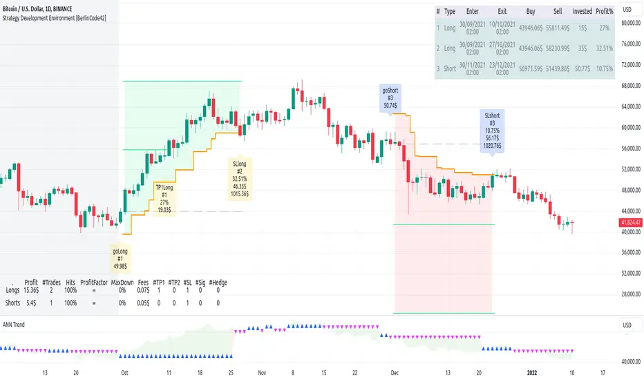
TTP VWAP BandThis indicator offers 20 VWAP bands and on-chart statistic data about the bands.
Features
- Longs and shorts
- Cherry-pick up to 5 bands for backtesting
- Plots 20 bands
- Step scale to increase deviation percentage on each band
- Period and timeframe selectors
- Band crosses: how many times a band was crossed (also percentage)
- Band bounces: how many times each band was pinched and bounced back (also percentage)
How to use:
1) Set the chart to 15 or 5 minute timeframe for higher backtesting accuracy
2) Select the first band deviation % (MIN Long VWAP % and MIN Short VWAP %), use a small number like 0.3 or 1.0 since the rest of the 20 bands will increase that amount later.
3) Select a step scale or leave it in 1 if you prefer same distance between all bands. Notice that if you use a value below 1 the bands will get closer to each other.
4) Observe the statistics and pay attention to how many times each of the bands are being crossed in percentage. This will later help you make decisions on when to enter and where to potentially put an SL.
Connect with your preferred backtester:
You can backtest a single or multiple bands at once. For example you could use the 7th band to enter a base order and later use crosses of the 4th band to enter safety orders. Any combination is possible!
Let's assume you decide that you will be backtesting only 1 band at the time as your single entry condition for your backtester.
Let's also assume that you want to use the 2nd band for long entries then do follow these steps:
- Set "Band 1 backtesting" to 2 so that it prints 1 every time the price crosses below the 2nd band.
- Leave the other Band backtesting band settings with a 0 so they stay disabled
- Add your backtester to the same chart and select "band 1 long signal"
- This signal will contain 1 every time your conditions are met

Unicorn QuantDeeply customizable trading algorithm with instant backtesting. It emulates real trading and displays all the actions it takes on the chart. For example, it shows when to enter or partially close a position, move Stop-Loss to breakeven, etc. The user can replicate these actions in their trading terminal in real time. The algorithm uses up to three Take-Profit levels, and a Stop-Loss level that can move in a trade to protect the floating profit.
The script can send real-time alerts to the user’s Email and to the cell phone via notifications in the TradingView app.
The indicator is designed to be used on all timeframes, including lower ones for intraday trading and scalping.
HOW TO USE
Set the Stop-Loss and up to three Take-Profit levels. Choose the rules for moving the Stop-Loss level in a trade. Adjust the sensitivity of the trading signals. And check the backtest result in the Instant Backtesting dashboard. If the performance of the strategy satisfies you, proceed with the forward testing or live trading.
When using this script, please, keep in mind that past results do not necessarily reflect future results and there are many factors that influence trading results.
FEATURES
Trading Signals
The feature calculates Buy and Sell signals for trend or swing trading. The user can change the Sensitivity parameter to control the frequency of the signals. This allows them to be adjusted for different markets and timeframes.
Position Manager
To make the Position Manager setup as easy as possible, the algorithm calculates Stop-Loss and Take-Profit levels in Average True Range (ATR) units. They are self-adjusting for any market and timeframe, since they account for its average volatility .
You don't have to worry about what market you are trading - Forex, Stocks, Crypto, etc. With the self-adjusting Stop-Loss and Take-Profit, you can find settings that work for one market and use the same numerical values as a starting point for a completely different market.
Instant Backtesting
After changing any settings, you can immediately see the performance of the strategy on the Instant Backtesting panel. Two metrics are displayed there - the percentage of profitable trades and the total return. This information, as well as the historical trades shown on the chart, will help you quickly and easily evaluate the settings.
SETTINGS
TRADING SIGNALS
Sensitivity - controls the sensitivity of the trading signals algorithm. It determines the frequency of the trading signals. The higher the value of this parameter, the less trading signals you get and the longer trends the algorithm tries to catch. The lower the sensitivity value, the more signals you receive. This can be useful if you want to profit from small price movements.
POSITION MANAGER
SL - sets the Stop-Loss level measured in ATR units.
TP1, TP2, TP3 - set the Take-Profit levels measured in the ATR units.
Close % at TP1, Close % at TP2, Close % at TP3 - set portions of the open position (as a percentage of the initial order size) to close at each of the TP levels.
At TP1 move SL to, At TP2 move SL to - set the rules for moving the Stop-Loss level in an open trade to protect the floating profit.
Show Open Position Dashboard - turns on/off a dashboard that shows the current Stop-Loss and Take-Profit levels for the open position.
BACKTESTING
Use Starting Date - turns on/off the starting date for the strategy and backtests. When off, all available historical data is used.
Starting Date - sets the starting date for the strategy and backtests.
Show Instant Backtesting Dashboard - turns on/off a dashboard that shows the current strategy performance: the percentage of profitable trades and total return.
Leverage - sets the leverage that the strategy uses.

Adaptive Trend SelectorThe Adaptive Trend Selector is a comprehensive trend-following tool designed to automatically identify the optimal moving average crossover strategy. It features adjustable parameters and an integrated backtester that delivers institutional-grade insights into the recommended strategy. The model continuously adapts to new data in real time by evaluating multiple moving average combinations, determining the best performing lengths, and presenting the backtest results in a clear, color-coded table that benchmarks performance against the buy-and-hold strategy.
At its core, the model systematically backtests a wide range of moving average combinations to identify the configuration that maximizes the selected optimization metric. Users can choose to optimize for absolute returns or risk-adjusted returns using the Sharpe, Sortino, or Calmar ratios. Alternatively, users can enable manual optimization to test custom fast and slow moving average lengths and view the corresponding backtest results. The label displays the Compounded Annual Growth Rate (CAGR) of the strategy, with the buy-and-hold CAGR in parentheses for comparison. The table presents the backtest results based on the fast and slow lengths displayed at the top:
Sharpe = CAGR per unit of standard deviation.
Sortino = CAGR per unit of downside deviation.
Calmar = CAGR relative to maximum drawdown.
Max DD = Largest peak-to-trough decline in value.
Beta (β) = Return sensitivity relative to buy-and-hold.
Alpha (α) = Excess annualized risk-adjusted returns.
Win Rate = Ratio of profitable trades to total trades.
Profit Factor = Total gross profit per unit of losses.
Expectancy = Average expected return per trade.
Trades/Year = Average number of trades per year.
This indicator is designed with flexibility in mind, enabling users to specify the start date of the backtesting period and the preferred moving average strategy. Supported strategies include the Exponential Moving Average (EMA), Simple Moving Average (SMA), Wilder’s Moving Average (RMA), Weighted Moving Average (WMA), and Volume-Weighted Moving Average (VWMA). To minimize overfitting, users can define constraints such as a minimum and maximum number of trades per year, as well as an optional optimization margin that prioritizes longer, more robust combinations by requiring shorter-length strategies to exceed this threshold. The table follows an intuitive color logic that enables quick performance comparison against buy-and-hold (B&H):
Sharpe = Green indicates better than B&H, while red indicates worse.
Sortino = Green indicates better than B&H, while red indicates worse.
Calmar = Green indicates better than B&H, while red indicates worse.
Max DD = Green indicates better than B&H, while red indicates worse.
Beta (β) = Green indicates better than B&H, while red indicates worse.
Alpha (α) = Green indicates above 0%, while red indicates below 0%.
Win Rate = Green indicates above 50%, while red indicates below 50%.
Profit Factor = Green indicates above 2, while red indicates below 1.
Expectancy = Green indicates above 0%, while red indicates below 0%.
In summary, the Adaptive Trend Selector is a powerful tool designed to help investors make data-driven decisions when selecting moving average crossover strategies. By optimizing for risk-adjusted returns, investors can confidently identify the best lengths using institutional-grade metrics. While results are based on the selected historical period, users should be mindful of potential overfitting, as past results may not persist under future market conditions. Since the model recalibrates to incorporate new data, the recommended lengths may evolve over time.

Great Expectations [LucF]Great Expectations helps traders answer the question: What is possible? It is a powerful question, yet exploration of the unknown always entails risk. A more complete set of questions better suited to traders could be:
What opportunity exists from any given point on a chart?
What portion of this opportunity can be realistically captured?
What risk will be incurred in trying to do so, and how long will it take?
Great Expectations is the result of an exploration of these questions. It is a trade simulator that generates visual and quantitative information to help strategy modelers visually identify and analyse areas of optimal expectation on charts, whether they are designing automated or discretionary strategies.
WARNING: Great Expectations is NOT an indicator that helps determine the current state of a market. It works by looking at points in the past from which the future is already known. It uses one definition of repainting extensively (i.e. it goes back in the past to print information that could not have been know at the time). Repainting understood that way is in fact almost all the indicator does! —albeit for what I hope is a noble cause. The indicator is of no use whatsoever in analyzing markets in real-time. If you do not understand what it does, please stay away!
This is an indicator—not a strategy that uses TradingView’s backtesting engine. It works by simulating trades, not unlike a backtest, but with the crucial difference that it assumes a trade (either long or short) is entered on all bars in the historic sample. It walks forward from each bar and determines possible outcomes, gathering individual trade statistics that in turn generate precious global statistics from all outcomes tested on the chart.
Great Expectations provides numbers summarizing trade results on all simulations run from the chart. Those numbers cannot be compared to backtest-produced numbers since all non-filtered bars are examined, even if an entry was taken on the bar immediately preceding the current one, which never happens in a backtest. This peculiarity does NOT invalidate Great Expectations calculations; it just entails that results be considered under a different light. Provided they are evaluated within the indicator’s context, they can be useful—sometimes even more than backtesting results, e.g. in evaluating the impact of parameter-fitting or variations in entry, exit or filtering strats.
Traders and strategy modelers are creatures of hope often suffering from blurred vision; my hope is that Great Expectations will help them appraise the validity of their setup and strat intuitions in a realistic fashion, preventing confirmation bias from obstructing perspective—and great expectations from turning into financial great deceptions.
USE CASES
You’ve identified what looks like a promising setup on other indicators. You load Great Expectations on the chart and evaluate if its high-expectation areas match locations where your setup’s conditions occur. Unless today is your lucky day, chances are the indicator will help you realize your setup is not as promising as you had hoped.
You want to get a rough estimate of the optimal trade duration for a chart and you don’t mind using the entry and exit strategies provided with the indicator. You use the trade length readouts of the indicator.
You’re experimenting with a new stop strategy and want to know how long it will keep you in trades, on average. You integrate your stop strategy in the indicator’s code and look at the average trade length it produces and the TST ratio to evaluate its performance.
You have put together your own entry and exit criteria and are looking for a filter that will help you improve backtesting results. You visually ascertain the suitability of your filter by looking at its results on the charts with great Expectations, to see if your filter is choosing its areas correctly.
You have a strategy that shows backtested trades on your chart. Great Expectations can help you evaluate how well your strategy is benefitting from high-opportunity areas while avoiding poor expectation spots.
You want more complete statistics on your set of strategies than what backtesting will provide. You use Great Expectations, knowing that it tests all bars in the sample that correspond to your criteria, as opposed to backtesting results which are limited to a subset of all possible entries.
You want to fool your friends into thinking you’ve designed the holy grail of indicators, something that identifies optimal opportunities on any chart; you show them the P&L cloud.
FEATURES
For one trade
At any given point on the chart, assuming a trade is entered there, Great Expectations shows you information specific to that trade simulation both on the chart and in the Data Window.
The chart can display:
the P & L Cloud which shows whether the trade ended profitably or not, and by how much,
the Opportunity & Risk Cloud which the maximum opportunity and risk the simulation encountered. When superimposed over the P & L cloud, you will see what I call the managed opportunity and risk, i.e the portion of maximum opportunity that was captured and the portion of the maximum risk that was incurred,
the target and if it was reached,
a background that uses a gradient to show different levels of trade length, P&L or how frequently the target was reached during simulation.
The Data Window displays more than 40 values on individual trades and global results. For any given trade you will know:
Entry/Exit levels, including slippage impact,
It’s outcome and duration,
P/L achieved,
The fraction of the maximum opportunity/risk managed by the trade.
For all trades
After going through all the possible trades on the chart, the indicator will provide you with a rare view of all outcomes expressed with the P&L cloud, which allows us to instantly see the most/least profitable areas of a chart using trade data as support, while also showing its relationship with the opportunity/risk encountered during the simulation. The difference between the two clouds is the managed opportunity and risk.
The Data Window will present you with numbers which we will go through later. Some of them are: average stop size, P/L, win rate, % opportunity managed, trade lengths for different types of trade outcomes and the TST (Target:Stop Travel) ratio.
Let’s see Great Expectations in action… and remember to open your Data Window!
INPUTS
Trade direction : You must first choose if you wish to look at long or short trades. Because of the way the indicator works and the amount of visual information on the chart, it is only practical to look at one type of trades at a time. The default is Longs.
Maximum trade Length (MaxL) : This is the maximum walk forward distance the simulator will go in analyzing outcomes from any given point in the past. It also determines the size of the dead zone among the chart’s last bars. A red background line identifies the beginning of the dead zone for which not enough bars have elapsed to analyze outcomes for the maximum trade length defined. If an ATR-based entry stop is used, that length is added to the wait time before beginning simulations, so that the first entry starts with a clean ATR value. On a sample of around 16000 bars, my tests show that the indicator runs into server errors at lengths of around 290, i.e. having completed ~4,6M simulation loop iterations. That is way too high a length anyways; 100 will usually be amply enough to ring out all the possibilities out of a simulation, and on shorter time frames, 30 can be enough. While making it unduly small will prevent simulations of expressing the market’s potential, the less you use, the faster the indicator will run. The default is 40.
Unrealized P&L base at End of Trade (EOT) : When a simulation ends and the trade is still open, we calculate unrealized P&L from an exit order executed from either the last in-trade stop on the previous bar, or the close of the last bar. You can readily see the impact of this selection on the chart, with the P&L cloud. The default is on the close.
Display : The check box besides the title does nothing.
Show target : Shows a green line displaying the trade’s target expressed as a multiple of X, i.e. the amplitude of the entry stop. I call this value “X” and use it as a unit to express profit and loss on a trade (some call it “R”). The line is highlighted for trades where the close reached the target during the trade, whether the trade ended in profit or loss. This is also where you specify the multiple of X you wish to use in calculating targets. The multiple is used even if targets are not displayed.
Show P&L Cloud : The cloud allows traders to see right away the profitable areas of the chart. The only line printed with the cloud is the “end of trade line” (EOT). The EOT line is the only way one can see the level where a trade ended on the chart (in the Data Window you can see it as the “Exit Fill” value). The EOT level for the trade determines if the trade ended in a profit or a loss. Its value represents one of the following:
- fill from order executed at close of bar where stop is breached during trade (which produces “Realized P/L”),
- simulation of a fill pseudo-fill at the user-defined EOT level (last close or stop level) if the trade runs its course through MaxL bars without getting stopped (producing Unrealized P/L).
The EOT line and the cloud fill print in green when the trade’s outcome is profitable and in red when it is not. If the trade was closed after breaching the stop, the line appears brighter.
Show Opportunity&Risk Cloud : Displays the maximum opportunity/risk that was present during the trade, i.e. the maximum and minimum prices reached.
Background Color Scheme : Allows you to choose between 3 different color schemes for the background gradients, to accommodate different types of chart background/candles. Select “None” if you don’t want a background.
Background source : Determines what value will be used to generate the different intensities of the gradient. You can choose trade length (brighter is shorter), Trade P&L (brighter is higher) or the number of times the target was reached during simulation (brighter is higher). The default is Trade Length.
Entry strat : The check box besides the title does nothing. The default strat is All bars, meaning a trade will be simulated from all bars not excluded by the filters where a MaxL bars future exists. For fun, I’ve included a pseudo-random entry strat (an indirect way of changing the seed is to vary the starting date of the simulation).
Show Filter State : Displays areas where the combination of filters you have selected are allowing entries. Filtering occurs as per your selection(s), whether the state is displayed or not. The effect of multiple selections is additive. The filters are:
1. Bar direction: Longs will only be entered if close>open and vice versa.
2. Rising Volume: Applies to both long and shorts.
3. Rising/falling MA of the length you choose over the number of bars you choose.
4. Custom indicator: You can feed your own filtering signal through this from another indicator. It must produce a signal of 1 to allow long entries and 0 to allow shorts.
Show Entry Stops :
1. Multiple of user-defined length ATR.
2. Fixed percentage.
3. Fixed value.
All entry stops are calculated using the entry fill price as a reference. The fill price is calculated from the current bar’s open, to which slippage is added if configured. This simulates the case where the strategy issued the entry signal on the previous bar for it to be executed at the next bar’s open.
The entry stop remains active until the in-trade stop becomes the more aggressive of the two stops. From then on, the entry stop will be ignored, unless a bar close breaches the in-trade stop, in which case the stop will be reset with a new entry stop and the process repeats.
Show In-trade stops : Displays in bright red the selected in-trade stop (be sure to read the note in this section about them).
1. ATR multiple: added/subtracted from the average of the two previous bars minimum/maximum of open/close.
2. A trailing stop with a deviation expressed as a multiple of entry stop (X).
3. A fixed percentage trailing stop.
Trailing stops deviations are measured from the highest/lowest high/low reached during the trade.
Note: There is a twist with the in-trade stops. It’s that for any given bar, its in-trade stop can hold multiple values, as each successive pass of the advancing simulation loops goes over it from a different entry points. What is printed is the stop from the loop that ended on that bar, which may have nothing to do with other instances of the trade’s in-trade stop for the same bar when visited from other starting points in previous simulations. There is just no practical way to print all stop values that were used for any given bar. While the printed entry stops are the actual ones used on each bar, the in-trade stops shown are merely the last instance used among many.
Include Slippage : if checked, slippage will be added/subtracted from order price to yield the fill price. Slippage is in percentage. If you choose to include slippage in the simulations, remember to adjust it by considering the liquidity of the markets and the time frame you’ll be analyzing.
Include Fees : if checked, fees will be subtracted/added to both realized an unrealized trade profits/losses. Fees are in percentage. The default fees work well for crypto markets but will need adjusting for others—especially in Forex. Remember to modify them accordingly as they can have a major impact on results. Both fees and slippage are included to remind us of their importance, even if the global numbers produced by the indicator are not representative of a real trading scenario composed of sequential trades.
Date Range filtering : the usual. Just note that the checkbox has to be selected for date filtering to activate.
DATA WINDOW
Most of the information produced by this indicator is made available in the Data Window, which you bring up by using the icon below the Watchlist and Alerts buttons at the right of the TV UI. Here’s what’s there.
Some of the information presented in the Data Window is standard trade data; other values are not so standard; e. g. the notions of managed opportunity and risk and Target:Stop Travel ratio. The interplay between all the values provided by Great Expectations is inherently complex, even for a static set of entry/filter/exit strats. During the constant updating which the habitual process of progressive refinement in building strategies that is the lot of strategy modelers entails, another level of complexity is no doubt added to the analysis of this indicator’s values. While I don’t want to sound like Wolfram presenting A New Kind of Science , I do believe that if you are a serious strategy modeler and spend the time required to get used to using all the information this indicator makes available, you may find it useful.
Trade Information
Entry Order : This is the open of the bar where simulation starts. We suppose that an entry signal was generated at the previous bar.
Entry Fill (including slip.) : The actual entry price, including slippage. This is the base price from which other values will be calculated.
Exit Order : When a stop is breached, an exit order is executed from the close of the bar that breached the stop. While there is no “In-trade stop” value included in the Data Window (other than the End of trade Stop previously discussed), this “Exit Order” value is how we can know the level where the trade was stopped during the simulation. The “Trade Length” value will then show the bar where the stop was breached.
Exit Fill (including slip.) : When the exit order is simulated, slippage is added to the order level to create the fill.
Chart: Target : This is the target calculated at the beginning of the simulation. This value also appear on the chart in teal. It is controlled by the multiple of X defined under the “Show Target” checkbox in the Inputs.
Chart: Entry Stop : This value also appears on the chart (the red dots under points where a trade was simulated). Its value is controlled by the Entry Strat chosen in the Inputs.
X (% Fill, including Fees) and X (currency) : This is the stop’s amplitude (Entry Fill – Entry Stop) + Fees. It represents the risk incurred upon entry and will be used to express P&L. We will show R expressed in both a percentage of the Entry Fill level (this value), and currency (the next value). This value represents the risk in the risk:reward ratio and is considered to be a unit of 1 so that RR can be expressed as a single value (i.e. “2” actually meaning “1:2”).
Trade Length : If trade was stopped, it’s the number of bars elapsed until then. The trade is then considered “Closed”. If the trade ends without being stopped (there is no profit-taking strat implemented, so the stop is the only exit strat), then the trade is “Open”, the length is MaxL and it will show in orange. Otherwise the value will print in green/red to reflect if the trade is winning/losing.
P&L (X) : The P&L of the trade, expressed as a multiple of X, which takes into account fees paid at entry and exit. Given our default target setting at 2 units of “X”, a trade that closes at its target will have produced a P&L of +2.0, i.e. twice the value of X (not counting fees paid at exit ). A trade that gets stopped late 50% further that the entry stop’s level will produce a P&L of -1.5X.
P&L (currency, including Fees) : same value as above, but expressed in currency.
Target first reached at bar : If price closed above the target during the trade (even if it occurs after the trade was stopped), this will show when. This value will be used in calculating our TST ratio.
Times Stop/Target reached in sim. : Includes all occurrences during the complete simulation loop.
Opportunity (X) : The highest/lowest price reached during a simulation, i.e. the maximum opportunity encountered, whether the trade was previously stopped or not, expressed as a multiple of X.
Risk (X) : The lowest/highest price reached during a simulation, i.e. the maximum risk encountered, whether the trade was previously stopped or not, expressed as a multiple of X.
Risk:Opportunity : The greater this ratio, the greater Opportunity is, compared to Risk.
Managed Opportunity (%) : The portion of Opportunity that was captured by the highest/low stop position, even if it occurred after a previous stop closed the trade.
Managed Risk (%) : The portion of risk that was protected by the lowest/highest stop position, even if it occurred after a previous stop closed the trade. When this value is greater than 100%, it means the trade’s stop is protecting more than the maximum risk, which is frequent. You will, however, never see close to those values for the Managed Opportunity value, since the stop would have to be higher than the Maximum opportunity. It is much easier to alleviate the risk than it is to lock in profits.
Managed Risk:Opportunity : The ratio of the two preceding values.
Managed Opp. vs. Risk : The Managed Opportunity minus the Managed Risk. When it is negative, which is most often is, it means your strat is protecting a greater portion of the risk than it captures opportunity.
Global Numbers
Win Rate(%) : Percentage of winning trades over all entries. Open trades are considered winning if their last stop/close (as per user selection) locks in profits.
Avg X%, Avg X (currency) : Averages of previously described values:.
Avg Profitability/Trade (APPT) : This measures expectation using: Average Profitability Per Trade = (Probability of Win × Average Win) − (Probability of Loss × Average Loss) . It quantifies the average expectation/trade, which RR alone can’t do, as the probabilities of each outcome (win/lose) must also be used to calculate expectancy. The APPT combine the RR with the win rate to yield the true expectancy of a strategy. In my usual way of expressing risk with X, APPT is the equivalent of the average P&L per trade expressed in X. An APPT of -1.5 means that we lose on average 1.5X/trade.
Equity (X), Equity (currency) : The cumulative result of all trade outcomes, expressed as a multiple of X. Multiplied by the Average X in currency, this yields the Equity in currency.
Risk:Opportunity, Managed Risk:Opportunity, Managed Opp. vs. Risk : The global values of the ones previously described.
Avg Trade Length (TL) : One of the most important values derived by going through all the simulations. Again, it is composed of either the length of stopped trades, or MaxL when the trade isn’t stopped (open). This value can help systems modelers shape the characteristics of the components they use to build their strategies.
Avg Closed Win TL and Avg Closed Lose TL : The average lengths of winning/losing trades that were stopped.
Target reached? Avg bars to Stop and Target reached? Avg bars to Target : For the trades where the target was reached at some point in the simulation, the number of bars to the first point where the stop was breached and where the target was reached, respectively. These two values are used to calculate the next value.
TST (Target:Stop Travel Ratio) : This tracks the ratio between the two preceding values (Bars to first stop/Bars to first target), but only for trades where the target was reached somewhere in the loop. A ratio of 2 means targets are reached twice as fast as stops.
The next values of this section are counts or percentages and are self-explanatory.
Chart Plots
Contains chart plots of values already describes.
NOTES
Optimization/Overfitting: There is a fine line between optimizing and overfitting. Tools like this indicator can lead unsuspecting modelers down a path of overfitting that often turns strategies into over-specialized beasts that do not perform elegantly when confronted to the real-world. Proven testing strategies like walk forward analysis will go a long way in helping modelers alleviate this risk.
Input tuning: Because the results generated by the indicator will vary with the parameters used in the active entry, filtering and exit strats, it’s important to realize that although it may be fun at first, just slapping the default settings on a chart and time frame will not yield optimal nor reliable results. While using ATR as often as possible (as I do in this indicator) is a good way to make strat parametrization adaptable, it is not a foolproof solution.
There is no data for the last MaxL bars of the chart, since not enough trade future has elapsed to run a simulation from MaxL bars back.
Modifying the code: I have tried to structure the code modularly, even if that entails a larger code base, so that you can adapt it to your needs. I’ve included a few token components in each of the placeholders designed for entry strategies, filters, entry stops and in-trade stops. This will hopefully make it easier to add your own. In the same spirit, I have also commented liberally.
You will find in the code many instances of standard trade management tasks that can be lifted to code TV strategies where, as I do in mine, you manage everything yourself and don’t rely on built-in Pine strategy functions to act on your trades.
Enjoy!
THANKS
To @scarf who showed me how plotchar() could be used to plot values without ruining scale.
To @glaz for the suggestion to include a Chandelier stop strat; I will.
To @simpelyfe for the idea of using an indicator input for the filters (if some day TV lets us use more than one, it will be useful in other modules of the indicator).
To @RicardoSantos for the random generator used in the random entry strat.
To all scripters publishing open source on TradingView; their code is the best way to learn.
To my trading buddies Irving and Bruno; who showed me way back how pro traders get it done.
Protervus Trading ToolkitHi Traders! Welcome to Protervus Trading Toolkit (PTT) , a comprehensive set of tools to help you building, backtesting, and even automating your strategy.
Important : the data and screenshots I publish are solely for presentation and explanation purposes and must not be intended as recommendations or guarantees. Please consider eventual backtesting results seen here as almost-random. My goal is not to provide ready-made strategies, signals, or infallible methods, but rather indicators and tools to help you focus on your own research and build a reliable trading plan based on discipline.
BUILD, BACKTEST, AUTOMATE
The first step is to link a chained indicator which will send Entry signals and, optionally, Exit signals: to integrate your own triggers with this toolkit, check out my tutorial and use this code as a template.
Then, in the Trading Settings you can set the Trading Mode (Full - Long and Short, Long only, or Short only) as well as Starting Capital, Drawdown Limit, Risk per Trade, Fees, and the date range in which trading will be enabled and backtested.
Go further by tweaking your strategy with built-in Take Profit and Stop Loss conditions, and keep it under control thanks to the Statistics Panel.
Trades will be shown on the chart, including TP\SL levels (according to the ones you enable) and per-trade statistics:
Tip: point the cursor over TP or SL icon to open the tooltip, showing additional details about the trade.
BUILT-IN CONDITIONS
Note: all conditions already account for fees.
Take Profit \ Stop Loss percentage
Take Profit or Stop at Loss when a fixed percentage is reached.
Limit \ Hard Stop: the trade will be considered closed when that specific price is reached - otherwise, the candle closing price will be used.
Trailing Take Profit
Trail the price and close the trade in profit when it reverses for the chosen percentage.
Engage and Disengage: activate trailing when the price is above the entry price for the chosen percentage, and de-activate it if price goes past the disengage percentage.
Safety TP: close the trade at Break-Even if the price sharply reverses from engaged area to BE level. A specific Alert is available in order to create a separate trigger with immediate effect.
Note: using TP Safety with an Engage % of zero might result in many early exits, so it is recommended to add some margin to Engage % to avoid that.
Exit \ Stop on Opposite Signal
Close the trade when another, contrary signal is received (e.g. close a Long position when a signal to go Short is received).
Exit \ Stop after X candles
Close the trade after X candles, as soon as the condition is met (e.g. for Take Profit condition, it will close the trade after X candles as soon as the trade is in profit).
Bind to TP \ SL: only validate the condition if the current PnL is above (TakeProfit cond.) or below (Stop Loss cond.) the specified percentage.
ATR Stop
Classic ATR Stop Loss.
Trailing ATR
Chase the price by the defined ratio and close the position when the candle closes past the ATR line.
Bind to TP \ SL: only validate the condition if the current PnL is above (TakeProfit cond.) or below (Stop Loss cond.) the specified percentage.
External Signal (sent from your indicator)
Close the position basing on your own triggers, defined in the chained indicator.
- Bind to TP \ SL: only validate the condition if the current PnL is above (TakeProfit cond.) or below (Stop Loss cond.) the specified percentage.
PANEL CUSTOMIZATION AND ADDITIONAL OPTIONS
A strategy name can be assigned in the settings and will show it at the top of the Statistics Panel, so you can better identify and label your tests and live instances.
The panel can be customized in terms of colors, text size and height. It can be also "split" in modular panels that will appear at the bottom of the chart.
It is also possible to show \ hide prices and live data labels as well as position and Break-Even levels. In some cases you will need to limit the display of those plots in order to avoid PineScript calculation issues.
If you limited the plots but you are checking very old trades, you can enable the Legacy position tracker to see basic markers for positions (position is active, and profit \ loss marker).
In the case you will be sending webhook alerts to a trading bot , "Position Alert Failover" will come in aid to prevent situations where the initial trade closing alert is either not sent or missed: it will keep sending the position closing signal for X candles.
PLUGINS
Thanks to the modular nature of PTT, plugins will eventually be available to provide additional features and extend functionalities even further. Make sure to keep an eye on updates.
CREATING ALERTS
To create alerts you must first select the PTT indicator from the "Condition" drop-down menu, then the whole list of available alerts will appear. When creating alerts, please make sure to set "Once Per Bar Close" for the normal conditions, and "Once Per Bar" for safety conditions (Limit and Hard Stop simulation, Trailing TP Safety Trigger).
Besides positions opening and closing alerts, you also have the option to add extra alerts for when a position is open or not open (e.g. Active Long position, No Long Position) - that might come handy when dealing with trading bots and automation tools. Also, as mentioned earlier, you have the chance to create a special alert as failover in order to repeat the closing alert.
TIPS AND RECOMMENDATIONS
Set Visual Order > Bring to front for PTT to avoid other indicators or candles covering up labels.
If you receive errors like "Referencing too many candles" or "Too many drawings", use the " Limit to last candles " function in the Settings panel to lower the number of candles.
If the Statistics Panel or labels are not appearing, and no errors are shown (red circled exclamation mark next to indicator's name), try changing any value in the settings to trigger a new calculation.
The Lowest Point in Trades refers to the maximum movement against your position. However, if the price never goes negative against the Entry level, it will be calculated from the Break-Even level.
Differently from TradingView's Strategy Tester, PTT calculates DrawDown from the Equity line (the starting balance).
Remember that Backtests only show past results, and although very useful to understand if your strategy makes sense, the market can completely change at any moment and ruin your dreams: make sure to avoid over-fitting (using very specific values) in your settings and to prefer more generic values in order to factor broader market situations.
After many successful backtests of your newly created strategy, let it run live without actually trading it for some time (paper trading), and see if it remains valid.
You can use multiple Conditions as safeguard. For example, main Stop condition can be Trailing ATR and secondary Stop condition can be Stop Loss % with Hard Stop, so you will be protected in case of sudden big price moves.
[Sextan] T-Step LSMA MTF BacktestLevel: 1
NOTE: This is a request by @scantor516 to backtest T-Step LSMA by alexgrover with my Sextan framework. You can backtest many of my indicators in minutes now! Of course,you can define your own indicator in the highlighted area in compliance with the uniform format, which guarantee when you use "Indicator on Indicator" function, it would not produce any error.
Courtesy of alexgrover for his T-Step LSMA
Background
Backtesting of technical indicators and strategies is the most common way to understand a quantitative strategy. However, the complicated configuration and adaptation work of backtesting many quantitative tools makes many traders who do not understand the code daunted. Moreover, although I have written a lot of strategies, I am still not very satisfied with the backtest configuration and writing efficiency. Therefore, I have been thinking about how to build a backtesting framework that can quickly and easily evaluate the backtesting performance of any indicator with a "long/short entry" indicator, that is, a "simple backtesting tool for dummies". The performance requirements should be stable, and the operation should be simple and convenient. It is best to "copy", "paste", and "a few mouse clicks" to complete the quick backtest and evaluation of a new indicator.
Luckily, I recently realized that TradingView provides an "Indicator on Indicator" feature, which is the perfect foundation for doing "hot swap" backtesting. My basic idea is to use a two-layer design. The first layer is the technical indicator signal source that needs to be embedded, which is only used to provide buy and sell signals of custom strategies; the second layer is the trading system, which is used to receive the output signals of the first layer, and filter the signals according to the agreed specifications. , Take Profit, Stop Loss, draw buy and sell signals and cost lines, define and send custom buy and sell alert messages to mobile phones, social software or trading interfaces. In general, this two-layer design is a flexible combination of "death and alive", which can meet the needs of most traders to quickly evaluate the performance of a certain technical indicator. The first layer here is flexible. Users can insert their own strategy codes according to my template, and they can draw buy and sell signals and output them to the second layer. The second layer is fixed, and the overall framework is solidified to ensure the stability and unity of the trading system. It is convenient to compare different or similar strategies under the same conditions. Finally, all trading signals are drawn on the chart, and the output strategy returns. test report.
The main function:
The first layer: "{Sextan} Your Indicator Source", the script provides a template for personalized strategy input, and the signal and definition interfaces ensure full compatibility with the second layer. Backtesting is performed stably in the backtesting framework of the layer. The first layer of this script is also relatively simple: enter your script in the highlighted custom script area, and after ensuring the final buy and sell signals long = bool condition, short = bool condition, the design of the first layer is considered complete. Input it into the PINE script editor of TradingView, save it and add it to the chart, you can see the pulse sequence in yellow (buy) and purple (sell) on the sub-picture, corresponding to the main picture, you can subjectively judge that the quality of the trading point of the strategy is good Bad.
The second layer: "{Sextan} PINEv4 Sextans Backtest Framework". This script is the standardized trading system strategy execution and alarm, used to generate the final report of the strategy backtest and some key indicators that I have customized that I find useful, such as: winning rate , Odds, Winning Surface, Kelly Ratio, Take Profit and Stop Loss Thresholds, Trading Frequency, etc. are evaluated according to the Kelly formula. To use the second layer, first load it into the TrainingView chart, no markers will appear on the chart, since you have not specified any strategy source signals, click on the gear-shaped setting next to the "{Sextan} PINEv4 Sextans BTFW" header button, you can open the backtest settings, the first item is to select your custom strategy source. Because we have added the strategy source to the chart in the previous step, you can easily find an option "{Sextan} Your Indicator Source: Signal" at the bottom of the list, this is the strategy source input we need, select and confirm , you can see various markers on the main graph, and quickly generate a backtesting profit graph and a list of backtesting reports. You can generate files and download the backtesting reports locally. You can also click the gear on the backtest chart interface to customize some conditions of the backtest, including: initial capital amount, currency type, percentage of each order placed, amount of pyramid additions, commission fees, slippage, etc. configuration. Note: The configuration in the interface dialog overrides the same configuration implemented by the code in the backtest script.
How to output charts:
The first layer: "{Sextan} Your Indicator Source", the output of this script is the pulse value of yellow and purple, yellow +1 means buy, purple -1 means sell.
The second layer: PINEv4 Sextans Backtest Framework". The output of this script is a bit complicated. After all, it is the entire trading system with a lot of information:
1. Blue and red arrows. The blue upward arrow indicates long position, the red downward arrow indicates short position, and the horizontal bar at the end of the purple arrow indicates take profit or stop loss exit.
2. Red and green lines. This is the holding cost line of the strategy, green represents the cost of holding a long position, and red represents the cost of holding a short position. The cost line is a continuous solid line and the price action is relatively close.
3. Green and yellow long take profit and stop loss area and green and yellow long take profit and stop loss fork. Once a long position is held, there is a conditional order for take profit and stop loss. The green horizontal line is the long take profit ratio line, and the yellow is the long stop loss ratio line; the green cross indicates the long take profit price, and the yellow cross indicates the long position. Stop loss price. It's worth noting that the prongs and wires don't necessarily go together. Because of the optimization of the algorithm, for a strong market, the take profit will occur after breaking the take profit line, and the profit will not be taken until the price falls.
4. The purple and red short take profit and stop loss area and the purple red short stop loss fork. Once a short position is held, there will be a take profit and stop loss conditional order, the red is the short take profit ratio line, and the purple is the short stop loss ratio line; the red cross indicates the short take profit price, and the purple cross indicates the short stop loss price.
5. In addition to the above signs, there are also text and numbers indicating the profit and loss values of long and short positions. "L" means long; "S" means short; "XL" means close long; "XS" means close short.
TradingView Strategy Tester Panel:
The overview graph is an intuitive graph that plots the blue (gain) and red (loss) curves of all backtest periods together, and notes: the absolute value and percentage of net profit, the number of all closed positions, the winning percentage, the profit factor, The maximum trading loss, the absolute value and ratio of the average trading profit and loss, and the average number of K-lines held in all trades.
Another is the performance summary. This is to display all long and short statistical indicators of backtesting in the form of a list, such as: net profit, gross profit, Sharpe ratio, maximum position, commission, times of profit and loss, etc.
Finally, the transaction list is a table indexed by the transaction serial number, showing the signal direction, date and time, price, profit and loss, accumulated profit and loss, maximum transaction profit, transaction loss and other values.
Remarks
Finally, I will explain that this is just the beginning of this model. I will continue to optimize the trading system of the second layer. Various optimization feedback and suggestions are welcome. For valuable feedback, I am willing to provide some L4/L5 technical indicators as rewards for free subscription rights.
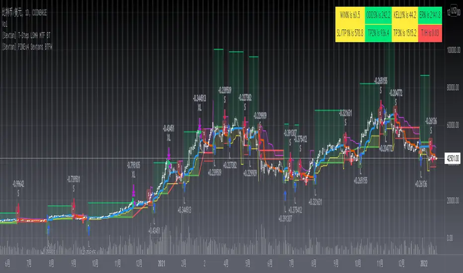
[Sextan] %R Trend Exhaustion BacktestLevel: 1
NOTE: This is a request by @upslidedown to backtest %R Trend Exhaustion by upslidedown with my Sextan framework. You can backtest many of my indicators in minutes now! Of course,you can define your own indicator in the highlighted area in compliance with the uniform format, which guarantee when you use "Indicator on Indicator" function, it would not produce any error.
Courtesy of upslidedown for his %R Trend Exhaustionindicator
Background
Backtesting of technical indicators and strategies is the most common way to understand a quantitative strategy. However, the complicated configuration and adaptation work of backtesting many quantitative tools makes many traders who do not understand the code daunted. Moreover, although I have written a lot of strategies, I am still not very satisfied with the backtest configuration and writing efficiency. Therefore, I have been thinking about how to build a backtesting framework that can quickly and easily evaluate the backtesting performance of any indicator with a "long/short entry" indicator, that is, a "simple backtesting tool for dummies". The performance requirements should be stable, and the operation should be simple and convenient. It is best to "copy", "paste", and "a few mouse clicks" to complete the quick backtest and evaluation of a new indicator.
Luckily, I recently realized that TradingView provides an "Indicator on Indicator" feature, which is the perfect foundation for doing "hot swap" backtesting. My basic idea is to use a two-layer design. The first layer is the technical indicator signal source that needs to be embedded, which is only used to provide buy and sell signals of custom strategies; the second layer is the trading system, which is used to receive the output signals of the first layer, and filter the signals according to the agreed specifications. , Take Profit, Stop Loss, draw buy and sell signals and cost lines, define and send custom buy and sell alert messages to mobile phones, social software or trading interfaces. In general, this two-layer design is a flexible combination of "death and alive", which can meet the needs of most traders to quickly evaluate the performance of a certain technical indicator. The first layer here is flexible. Users can insert their own strategy codes according to my template, and they can draw buy and sell signals and output them to the second layer. The second layer is fixed, and the overall framework is solidified to ensure the stability and unity of the trading system. It is convenient to compare different or similar strategies under the same conditions. Finally, all trading signals are drawn on the chart, and the output strategy returns. test report.
The main function:
The first layer: "{Sextan} Your Indicator Source", the script provides a template for personalized strategy input, and the signal and definition interfaces ensure full compatibility with the second layer. Backtesting is performed stably in the backtesting framework of the layer. The first layer of this script is also relatively simple: enter your script in the highlighted custom script area, and after ensuring the final buy and sell signals long = bool condition, short = bool condition, the design of the first layer is considered complete. Input it into the PINE script editor of TradingView, save it and add it to the chart, you can see the pulse sequence in yellow (buy) and purple (sell) on the sub-picture, corresponding to the main picture, you can subjectively judge that the quality of the trading point of the strategy is good Bad.
The second layer: "{Sextan} PINEv4 Sextans Backtest Framework". This script is the standardized trading system strategy execution and alarm, used to generate the final report of the strategy backtest and some key indicators that I have customized that I find useful, such as: winning rate , Odds, Winning Surface, Kelly Ratio, Take Profit and Stop Loss Thresholds, Trading Frequency, etc. are evaluated according to the Kelly formula. To use the second layer, first load it into the TrainingView chart, no markers will appear on the chart, since you have not specified any strategy source signals, click on the gear-shaped setting next to the "{Sextan} PINEv4 Sextans BTFW" header button, you can open the backtest settings, the first item is to select your custom strategy source. Because we have added the strategy source to the chart in the previous step, you can easily find an option "{Sextan} Your Indicator Source: Signal" at the bottom of the list, this is the strategy source input we need, select and confirm , you can see various markers on the main graph, and quickly generate a backtesting profit graph and a list of backtesting reports. You can generate files and download the backtesting reports locally. You can also click the gear on the backtest chart interface to customize some conditions of the backtest, including: initial capital amount, currency type, percentage of each order placed, amount of pyramid additions, commission fees, slippage, etc. configuration. Note: The configuration in the interface dialog overrides the same configuration implemented by the code in the backtest script.
How to output charts:
The first layer: "{Sextan} Your Indicator Source", the output of this script is the pulse value of yellow and purple, yellow +1 means buy, purple -1 means sell.
The second layer: PINEv4 Sextans Backtest Framework". The output of this script is a bit complicated. After all, it is the entire trading system with a lot of information:
1. Blue and red arrows. The blue upward arrow indicates long position, the red downward arrow indicates short position, and the horizontal bar at the end of the purple arrow indicates take profit or stop loss exit.
2. Red and green lines. This is the holding cost line of the strategy, green represents the cost of holding a long position, and red represents the cost of holding a short position. The cost line is a continuous solid line and the price action is relatively close.
3. Green and yellow long take profit and stop loss area and green and yellow long take profit and stop loss fork. Once a long position is held, there is a conditional order for take profit and stop loss. The green horizontal line is the long take profit ratio line, and the yellow is the long stop loss ratio line; the green cross indicates the long take profit price, and the yellow cross indicates the long position. Stop loss price. It's worth noting that the prongs and wires don't necessarily go together. Because of the optimization of the algorithm, for a strong market, the take profit will occur after breaking the take profit line, and the profit will not be taken until the price falls.
4. The purple and red short take profit and stop loss area and the purple red short stop loss fork. Once a short position is held, there will be a take profit and stop loss conditional order, the red is the short take profit ratio line, and the purple is the short stop loss ratio line; the red cross indicates the short take profit price, and the purple cross indicates the short stop loss price.
5. In addition to the above signs, there are also text and numbers indicating the profit and loss values of long and short positions. "L" means long; "S" means short; "XL" means close long; "XS" means close short.
TradingView Strategy Tester Panel:
The overview graph is an intuitive graph that plots the blue (gain) and red (loss) curves of all backtest periods together, and notes: the absolute value and percentage of net profit, the number of all closed positions, the winning percentage, the profit factor, The maximum trading loss, the absolute value and ratio of the average trading profit and loss, and the average number of K-lines held in all trades.
Another is the performance summary. This is to display all long and short statistical indicators of backtesting in the form of a list, such as: net profit, gross profit, Sharpe ratio, maximum position, commission, times of profit and loss, etc.
Finally, the transaction list is a table indexed by the transaction serial number, showing the signal direction, date and time, price, profit and loss, accumulated profit and loss, maximum transaction profit, transaction loss and other values.
Remarks
Finally, I will explain that this is just the beginning of this model. I will continue to optimize the trading system of the second layer. Various optimization feedback and suggestions are welcome. For valuable feedback, I am willing to provide some L4/L5 technical indicators as rewards for free subscription rights.

[Sextan] B-Xtrender BacktestLevel: 1
NOTE: This is a request by @scantor516 to backtest B-Xtrender @PuppyTherapy by QuantTherapy with my Sextan framework. You can backtest many of my indicators in minutes now! Of course,you can define your own indicator in the highlighted area in compliance with the uniform format, which guarantee when you use "Indicator on Indicator" function, it would not produce any error.
Courtesy of QuantTherapy for his B-Xtrender @PuppyTherapy
Background
Backtesting of technical indicators and strategies is the most common way to understand a quantitative strategy. However, the complicated configuration and adaptation work of backtesting many quantitative tools makes many traders who do not understand the code daunted. Moreover, although I have written a lot of strategies, I am still not very satisfied with the backtest configuration and writing efficiency. Therefore, I have been thinking about how to build a backtesting framework that can quickly and easily evaluate the backtesting performance of any indicator with a "long/short entry" indicator, that is, a "simple backtesting tool for dummies". The performance requirements should be stable, and the operation should be simple and convenient. It is best to "copy", "paste", and "a few mouse clicks" to complete the quick backtest and evaluation of a new indicator.
Luckily, I recently realized that TradingView provides an "Indicator on Indicator" feature, which is the perfect foundation for doing "hot swap" backtesting. My basic idea is to use a two-layer design. The first layer is the technical indicator signal source that needs to be embedded, which is only used to provide buy and sell signals of custom strategies; the second layer is the trading system, which is used to receive the output signals of the first layer, and filter the signals according to the agreed specifications. , Take Profit, Stop Loss, draw buy and sell signals and cost lines, define and send custom buy and sell alert messages to mobile phones, social software or trading interfaces. In general, this two-layer design is a flexible combination of "death and alive", which can meet the needs of most traders to quickly evaluate the performance of a certain technical indicator. The first layer here is flexible. Users can insert their own strategy codes according to my template, and they can draw buy and sell signals and output them to the second layer. The second layer is fixed, and the overall framework is solidified to ensure the stability and unity of the trading system. It is convenient to compare different or similar strategies under the same conditions. Finally, all trading signals are drawn on the chart, and the output strategy returns. test report.
The main function:
The first layer: "{Sextan} Your Indicator Source", the script provides a template for personalized strategy input, and the signal and definition interfaces ensure full compatibility with the second layer. Backtesting is performed stably in the backtesting framework of the layer. The first layer of this script is also relatively simple: enter your script in the highlighted custom script area, and after ensuring the final buy and sell signals long = bool condition, short = bool condition, the design of the first layer is considered complete. Input it into the PINE script editor of TradingView, save it and add it to the chart, you can see the pulse sequence in yellow (buy) and purple (sell) on the sub-picture, corresponding to the main picture, you can subjectively judge that the quality of the trading point of the strategy is good Bad.
The second layer: "{Sextan} PINEv4 Sextans Backtest Framework". This script is the standardized trading system strategy execution and alarm, used to generate the final report of the strategy backtest and some key indicators that I have customized that I find useful, such as: winning rate , Odds, Winning Surface, Kelly Ratio, Take Profit and Stop Loss Thresholds, Trading Frequency, etc. are evaluated according to the Kelly formula. To use the second layer, first load it into the TrainingView chart, no markers will appear on the chart, since you have not specified any strategy source signals, click on the gear-shaped setting next to the "{Sextan} PINEv4 Sextans BTFW" header button, you can open the backtest settings, the first item is to select your custom strategy source. Because we have added the strategy source to the chart in the previous step, you can easily find an option "{Sextan} Your Indicator Source: Signal" at the bottom of the list, this is the strategy source input we need, select and confirm , you can see various markers on the main graph, and quickly generate a backtesting profit graph and a list of backtesting reports. You can generate files and download the backtesting reports locally. You can also click the gear on the backtest chart interface to customize some conditions of the backtest, including: initial capital amount, currency type, percentage of each order placed, amount of pyramid additions, commission fees, slippage, etc. configuration. Note: The configuration in the interface dialog overrides the same configuration implemented by the code in the backtest script.
How to output charts:
The first layer: "{Sextan} Your Indicator Source", the output of this script is the pulse value of yellow and purple, yellow +1 means buy, purple -1 means sell.
The second layer: PINEv4 Sextans Backtest Framework". The output of this script is a bit complicated. After all, it is the entire trading system with a lot of information:
1. Blue and red arrows. The blue upward arrow indicates long position, the red downward arrow indicates short position, and the horizontal bar at the end of the purple arrow indicates take profit or stop loss exit.
2. Red and green lines. This is the holding cost line of the strategy, green represents the cost of holding a long position, and red represents the cost of holding a short position. The cost line is a continuous solid line and the price action is relatively close.
3. Green and yellow long take profit and stop loss area and green and yellow long take profit and stop loss fork. Once a long position is held, there is a conditional order for take profit and stop loss. The green horizontal line is the long take profit ratio line, and the yellow is the long stop loss ratio line; the green cross indicates the long take profit price, and the yellow cross indicates the long position. Stop loss price. It's worth noting that the prongs and wires don't necessarily go together. Because of the optimization of the algorithm, for a strong market, the take profit will occur after breaking the take profit line, and the profit will not be taken until the price falls.
4. The purple and red short take profit and stop loss area and the purple red short stop loss fork. Once a short position is held, there will be a take profit and stop loss conditional order, the red is the short take profit ratio line, and the purple is the short stop loss ratio line; the red cross indicates the short take profit price, and the purple cross indicates the short stop loss price.
5. In addition to the above signs, there are also text and numbers indicating the profit and loss values of long and short positions. "L" means long; "S" means short; "XL" means close long; "XS" means close short.
TradingView Strategy Tester Panel:
The overview graph is an intuitive graph that plots the blue (gain) and red (loss) curves of all backtest periods together, and notes: the absolute value and percentage of net profit, the number of all closed positions, the winning percentage, the profit factor, The maximum trading loss, the absolute value and ratio of the average trading profit and loss, and the average number of K-lines held in all trades.
Another is the performance summary. This is to display all long and short statistical indicators of backtesting in the form of a list, such as: net profit, gross profit, Sharpe ratio, maximum position, commission, times of profit and loss, etc.
Finally, the transaction list is a table indexed by the transaction serial number, showing the signal direction, date and time, price, profit and loss, accumulated profit and loss, maximum transaction profit, transaction loss and other values.
Remarks
Finally, I will explain that this is just the beginning of this model. I will continue to optimize the trading system of the second layer. Various optimization feedback and suggestions are welcome. For valuable feedback, I am willing to provide some L4/L5 technical indicators as rewards for free subscription rights.
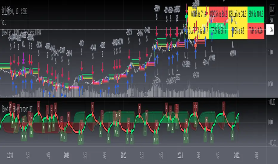
[Sextan] Haos Vieual BacktestLevel: 1
NOTE: This is a request by @scantor516 to backtest Haos Visual @PuppyTherapy by QuantTherapy with my Sextan framework. You can backtest many of my indicators in minutes now! Of course,you can define your own indicator in the highlighted area in compliance with the uniform format, which guarantee when you use "Indicator on Indicator" function, it would not produce any error.
Courtesy of QuantTherapy for his Haos Visual @PuppyTherapy
Background
Backtesting of technical indicators and strategies is the most common way to understand a quantitative strategy. However, the complicated configuration and adaptation work of backtesting many quantitative tools makes many traders who do not understand the code daunted. Moreover, although I have written a lot of strategies, I am still not very satisfied with the backtest configuration and writing efficiency. Therefore, I have been thinking about how to build a backtesting framework that can quickly and easily evaluate the backtesting performance of any indicator with a "long/short entry" indicator, that is, a "simple backtesting tool for dummies". The performance requirements should be stable, and the operation should be simple and convenient. It is best to "copy", "paste", and "a few mouse clicks" to complete the quick backtest and evaluation of a new indicator.
Luckily, I recently realized that TradingView provides an "Indicator on Indicator" feature, which is the perfect foundation for doing "hot swap" backtesting. My basic idea is to use a two-layer design. The first layer is the technical indicator signal source that needs to be embedded, which is only used to provide buy and sell signals of custom strategies; the second layer is the trading system, which is used to receive the output signals of the first layer, and filter the signals according to the agreed specifications. , Take Profit, Stop Loss, draw buy and sell signals and cost lines, define and send custom buy and sell alert messages to mobile phones, social software or trading interfaces. In general, this two-layer design is a flexible combination of "death and alive", which can meet the needs of most traders to quickly evaluate the performance of a certain technical indicator. The first layer here is flexible. Users can insert their own strategy codes according to my template, and they can draw buy and sell signals and output them to the second layer. The second layer is fixed, and the overall framework is solidified to ensure the stability and unity of the trading system. It is convenient to compare different or similar strategies under the same conditions. Finally, all trading signals are drawn on the chart, and the output strategy returns. test report.
The main function:
The first layer: "{Sextan} Your Indicator Source", the script provides a template for personalized strategy input, and the signal and definition interfaces ensure full compatibility with the second layer. Backtesting is performed stably in the backtesting framework of the layer. The first layer of this script is also relatively simple: enter your script in the highlighted custom script area, and after ensuring the final buy and sell signals long = bool condition, short = bool condition, the design of the first layer is considered complete. Input it into the PINE script editor of TradingView, save it and add it to the chart, you can see the pulse sequence in yellow (buy) and purple (sell) on the sub-picture, corresponding to the main picture, you can subjectively judge that the quality of the trading point of the strategy is good Bad.
The second layer: "{Sextan} PINEv4 Sextans Backtest Framework". This script is the standardized trading system strategy execution and alarm, used to generate the final report of the strategy backtest and some key indicators that I have customized that I find useful, such as: winning rate , Odds, Winning Surface, Kelly Ratio, Take Profit and Stop Loss Thresholds, Trading Frequency, etc. are evaluated according to the Kelly formula. To use the second layer, first load it into the TrainingView chart, no markers will appear on the chart, since you have not specified any strategy source signals, click on the gear-shaped setting next to the "{Sextan} PINEv4 Sextans BTFW" header button, you can open the backtest settings, the first item is to select your custom strategy source. Because we have added the strategy source to the chart in the previous step, you can easily find an option "{Sextan} Your Indicator Source: Signal" at the bottom of the list, this is the strategy source input we need, select and confirm , you can see various markers on the main graph, and quickly generate a backtesting profit graph and a list of backtesting reports. You can generate files and download the backtesting reports locally. You can also click the gear on the backtest chart interface to customize some conditions of the backtest, including: initial capital amount, currency type, percentage of each order placed, amount of pyramid additions, commission fees, slippage, etc. configuration. Note: The configuration in the interface dialog overrides the same configuration implemented by the code in the backtest script.
How to output charts:
The first layer: "{Sextan} Your Indicator Source", the output of this script is the pulse value of yellow and purple, yellow +1 means buy, purple -1 means sell.
The second layer: PINEv4 Sextans Backtest Framework". The output of this script is a bit complicated. After all, it is the entire trading system with a lot of information:
1. Blue and red arrows. The blue upward arrow indicates long position, the red downward arrow indicates short position, and the horizontal bar at the end of the purple arrow indicates take profit or stop loss exit.
2. Red and green lines. This is the holding cost line of the strategy, green represents the cost of holding a long position, and red represents the cost of holding a short position. The cost line is a continuous solid line and the price action is relatively close.
3. Green and yellow long take profit and stop loss area and green and yellow long take profit and stop loss fork. Once a long position is held, there is a conditional order for take profit and stop loss. The green horizontal line is the long take profit ratio line, and the yellow is the long stop loss ratio line; the green cross indicates the long take profit price, and the yellow cross indicates the long position. Stop loss price. It's worth noting that the prongs and wires don't necessarily go together. Because of the optimization of the algorithm, for a strong market, the take profit will occur after breaking the take profit line, and the profit will not be taken until the price falls.
4. The purple and red short take profit and stop loss area and the purple red short stop loss fork. Once a short position is held, there will be a take profit and stop loss conditional order, the red is the short take profit ratio line, and the purple is the short stop loss ratio line; the red cross indicates the short take profit price, and the purple cross indicates the short stop loss price.
5. In addition to the above signs, there are also text and numbers indicating the profit and loss values of long and short positions. "L" means long; "S" means short; "XL" means close long; "XS" means close short.
TradingView Strategy Tester Panel:
The overview graph is an intuitive graph that plots the blue (gain) and red (loss) curves of all backtest periods together, and notes: the absolute value and percentage of net profit, the number of all closed positions, the winning percentage, the profit factor, The maximum trading loss, the absolute value and ratio of the average trading profit and loss, and the average number of K-lines held in all trades.
Another is the performance summary. This is to display all long and short statistical indicators of backtesting in the form of a list, such as: net profit, gross profit, Sharpe ratio, maximum position, commission, times of profit and loss, etc.
Finally, the transaction list is a table indexed by the transaction serial number, showing the signal direction, date and time, price, profit and loss, accumulated profit and loss, maximum transaction profit, transaction loss and other values.
Remarks
Finally, I will explain that this is just the beginning of this model. I will continue to optimize the trading system of the second layer. Various optimization feedback and suggestions are welcome. For valuable feedback, I am willing to provide some L4/L5 technical indicators as rewards for free subscription rights.

[Sextan] Delta-RSI Oscillator BacktestLevel: 1
NOTE: This is a request by @scantor516 to backtest Delta-RSI Oscillator by tbiktag with my Sextan framework. You can backtest many of my indicators in minutes now! Of course,you can define your own indicator in the highlighted area in compliance with the uniform format, which guarantee when you use "Indicator on Indicator" function, it would not produce any error.
Courtesy of tbiktag for his Delta-RSI Oscillator Strategy
Background
Backtesting of technical indicators and strategies is the most common way to understand a quantitative strategy. However, the complicated configuration and adaptation work of backtesting many quantitative tools makes many traders who do not understand the code daunted. Moreover, although I have written a lot of strategies, I am still not very satisfied with the backtest configuration and writing efficiency. Therefore, I have been thinking about how to build a backtesting framework that can quickly and easily evaluate the backtesting performance of any indicator with a "long/short entry" indicator, that is, a "simple backtesting tool for dummies". The performance requirements should be stable, and the operation should be simple and convenient. It is best to "copy", "paste", and "a few mouse clicks" to complete the quick backtest and evaluation of a new indicator.
Luckily, I recently realized that TradingView provides an "Indicator on Indicator" feature, which is the perfect foundation for doing "hot swap" backtesting. My basic idea is to use a two-layer design. The first layer is the technical indicator signal source that needs to be embedded, which is only used to provide buy and sell signals of custom strategies; the second layer is the trading system, which is used to receive the output signals of the first layer, and filter the signals according to the agreed specifications. , Take Profit, Stop Loss, draw buy and sell signals and cost lines, define and send custom buy and sell alert messages to mobile phones, social software or trading interfaces. In general, this two-layer design is a flexible combination of "death and alive", which can meet the needs of most traders to quickly evaluate the performance of a certain technical indicator. The first layer here is flexible. Users can insert their own strategy codes according to my template, and they can draw buy and sell signals and output them to the second layer. The second layer is fixed, and the overall framework is solidified to ensure the stability and unity of the trading system. It is convenient to compare different or similar strategies under the same conditions. Finally, all trading signals are drawn on the chart, and the output strategy returns. test report.
The main function:
The first layer: "{Sextan} Your Indicator Source", the script provides a template for personalized strategy input, and the signal and definition interfaces ensure full compatibility with the second layer. Backtesting is performed stably in the backtesting framework of the layer. The first layer of this script is also relatively simple: enter your script in the highlighted custom script area, and after ensuring the final buy and sell signals long = bool condition, short = bool condition, the design of the first layer is considered complete. Input it into the PINE script editor of TradingView, save it and add it to the chart, you can see the pulse sequence in yellow (buy) and purple (sell) on the sub-picture, corresponding to the main picture, you can subjectively judge that the quality of the trading point of the strategy is good Bad.
The second layer: "{Sextan} PINEv4 Sextans Backtest Framework". This script is the standardized trading system strategy execution and alarm, used to generate the final report of the strategy backtest and some key indicators that I have customized that I find useful, such as: winning rate , Odds, Winning Surface, Kelly Ratio, Take Profit and Stop Loss Thresholds, Trading Frequency, etc. are evaluated according to the Kelly formula. To use the second layer, first load it into the TrainingView chart, no markers will appear on the chart, since you have not specified any strategy source signals, click on the gear-shaped setting next to the "{Sextan} PINEv4 Sextans BTFW" header button, you can open the backtest settings, the first item is to select your custom strategy source. Because we have added the strategy source to the chart in the previous step, you can easily find an option "{Sextan} Your Indicator Source: Signal" at the bottom of the list, this is the strategy source input we need, select and confirm , you can see various markers on the main graph, and quickly generate a backtesting profit graph and a list of backtesting reports. You can generate files and download the backtesting reports locally. You can also click the gear on the backtest chart interface to customize some conditions of the backtest, including: initial capital amount, currency type, percentage of each order placed, amount of pyramid additions, commission fees, slippage, etc. configuration. Note: The configuration in the interface dialog overrides the same configuration implemented by the code in the backtest script.
How to output charts:
The first layer: "{Sextan} Your Indicator Source", the output of this script is the pulse value of yellow and purple, yellow +1 means buy, purple -1 means sell.
The second layer: PINEv4 Sextans Backtest Framework". The output of this script is a bit complicated. After all, it is the entire trading system with a lot of information:
1. Blue and red arrows. The blue upward arrow indicates long position, the red downward arrow indicates short position, and the horizontal bar at the end of the purple arrow indicates take profit or stop loss exit.
2. Red and green lines. This is the holding cost line of the strategy, green represents the cost of holding a long position, and red represents the cost of holding a short position. The cost line is a continuous solid line and the price action is relatively close.
3. Green and yellow long take profit and stop loss area and green and yellow long take profit and stop loss fork. Once a long position is held, there is a conditional order for take profit and stop loss. The green horizontal line is the long take profit ratio line, and the yellow is the long stop loss ratio line; the green cross indicates the long take profit price, and the yellow cross indicates the long position. Stop loss price. It's worth noting that the prongs and wires don't necessarily go together. Because of the optimization of the algorithm, for a strong market, the take profit will occur after breaking the take profit line, and the profit will not be taken until the price falls.
4. The purple and red short take profit and stop loss area and the purple red short stop loss fork. Once a short position is held, there will be a take profit and stop loss conditional order, the red is the short take profit ratio line, and the purple is the short stop loss ratio line; the red cross indicates the short take profit price, and the purple cross indicates the short stop loss price.
5. In addition to the above signs, there are also text and numbers indicating the profit and loss values of long and short positions. "L" means long; "S" means short; "XL" means close long; "XS" means close short.
TradingView Strategy Tester Panel:
The overview graph is an intuitive graph that plots the blue (gain) and red (loss) curves of all backtest periods together, and notes: the absolute value and percentage of net profit, the number of all closed positions, the winning percentage, the profit factor, The maximum trading loss, the absolute value and ratio of the average trading profit and loss, and the average number of K-lines held in all trades.
Another is the performance summary. This is to display all long and short statistical indicators of backtesting in the form of a list, such as: net profit, gross profit, Sharpe ratio, maximum position, commission, times of profit and loss, etc.
Finally, the transaction list is a table indexed by the transaction serial number, showing the signal direction, date and time, price, profit and loss, accumulated profit and loss, maximum transaction profit, transaction loss and other values.
Remarks
Finally, I will explain that this is just the beginning of this model. I will continue to optimize the trading system of the second layer. Various optimization feedback and suggestions are welcome. For valuable feedback, I am willing to provide some L4/L5 technical indicators as rewards for free subscription rights.
