Ichimoku ACE ClubA. Overview:
This script is a custom implementation of the Ichimoku Cloud indicator for the TradingView platform, built using Pine Script version 4. It adds additional features like custom "Knife" lines and circle markers for specific data points. The indicator overlays on the chart and plots various elements of the Ichimoku system, including the Tenkan, Kijun, Chikou, and Kumo Cloud.
B. Inputs:
1. Tenkan (TS): This is the short-term moving average line (default period: 9).
2. Kijun (KJ): This is the medium-term moving average line (default period: 17).
3. Knife1 (K1): This line is based on a longer-term moving average (default period: 65).
4. Knife2 (K2): Another long-term moving average line (default period: 129).
5. Chikou Displacement (Chikou_Disp): The Chikou Span is plotted with a delay of 26 periods by default.
6. Displacement (disp): Determines the horizontal shift of the Kumo cloud.
C. Functions:
- `donchian(len)`: This function calculates the Donchian channel, which is the average of the highest high and the lowest low over the given period (len).
- `mf(len, offset)`: This function calculates the highest high and the lowest low over the given period, with an offset applied.
D. Plots:
1. Tenkan, Kijun, Knife1, and Knife2: These are plotted as lines with different colors and thicknesses.
- Tenkan is blue.
- Kijun is red.
- Knife1 is yellow.
- Knife2 is orange.
2. Chikou Span: This is plotted with a displacement and shown in purple.
3. Kumo Cloud: The cloud is formed by plotting two lines, Span A (green) and Span B (magenta), which represent the top and bottom of the cloud, respectively. The space between these lines is filled with a semi-transparent color, either green or magenta, depending on the relative position of the two spans.
E. Circle Markers:
- Additional circle markers are plotted for each of the Tenkan, Kijun, Knife1, and Knife2 lines at various offsets, helping to visualize the historical data points for each of these indicators. These circles are color-coded according to the line they correspond to.
F. Customization:
- The indicator allows customization of the lengths (periods) for Tenkan, Kijun, Knife1, Knife2, and other components via the script's input fields.
G. Conclusion:
This Ichimoku-based indicator provides a detailed view of the market's trend strength and direction. It offers a unique addition with the Knife lines and visual aids like circle markers for specific periods, which helps traders make better-informed decisions based on Ichimoku analysis.
---
You can modify the parameters such as `TS`, `KJ`, `K1`, `K2`, and `disp` according to your trading preferences. The colors and line thicknesses can also be adjusted for better visual representation.
"donchian"に関するスクリプトを検索

supertrendLibrary "supertrend"
supertrend : Library dedicated to different variations of supertrend
supertrend_atr(length, multiplier, atrMaType, source, highSource, lowSource, waitForClose, delayed)
supertrend_atr: Simple supertrend based on atr but also takes into consideration of custom MA Type, sources
Parameters:
length (simple int) : : ATR Length
multiplier (simple float) : : ATR Multiplier
atrMaType (simple string) : : Moving Average type for ATR calculation. This can be sma, ema, hma, rma, wma, vwma, swma
source (float) : : Default is close. Can Chose custom source
highSource (float) : : Default is high. Can also use close price for both high and low source
lowSource (float) : : Default is low. Can also use close price for both high and low source
waitForClose (simple bool) : : Considers source for direction change crossover if checked. Else, uses highSource and lowSource.
delayed (simple bool) : : if set to true lags supertrend atr stop based on target levels.
Returns: dir : Supertrend direction
supertrend : BuyStop if direction is 1 else SellStop
supertrend_bands(bandType, maType, length, multiplier, source, highSource, lowSource, waitForClose, useTrueRange, useAlternateSource, alternateSource, sticky)
supertrend_bands: Simple supertrend based on atr but also takes into consideration of custom MA Type, sources
Parameters:
bandType (simple string) : : Type of band used - can be bb, kc or dc
maType (simple string) : : Moving Average type for Bands. This can be sma, ema, hma, rma, wma, vwma, swma
length (simple int) : : Band Length
multiplier (float) : : Std deviation or ATR multiplier for Bollinger Bands and Keltner Channel
source (float) : : Default is close. Can Chose custom source
highSource (float) : : Default is high. Can also use close price for both high and low source
lowSource (float) : : Default is low. Can also use close price for both high and low source
waitForClose (simple bool) : : Considers source for direction change crossover if checked. Else, uses highSource and lowSource.
useTrueRange (simple bool) : : Used for Keltner channel. If set to false, then high-low is used as range instead of true range
useAlternateSource (simple bool) : - Custom source is used for Donchian Chanbel only if useAlternateSource is set to true
alternateSource (float) : - Custom source for Donchian channel
sticky (simple bool) : : if set to true borders change only when price is beyond borders.
Returns: dir : Supertrend direction
supertrend : BuyStop if direction is 1 else SellStop
supertrend_zigzag(length, history, useAlternativeSource, alternativeSource, source, highSource, lowSource, waitForClose, atrlength, multiplier, atrMaType)
supertrend_zigzag: Zigzag pivot based supertrend
Parameters:
length (simple int) : : Zigzag Length
history (simple int) : : number of historical pivots to consider
useAlternativeSource (simple bool)
alternativeSource (float)
source (float) : : Default is close. Can Chose custom source
highSource (float) : : Default is high. Can also use close price for both high and low source
lowSource (float) : : Default is low. Can also use close price for both high and low source
waitForClose (simple bool) : : Considers source for direction change crossover if checked. Else, uses highSource and lowSource.
atrlength (simple int) : : ATR Length
multiplier (simple float) : : ATR Multiplier
atrMaType (simple string) : : Moving Average type for ATR calculation. This can be sma, ema, hma, rma, wma, vwma, swma
Returns: dir : Supertrend direction
supertrend : BuyStop if direction is 1 else SellStop
zupertrend(length, history, useAlternativeSource, alternativeSource, source, highSource, lowSource, waitForClose, atrlength, multiplier, atrMaType)
zupertrend: Zigzag pivot based supertrend
Parameters:
length (simple int) : : Zigzag Length
history (simple int) : : number of historical pivots to consider
useAlternativeSource (simple bool)
alternativeSource (float)
source (float) : : Default is close. Can Chose custom source
highSource (float) : : Default is high. Can also use close price for both high and low source
lowSource (float) : : Default is low. Can also use close price for both high and low source
waitForClose (simple bool) : : Considers source for direction change crossover if checked. Else, uses highSource and lowSource.
atrlength (simple int) : : ATR Length
multiplier (simple float) : : ATR Multiplier
atrMaType (simple string) : : Moving Average type for ATR calculation. This can be sma, ema, hma, rma, wma, vwma, swma
Returns: dir : Supertrend direction
supertrend : BuyStop if direction is 1 else SellStop
zsupertrend(zigzagpivots, history, source, highSource, lowSource, waitForClose, atrMaType, atrlength, multiplier)
zsupertrend: Same as zigzag supertrend. But, works on already calculated array rather than Calculating fresh zigzag
Parameters:
zigzagpivots (array) : : Precalculated zigzag pivots
history (simple int) : : number of historical pivots to consider
source (float) : : Default is close. Can Chose custom source
highSource (float) : : Default is high. Can also use close price for both high and low source
lowSource (float) : : Default is low. Can also use close price for both high and low source
waitForClose (simple bool) : : Considers source for direction change crossover if checked. Else, uses highSource and lowSource.
atrMaType (simple string) : : Moving Average type for ATR calculation. This can be sma, ema, hma, rma, wma, vwma, swma
atrlength (simple int) : : ATR Length
multiplier (simple float) : : ATR Multiplier
Returns: dir : Supertrend direction
supertrend : BuyStop if direction is 1 else SellStop

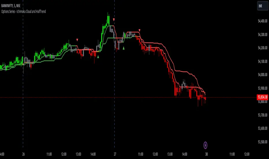
Options Series - Ichimoku Cloud and HalfTrend
The provided script combines two powerful technical indicators, Ichimoku Cloud and HalfTrend, to create a hybrid trading tool. Here's an analysis of the key components and how they work together:
Ichimoku Cloud and HalfTrend
⭐ 1. Indicator Title and Settings:
The script sets the title as "Options Series - Ichimoku Cloud and HalfTrend" and uses the overlay=true option to display the indicators directly on the price chart.
⭐ 2. Color Definitions:
Several colors are defined for later use:
Green and Red for different types of candles and signals.
Fluorescent Colors for highlighting significant trends or changes in market conditions.
⭐ 3. Ichimoku Cloud Setup:
The Ichimoku Cloud is a comprehensive indicator used to identify support, resistance, and trend direction. Here’s how the script configures it:
Conversion Periods, Base Periods, Lagging Span 2 Periods, and Displacement are customizable via input options, giving flexibility to adjust Ichimoku settings based on different market conditions.
The function donchian(len) calculates the Donchian Channel average, which is used to define the Conversion Line and Base Line. The crossover of these lines is crucial in determining bullish or bearish trends.
Color Logic for Kijun Cross: If the Conversion Line is above the Base Line, the trend is bullish (green color), while a bearish trend is indicated by red. A neutral condition is marked with orange.
⭐ 4. HalfTrend Indicator Setup:
The HalfTrend indicator detects trend reversals based on high/low price deviations from a moving average:
Amplitude and Channel Deviation inputs allow users to control the sensitivity of the indicator.
showArrows and showChannels toggle the display of buy/sell arrows and trend channels.
maxLowPrice and minHighPrice variables are initialized to track significant high/low points during the trend, used to confirm trend reversals.
⭐ 5. ATR and Trend Calculations:
The Average True Range (ATR) is used to calculate the volatility-based channels. The script calculates atr2 and uses this to create atrHigh and atrLow for plotting the channel.
The trend detection logic is as follows:
When the trend is upward, the script seeks confirmation by comparing the high moving average with previous lows, signaling a continuation of the uptrend if it holds.
Conversely, a downtrend is confirmed when the low moving average exceeds previous highs.
⭐ 6. Customized Candle Coloring:
A custom color scheme is applied to candles based on a combination of trend direction and Ichimoku Cloud signals:
GreenFluorescent for strong bullish conditions where price is above the HalfTrend line, and the Conversion Line is above the Base Line.
RedFluorescent for strong bearish conditions, with price below the HalfTrend line and Conversion Line below the Base Line.
Gray for neutral or indecisive conditions.
⭐ 7. Plots and Shapes:
The script plots various elements:
HalfTrend Line: The main trendline is plotted in either green (buy) or red (sell), with adjustable line width.
Ichimoku Base Line: This is plotted with the dynamic color based on crossovers.
Buy/Sell Arrows: These are drawn on the chart when valid buy/sell conditions are met.
Custom Candles: The script overrides default chart candles with custom-colored candles based on the previously discussed logic.
⭐ 8. Improvements:
Optimization: Parameters like the amplitude, channel deviation, and Ichimoku periods can be fine-tuned based on backtesting results to maximize performance for specific assets or timeframes.
Alerts: The script could be enhanced by adding alert conditions for real-time buy/sell notifications, leveraging alertcondition() in Pine Script.
In summary, this script merges two trend-following techniques for a multi-faceted view of the market, using visual cues and trendline logic to provide a robust trading tool.
🚀 Conclusion:
Trend-Following System: The combination of Ichimoku Cloud and HalfTrend provides a comprehensive view of both long-term trends (via Ichimoku) and shorter-term reversals (via HalfTrend).
Visual Signals: The script includes clear visual signals (arrows and custom-colored candles) to help traders quickly spot buy/sell opportunities.
Dynamic Customization: Through user inputs, this indicator can be tailored to different market conditions, making it versatile.
Swiss Knife [MERT]Introduction
The Swiss Knife indicator is a comprehensive trading tool designed to provide a multi-dimensional analysis of the market. By integrating a wide array of technical indicators across multiple timeframes, it offers traders a holistic view of market sentiment, momentum, and potential reversal points. This indicator is particularly useful for traders looking to combine trend analysis, momentum indicators, volume data, and price action into a single, easy-to-read format.
---
Key Features
Multi-Timeframe Analysis : Evaluates indicators on Daily , 4-Hour , 1-Hour , and 15-Minute timeframes.
Comprehensive Indicator Suite : Incorporates MACD , Awesome Oscillator (AO) , Parabolic SAR , SuperTrend , DPO , RSI , Stochastic Oscillator , Bollinger Bands , Ichimoku Cloud , Chande Momentum Oscillator (CMO) , Donchian Channels , ADX , volume-based momentum indicators, Fractals , and divergence detection.
Market Sentiment Scoring : Aggregates signals from multiple indicators to provide an overall sentiment score.
Visual Aids : Displays EMA lines, trendlines, divergence signals, and a sentiment table directly on the chart.
Super Trend Reversal Signals : Identifies potential market reversal points by assessing the momentum of automated trading bots.
---
Explanation of Each Indicator
Moving Average Convergence Divergence (MACD)
- Purpose : Measures the relationship between two moving averages of price.
- Interpretation : A positive histogram suggests bullish momentum; a negative histogram indicates bearish momentum.
Awesome Oscillator (AO)
- Purpose : Gauges market momentum by comparing recent market movements to historic ones.
- Interpretation : Above zero indicates bullish momentum; below zero indicates bearish momentum.
Parabolic SAR (SAR)
- Purpose : Identifies potential reversal points in price direction.
- Interpretation : Dots below price suggest an uptrend; dots above price suggest a downtrend.
SuperTrend
- Purpose : Determines the prevailing market trend.
- Interpretation : Provides buy or sell signals based on price movements relative to the SuperTrend line.
Detrended Price Oscillator (DPO)
- Purpose : Removes trend from price to identify cycles.
- Interpretation : Values above zero suggest price is above the moving average; values below zero indicate it is below.
Relative Strength Index (RSI)
- Purpose : Measures the speed and change of price movements.
- Interpretation : Values above 50 indicate bullish momentum; values below 50 indicate bearish momentum.
Stochastic Oscillator
- Purpose : Compares a particular closing price to a range of its prices over a certain period.
- Interpretation : Values above 50 indicate bullish conditions; values below 50 indicate bearish conditions.
Bollinger Bands (BB)
- Purpose : Measures market volatility and provides relative price levels.
- Interpretation : Price above the middle band suggests bullishness; below the middle band suggests bearishness.
Ichimoku Cloud
- Purpose : Provides support and resistance levels, trend direction, and momentum.
- Interpretation : Bullish signals when price is above the cloud; bearish signals when price is below the cloud.
Chande Momentum Oscillator (CMO)
- Purpose : Measures momentum on both up and down days.
- Interpretation : Values above 50 indicate strong upward momentum; values below -50 indicate strong downward momentum.
Donchian Channels
- Purpose : Identifies volatility and potential breakouts.
- Interpretation : Price above the upper band suggests bullish breakout; below the lower band suggests bearish breakout.
Average Directional Index (ADX)
- Purpose : Measures the strength of a trend.
- Interpretation : DI+ above DI- indicates bullish trend; DI- above DI+ indicates bearish trend.
Volume Momentum Indicators (VolMom, CumVolMom, POCMom)
- Purpose : Analyze volume to assess buying and selling pressure.
- Interpretation : Positive values suggest bullish volume momentum; negative values indicate bearish volume momentum.
Fractals
- Purpose : Identify potential reversal points in the market.
- Interpretation : Up fractals may indicate a future downtrend; down fractals may indicate a future uptrend.
Divergence Detection
- Purpose : Identifies divergences between price and various indicators (RSI, MACD, Stochastic, OBV, MFI, A/D Line).
- Interpretation : Bullish divergences suggest potential upward reversal; bearish divergences suggest potential downward reversal.
- Note : This functionality utilizes the library from Divergence Indicator .
---
Coloring Scheme
Background Color
- Purpose : Reflects the overall market sentiment by combining sentiment scores from all indicators across different timeframes.
- Interpretation :
- Green Shades : Indicate bullish market sentiment.
- Red Shades : Indicate bearish market sentiment.
- Intensity : The strength of the color corresponds to the strength of the sentiment score.
Sentiment Table
- Purpose : Displays the status of each indicator across different timeframes.
- Interpretation :
- Green Cell : The indicator suggests a bullish signal.
- Red Cell : The indicator suggests a bearish signal.
- Percentage Score : Indicates the overall bullish or bearish sentiment on that timeframe.
Exponential Moving Averages (EMAs)
- Purpose : Provide dynamic support and resistance levels.
- Colors :
- EMA 10 : Lime
- EMA 20 : Yellow
- EMA 50 : Orange
- EMA 100 : Red
- EMA 200 : Purple
Trendlines
- Purpose : Visual representation of support and resistance levels based on pivot points.
- Interpretation :
- Upward Trendlines : Colored green , indicating support levels.
- Downward Trendlines : Colored red , indicating resistance levels.
- Note : Trendlines are drawn using the library from Simple Trendlines .
---
Utility of Market Sentiment
The indicator aggregates signals from multiple technical indicators across various timeframes to compute an overall market sentiment score . This comprehensive approach helps traders understand the prevailing market conditions by:
Confirming Trends : Multiple indicators pointing in the same direction can confirm the strength of a trend.
Identifying Reversals : Divergences and fractals can signal potential turning points.
Timeframe Alignment : Aligning signals across different timeframes can enhance the probability of successful trades.
---
Divergences
Divergence occurs when the price of an asset moves in the opposite direction of a technical indicator, suggesting a potential reversal.
- Bullish Divergence : Price makes a lower low, but the indicator makes a higher low.
- Bearish Divergence : Price makes a higher high, but the indicator makes a lower high.
The indicator detects divergences for:
RSI
MACD
Stochastic Oscillator
On-Balance Volume (OBV)
Money Flow Index (MFI)
Accumulation/Distribution Line (A/D Line)
By identifying these divergences, traders can spot early signs of trend reversals and adjust their strategies accordingly.
---
Trendlines
Trendlines are essential tools for identifying support and resistance levels. The indicator automatically draws trendlines based on pivot points:
- Upward Trendlines (Support) : Connect higher lows, indicating an uptrend.
- Downward Trendlines (Resistance) : Connect lower highs, indicating a downtrend.
These trendlines help traders visualize the trend direction and potential breakout or reversal points.
---
Super Trend Reversals (ST Reversal)
The core idea behind the Super Trend Reversals indicator is to assess the momentum of automated trading bots (often referred to as 'Supertrend bots') that enter the market during critical turning points. Specifically, the indicator is tuned to identify when the market is nearing bottoms or peaks, just before it shifts direction based on the triggered Supertrend signals. This approach helps traders:
Engage Early : Enter the market as reversal momentum builds up.
Optimize Entries and Exits : Enter under favorable conditions and exit before momentum wanes.
By capturing these reversal points, traders can enhance their trading performance.
---
Conclusion
The Swiss Knife indicator serves as a versatile tool that combines multiple technical analysis methods into a single, comprehensive indicator. By assessing various aspects of the market—including trend direction, momentum, volume, and price action—it provides traders with valuable insights to make informed trading decisions.
---
Citations
- Divergence Detection Library : Divergence Indicator by DevLucem
- Trendline Drawing Library : Simple Trendlines by HoanGhetti
---
Note : This indicator is intended for informational purposes and should be used in conjunction with other analysis techniques. Always perform due diligence before making trading decisions.
---

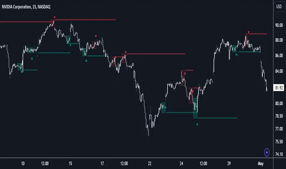
N Bar Reversal Detector [LuxAlgo]The N Bar Reversal Detector is designed to detect and highlight N-bar reversal patterns in user charts, where N represents the length of the candle sequence used to detect the patterns. The script incorporates various trend indicators to filter out detected signals and offers a range of customizable settings to fit different trading strategies.
🔶 USAGE
The N-bar reversal pattern extends the popular 3-bar reversal pattern. While the 3-bar reversal pattern involves identifying a sequence of three bars signaling a potential trend reversal, the N-bar reversal pattern builds on this concept by incorporating additional bars based on user settings. This provides a more comprehensive indication of potential trend reversals. The script automates the identification of these patterns and generates clear, visually distinct signals to highlight potential trend changes.
When a reversal chart pattern is confirmed and aligns with the price action, the pattern's boundaries are extended to create levels. The upper boundary serves as resistance, while the lower boundary acts as support.
The script allows users to filter patterns based on the trend direction identified by various trend indicators. Users can choose to view patterns that align with the detected trend or those that are contrary to it.
🔶 DETAILS
🔹 The N-bar Reversal Pattern
The N-bar reversal pattern is a technical analysis tool designed to signal potential trend reversals in the market. It consists of N consecutive bars, with the first N-1 bars used to identify the prevailing trend and the Nth bar confirming the reversal. Here’s a detailed look at the pattern:
Bullish Reversal : In a bullish reversal setup, the first bar is the highest among the first N-1 bars, indicating a prevailing downtrend. Most of the remaining bars in this sequence should be bearish (closing lower than where they opened), reinforcing the existing downward momentum. The Nth (most recent) bar confirms a bullish reversal if its high price is higher than the high of the first bar in the sequence (standard pattern). For a stronger signal, the closing price of the Nth bar should also be higher than the high of the first bar.
Bearish Reversal : In a bearish reversal setup, the first bar is the lowest among the first N-1 bars, indicating a prevailing uptrend. Most of the remaining bars in this sequence should be bullish (closing higher than where they opened), reinforcing the existing upward momentum. The Nth bar confirms a bearish reversal if its low price is lower than the low of the first bar in the sequence (standard pattern). For a stronger signal, the closing price of the Nth bar should also be lower than the low of the first bar.
🔹 Min Percentage of Required Candles
This parameter specifies the minimum percentage of candles that must be bullish (for a bearish reversal) or bearish (for a bullish reversal) among the first N-1 candles in a pattern. For higher values of N, it becomes more challenging for all of the first N-1 candles to be consistently bullish or bearish. By setting a percentage value, P, users can adjust the requirement so that only a minimum of P percent of the first N-1 candles need to meet the bullish or bearish condition. This allows for greater flexibility in pattern recognition, accommodating variations in market conditions.
🔶 SETTINGS
Pattern Type: Users can choose the type of the N-bar reversal patterns to detect: Normal, Enhanced, or All. "Normal" detects patterns that do not necessarily surpass the high/low of the first bar. "Enhanced" detects patterns where the last bar surpasses the high/low of the first bar. "All" detects both Normal and Enhanced patterns.
Reversal Pattern Sequence Length: Specifies the number of candles (N) in the sequence used to identify a reversal pattern.
Min Percentage of Required Candles: Sets the minimum percentage of the first N-1 candles that must be bullish (for a bearish reversal) or bearish (for a bullish reversal) to qualify as a valid reversal pattern.
Derived Support and Resistance: Toggles the visibility of the support and resistance levels/zones.
🔹 Trend Filtering
Filtering: Allows users to filter patterns based on the trend indicators: Moving Average Cloud, Supertrend, and Donchian Channels. The "Aligned" option only detects patterns that align with the trend and conversely, the "Opposite" option detects patterns that go against the trend.
🔹 Trend Indicator Settings
Moving Average Cloud: Allows traders to choose the type of moving averages (SMA, EMA, HMA, etc.) and set the lengths for fast and slow moving averages.
Supertrend: Options to set the ATR length and factor for Supertrend.
Donchian Channels: Option to set the length for the channel calculation.
🔶 RELATED SCRIPTS
Reversal-Candlestick-Structure.
Reversal-Signals.
Intramarket Difference Index StrategyHi Traders !!
The IDI Strategy:
In layman’s terms this strategy compares two indicators across markets and exploits their differences.
note: it is best the two markets are correlated as then we know we are trading a short to long term deviation from both markets' general trend with the assumption both markets will trend again sometime in the future thereby exhausting our trading opportunity.
📍 Import Notes:
This Strategy calculates trade position size independently (i.e. risk per trade is controlled in the user inputs tab), this means that the ‘Order size’ input in the ‘Properties’ tab will have no effect on the strategy. Why ? because this allows us to define custom position size algorithms which we can use to improve our risk management and equity growth over time. Here we have the option to have fixed quantity or fixed percentage of equity ATR (Average True Range) based stops in addition to the turtle trading position size algorithm.
‘Pyramiding’ does not work for this strategy’, similar to the order size input togeling this input will have no effect on the strategy as the strategy explicitly defines the maximum order size to be 1.
This strategy is not perfect, and as of writing of this post I have not traded this algo.
Always take your time to backtests and debug the strategy.
🔷 The IDI Strategy:
By default this strategy pulls data from your current TV chart and then compares it to the base market, be default BINANCE:BTCUSD . The strategy pulls SMA and RSI data from either market (we call this the difference data), standardizes the data (solving the different unit problem across markets) such that it is comparable and then differentiates the data, calling the result of this transformation and difference the Intramarket Difference (ID). The formula for the the ID is
ID = market1_diff_data - market2_diff_data (1)
Where
market(i)_diff_data = diff_data / ATR(j)_market(i)^0.5,
where i = {1, 2} and j = the natural numbers excluding 0
Formula (1) interpretation is the following
When ID > 0: this means the current market outperforms the base market
When ID = 0: Markets are at long run equilibrium
When ID < 0: this means the current market underperforms the base market
To form the strategy we define one of two strategy type’s which are Trend and Mean Revesion respectively.
🔸 Trend Case:
Given the ‘‘Strategy Type’’ is equal to TREND we define a threshold for which if the ID crosses over we go long and if the ID crosses under the negative of the threshold we go short.
The motivating idea is that the ID is an indicator of the two symbols being out of sync, and given we know volatility clustering, momentum and mean reversion of anomalies to be a stylised fact of financial data we can construct a trading premise. Let's first talk more about this premise.
For some markets (cryptocurrency markets - synthetic symbols in TV) the stylised fact of momentum is true, this means that higher momentum is followed by higher momentum, and given we know momentum to be a vector quantity (with magnitude and direction) this momentum can be both positive and negative i.e. when the ID crosses above some threshold we make an assumption it will continue in that direction for some time before executing back to its long run equilibrium of 0 which is a reasonable assumption to make if the market are correlated. For example for the BTCUSD - ETHUSD pair, if the ID > +threshold (inputs for MA and RSI based ID thresholds are found under the ‘‘INTRAMARKET DIFFERENCE INDEX’’ group’), ETHUSD outperforms BTCUSD, we assume the momentum to continue so we go long ETHUSD.
In the standard case we would exit the market when the IDI returns to its long run equilibrium of 0 (for the positive case the ID may return to 0 because ETH’s difference data may have decreased or BTC’s difference data may have increased). However in this strategy we will not define this as our exit condition, why ?
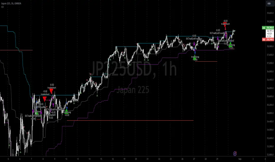
This is because we want to ‘‘let our winners run’’, to achieve this we define a trailing Donchian Channel stop loss (along with a fixed ATR based stop as our volatility proxy). If we were too use the 0 exit the strategy may print a buy signal (ID > +threshold in the simple case, market regimes may be used), return to 0 and then print another buy signal, and this process can loop may times, this high trade frequency means we fail capture the entire market move lowering our profit, furthermore on lower time frames this high trade frequencies mean we pay more transaction costs (due to price slippage, commission and big-ask spread) which means less profit.
By capturing the sum of many momentum moves we are essentially following the trend hence the trend following strategy type.
Here we also print the IDI (with default strategy settings with the MA difference type), we can see that by letting our winners run we may catch many valid momentum moves, that results in a larger final pnl that if we would otherwise exit based on the equilibrium condition(Valid trades are denoted by solid green and red arrows respectively and all other valid trades which occur within the original signal are light green and red small arrows).
another example...
Note: if you would like to plot the IDI separately copy and paste the following code in a new Pine Script indicator template.
indicator("IDI")
// INTRAMARKET INDEX
var string g_idi = "intramarket diffirence index"
ui_index_1 = input.symbol("BINANCE:BTCUSD", title = "Base market", group = g_idi)
// ui_index_2 = input.symbol("BINANCE:ETHUSD", title = "Quote Market", group = g_idi)
type = input.string("MA", title = "Differrencing Series", options = , group = g_idi)
ui_ma_lkb = input.int(24, title = "lookback of ma and volatility scaling constant", group = g_idi)
ui_rsi_lkb = input.int(14, title = "Lookback of RSI", group = g_idi)
ui_atr_lkb = input.int(300, title = "ATR lookback - Normalising value", group = g_idi)
ui_ma_threshold = input.float(5, title = "Threshold of Upward/Downward Trend (MA)", group = g_idi)
ui_rsi_threshold = input.float(20, title = "Threshold of Upward/Downward Trend (RSI)", group = g_idi)
//>>+----------------------------------------------------------------+}
// CUSTOM FUNCTIONS |
//<<+----------------------------------------------------------------+{
// construct UDT (User defined type) containing the IDI (Intramarket Difference Index) source values
// UDT will hold many variables / functions grouped under the UDT
type functions
float Close // close price
float ma // ma of symbol
float rsi // rsi of the asset
float atr // atr of the asset
// the security data
getUDTdata(symbol, malookback, rsilookback, atrlookback) =>
indexHighTF = barstate.isrealtime ? 1 : 0
= request.security(symbol, timeframe = timeframe.period,
expression = [close , // Instentiate UDT variables
ta.sma(close, malookback) ,
ta.rsi(close, rsilookback) ,
ta.atr(atrlookback) ])
data = functions.new(close_, ma_, rsi_, atr_)
data
// Intramerket Difference Index
idi(type, symbol1, malookback, rsilookback, atrlookback, mathreshold, rsithreshold) =>
threshold = float(na)
index1 = getUDTdata(symbol1, malookback, rsilookback, atrlookback)
index2 = getUDTdata(syminfo.tickerid, malookback, rsilookback, atrlookback)
// declare difference variables for both base and quote symbols, conditional on which difference type is selected
var diffindex1 = 0.0, var diffindex2 = 0.0,
// declare Intramarket Difference Index based on series type, note
// if > 0, index 2 outpreforms index 1, buy index 2 (momentum based) until equalibrium
// if < 0, index 2 underpreforms index 1, sell index 1 (momentum based) until equalibrium
// for idi to be valid both series must be stationary and normalised so both series hae he same scale
intramarket_difference = 0.0
if type == "MA"
threshold := mathreshold
diffindex1 := (index1.Close - index1.ma) / math.pow(index1.atr*malookback, 0.5)
diffindex2 := (index2.Close - index2.ma) / math.pow(index2.atr*malookback, 0.5)
intramarket_difference := diffindex2 - diffindex1
else if type == "RSI"
threshold := rsilookback
diffindex1 := index1.rsi
diffindex2 := index2.rsi
intramarket_difference := diffindex2 - diffindex1
//>>+----------------------------------------------------------------+}
// STRATEGY FUNCTIONS CALLS |
//<<+----------------------------------------------------------------+{
// plot the intramarket difference
= idi(type,
ui_index_1,
ui_ma_lkb,
ui_rsi_lkb,
ui_atr_lkb,
ui_ma_threshold,
ui_rsi_threshold)
//>>+----------------------------------------------------------------+}
plot(intramarket_difference, color = color.orange)
hline(type == "MA" ? ui_ma_threshold : ui_rsi_threshold, color = color.green)
hline(type == "MA" ? -ui_ma_threshold : -ui_rsi_threshold, color = color.red)
hline(0)
Note it is possible that after printing a buy the strategy then prints many sell signals before returning to a buy, which again has the same implication (less profit. Potentially because we exit early only for price to continue upwards hence missing the larger "trend"). The image below showcases this cenario and again, by allowing our winner to run we may capture more profit (theoretically).
This should be clear...
🔸 Mean Reversion Case:
We stated prior that mean reversion of anomalies is an standerdies fact of financial data, how can we exploit this ?
We exploit this by normalizing the ID by applying the Ehlers fisher transformation. The transformed data is then assumed to be approximately normally distributed. To form the strategy we employ the same logic as for the z score, if the FT normalized ID > 2.5 (< -2.5) we buy (short). Our exit conditions remain unchanged (fixed ATR stop and trailing Donchian Trailing stop)
🔷 Position Sizing:
If ‘‘Fixed Risk From Initial Balance’’ is toggled true this means we risk a fixed percentage of our initial balance, if false we risk a fixed percentage of our equity (current balance).
Note we also employ a volatility adjusted position sizing formula, the turtle training method which is defined as follows.
Turtle position size = (1/ r * ATR * DV) * C
Where,
r = risk factor coefficient (default is 20)
ATR(j) = risk proxy, over j times steps
DV = Dollar Volatility, where DV = (1/Asset Price) * Capital at Risk
🔷 Risk Management:
Correct money management means we can limit risk and increase reward (theoretically). Here we employ
Max loss and gain per day
Max loss per trade
Max number of consecutive losing trades until trade skip
To read more see the tooltips (info circle).
🔷 Take Profit:
By defualt the script uses a Donchain Channel as a trailing stop and take profit, In addition to this the script defines a fixed ATR stop losses (by defualt, this covers cases where the DC range may be to wide making a fixed ATR stop usefull), ATR take profits however are defined but optional.
ATR SL and TP defined for all trades
🔷 Hurst Regime (Regime Filter):
The Hurst Exponent (H) aims to segment the market into three different states, Trending (H > 0.5), Random Geometric Brownian Motion (H = 0.5) and Mean Reverting / Contrarian (H < 0.5). In my interpretation this can be used as a trend filter that eliminates market noise.
We utilize the trending and mean reverting based states, as extra conditions required for valid trades for both strategy types respectively, in the process increasing our trade entry quality.
🔷 Example model Architecture:
Here is an example of one configuration of this strategy, combining all aspects discussed in this post.
Future Updates
- Automation integration (next update)
VIX Bars [CrossTrade]In simple terms, this indicator colors your chart bars based on the VIX levels. We know that high volatility is unstainable and will naturally regress to a calmer market, therefore highlighting the bars where VIX is at extreme highs can sometimes indicate a market turning point. Consider pairing this indicator with my VIX Heatmap indicator for a complete picture of volatility.
Customizable VIX Levels: You can set your own thresholds for when the bars turn green or red. Green bars pop up when the VIX is above your set upper level (default is 30) - kind of like a heads-up that things might get bumpy. Red bars show up when the VIX dips below your lower threshold (default is 15), signaling calmer waters.
Optional Donchian Channel Filter: The Donchian Channel filter looks at the highest highs and lowest lows over your chosen period (default's 52 days) and only colors the bars if they match the filter's criteria. This adds an extra layer of confirmation that the colored bars at at a major high or low.
Visual Simplicity: The indicator keeps things visually straightforward. No cluttered screen, just colored bars telling you a story about market vibes. Alert come standard to signal those potential bottom or top bars based on the VIX being at your preferred extreme levels.
In essence, "VIX Bars" is like having a volatility radar on your chart. It doesn't make predictions, but it sure gives you a neat, color-coded heads-up on market sentiment. Great for adding an extra dimension to your analysis without getting all tangled up in complex indicators!

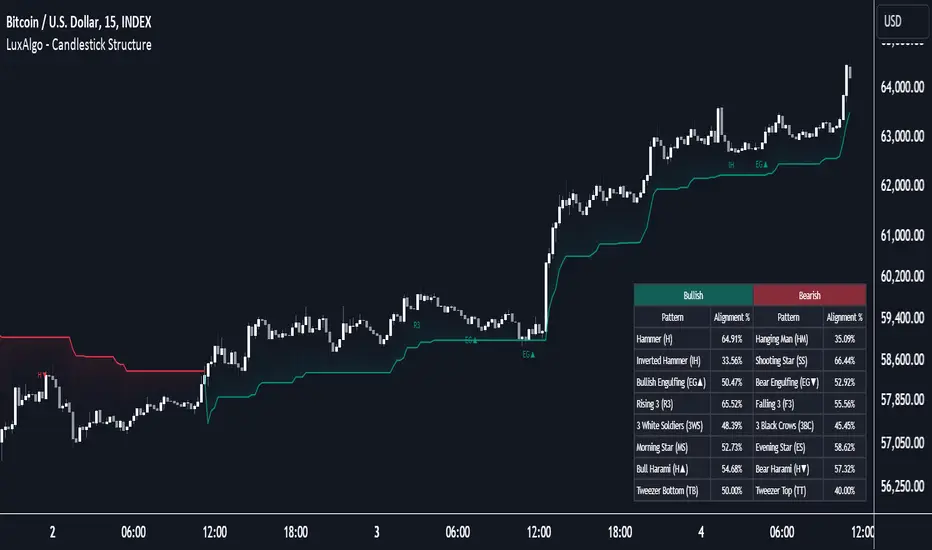
Candlestick Structure [LuxAlgo]The Candlestick Structure indicator detects major market trends and displays various candlestick patterns aligning with the detected trend, filtering out potentially unwanted patterns as a result. Multiple trend detection methods are included and can be selected by the users.
A dashboard showing the alignment percentage of each individual pattern is also provided.
🔶 USAGE
By distinguishing major and minor trend detection, we can still detect patterns based on minor trends, yet filter out the patterns that do not align with the major trend.
By detecting candlestick patterns that align with a major trend, we can effectively detect the ending points of retracements, potentially providing various entry points of interest within a trend.
Users are able to track the alignment of each candlestick pattern in the dashboard to reveal which patterns typically align with the trend and which may not.
Note: Alignment % only checks if the pattern's direction is the same as the current trend direction. These are only raw readings and not any type of confidence score.
🔶 DETAILS
In this indicator, we are identifying and tracking 16 different Candlestick Patterns.
🔹 Bullish Patterns
Hammer: Identified by a small upper wick (or no upper wick) with a small body, and an elongated lower wick whose length is 2X greater than the candle body’s width.
Inverted Hammer: Identified by a small lower wick (or no lower wick) with a small body, and an elongated upper wick whose length is 2X greater than the candle body’s width.
Bullish Engulfing: A 2 bar pattern identified by a large bullish candle body fully encapsulating (opening lower and closing higher) the previous small (bearish) candle body.
Rising 3: A 5 bar pattern identified by an initial full-bodied bullish candle, followed by 3 bearish candles that trade within the high and low of the initial candle, followed by another full-bodied bullish candle closing above the high of the initial candle.
3 White Soldiers: Identified by 3 full-bodied bullish candles, each opening within the body and closing below the high, of the previous candle.
Morning Star: A 3 bar pattern identified by a full-bodied bearish candle, followed by a small-bodied bearish candle, followed by a full-bodied bullish candle that closes above the halfway point of the first candle.
Bullish Harami: A 2 bar pattern, identified by an initial bearish candle, followed by a small bullish candle whose range is entirely contained within the body of the initial candle.
Tweezer Bottom: A 2 bar pattern identified by an initial bearish candle, followed by a bullish candle, both having equal lows.
🔹 Bearish Patterns
Hanging Man: Identified by a small upper wick (or no upper wick) with a small body, and an elongated lower wick whose length is 2X greater than the candle body’s width.
Shooting Star: Identified by a small lower wick (or no lower wick) with a small body, and an elongated upper wick whose length is 2X greater than the candle body’s width.
Bearish Engulfing: A 2 bar pattern identified by a large bearish candle body fully encapsulating (opening higher and closing lower) the previous small (bullish) candle body.
Falling 3: A 5 bar pattern identified by an initial full-bodied bearish candle, followed by 3 bullish candles that trade within the high and low of the initial candle, followed by another full-bodied bearish candle closing below the low of the initial candle.
3 Black Crows: Identified by 3 full-bodied bearish candles, each open within the body and closing below the low, of the previous candle.
Evening Star: A 3 bar pattern identified by a full-bodied bullish candle, followed by a small-bodied bullish candle, followed by a full-bodied bearish candle that closes below the halfway point of the first candle.
Bearish Harami: A 2 bar pattern, identified by an initial bullish candle, followed by a small bearish candle whose range is entirely contained within the body of the initial candle.
Tweezer Top: A 2 bar pattern identified by an initial bullish candle, followed by a bearish candle, both having equal highs.
🔹 Trend Types
Major trend is displayed at all times, the display will change depending on the trend method selected.
The minor trend can also be visualized; to avoid confusion, the minor trend can optionally be displayed through the candle colors.
Supertrend: Displays Upper and Lower SuperTrend, When we break above the upper, it is considered an Uptrend. When we break below the lower, it is considered a Downtrend.
EMAs: Displays Fast and Slow EMAs, When Fast>Slow, it is considered an Uptrend. When Fast
DeQuex Algo BISTIntroduction:
The DeQuex Algo is an advanced technical analysis tool designed to help traders identify high-probability entry and exit points in the Borsa Istanbul (BIST) market. This updated version incorporates an adaptive MACD to reduce false signals and improve the overall reliability of the indicator.
Key Features:
1. Adaptive MACD: The script utilizes an adaptive MACD that dynamically adjusts to market volatility, reducing the occurrence of false signals often associated with traditional MACD implementations.
2. RSI Confirmation: In addition to the adaptive MACD, the DeQuex Algo also considers RSI readings to provide stronger confirmation for buy and sell signals.
3. Signal Types:
- Buy Signal: Triggered when the adaptive MACD crosses above its signal line.
- Sell Signal: Triggered when the adaptive MACD crosses below its signal line.
- Strong Buy Signal: Triggered when both the adaptive MACD and RSI cross above their respective thresholds, indicating a high-probability bullish setup.
- Strong Sell Signal: Triggered when both the adaptive MACD and RSI cross below their respective thresholds, indicating a high-probability bearish setup.
4. Price Bar Highlighting: The script color-codes price bars to provide a visual representation of the current trend. Green bars indicate an uptrend, red bars indicate a downtrend, and purple bars signify a period of consolidation or uncertainty. This feature allows traders to quickly assess the market context at a glance.
5. Customizable Alerts: Users can enable alerts for each signal type, ensuring they never miss a potential trading opportunity.
6. Dynamic Support and Resistance: The DeQuex Algo incorporates dynamic support and resistance levels based on market volatility. These levels are plotted using an innovative approach that combines Donchian channels with a Kalman filter for smoother, more reliable zones.
7. User-Friendly Inputs: The script provides a range of input parameters, allowing traders to fine-tune the indicator's sensitivity and adapt it to their preferred trading style and timeframe.
How to Use:
1. Add the DeQuex Algo indicator to your TradingView chart.
2. Customize the input parameters as desired, or use the default settings.
3. Enable alerts for your preferred signal types.
4. Look for buy and sell signals based on the adaptive MACD and RSI readings, paying attention to the color-coded price bars for additional context.
5. Consider the dynamic support and resistance levels when planning your entries, exits, and stop-loss placements.
Please note that while the DeQuex Algo is designed to identify high-probability setups, no indicator is perfect, and false signals may still occur. Always use proper risk management and consider other factors, such as market sentiment and fundamental analysis, when making trading decisions.
We hope that the DeQuex Algo will be a valuable addition to your trading toolbox, and we welcome any feedback or suggestions for further improvement.
Best regards,
BrandonJames1337
TR:
İşte güncellenmiş DeQuex Algo göstergeniz için önerilen bir açıklama:
Giriş:
DeQuex Algo, yatırımcıların Borsa İstanbul (BIST) piyasasında yüksek olasılıklı giriş ve çıkış noktalarını belirlemelerine yardımcı olmak için tasarlanmış gelişmiş bir teknik analiz aracıdır. Bu güncellenmiş sürüm, yanlış sinyalleri azaltmak ve göstergenin genel güvenilirliğini artırmak için uyarlanabilir bir MACD içerir.
Temel Özellikler:
1. Uyarlanabilir MACD: Komut dosyası, piyasa oynaklığına dinamik olarak ayarlanan ve genellikle geleneksel MACD uygulamalarıyla ilişkili yanlış sinyallerin oluşumunu azaltan uyarlanabilir bir MACD kullanır.
2. RSI Onayı: Uyarlanabilir MACD'ye ek olarak DeQuex Algo, alım ve satım sinyalleri için daha güçlü onay sağlamak üzere RSI okumalarını da dikkate alır.
3. Sinyal Türleri:
- Alış Sinyali: Uyarlanabilir MACD sinyal çizgisinin üzerine çıktığında tetiklenir.
- Satış Sinyali: Uyarlanabilir MACD sinyal çizgisinin altından geçtiğinde tetiklenir.
- Güçlü Alış Sinyali: Hem uyarlanabilir MACD hem de RSI kendi eşiklerinin üzerine çıktığında tetiklenir ve yüksek olasılıklı bir yükseliş düzenine işaret eder.
- Güçlü Satış Sinyali: Hem uyarlanabilir MACD hem de RSI kendi eşiklerinin altına düştüğünde tetiklenir ve yüksek olasılıklı bir düşüş düzenine işaret eder.
4. Fiyat Çubuğu Vurgulama: Komut dosyası, mevcut eğilimin görsel bir temsilini sağlamak için fiyat çubuklarını renk kodlarıyla kodlar. Yeşil çubuklar yükseliş trendini, kırmızı çubuklar düşüş trendini ve mor çubuklar ise konsolidasyon veya belirsizlik dönemini gösterir. Bu özellik, yatırımcıların piyasa bağlamını bir bakışta hızlı bir şekilde değerlendirmelerine olanak tanır.
5. Özelleştirilebilir Uyarılar: Kullanıcılar her sinyal türü için uyarıları etkinleştirerek potansiyel bir alım satım fırsatını asla kaçırmamalarını sağlayabilir.
6. Dinamik Destek ve Direnç: DeQuex Algo, piyasa oynaklığına dayalı dinamik destek ve direnç seviyeleri içerir. Bu seviyeler, daha yumuşak ve daha güvenilir bölgeler için Donchian kanallarını Kalman filtresiyle birleştiren yenilikçi bir yaklaşım kullanılarak çizilir.
7. Kullanıcı Dostu Girişler: Komut dosyası, yatırımcıların göstergenin hassasiyetini ince ayarlamalarına ve tercih ettikleri ticaret tarzına ve zaman dilimine uyarlamalarına olanak tanıyan bir dizi giriş parametresi sağlar.
Nasıl Kullanılır:
1. DeQuex Algo göstergesini TradingView grafiğinize ekleyin.
2. Giriş parametrelerini istediğiniz gibi özelleştirin veya varsayılan ayarları kullanın.
3. Tercih ettiğiniz sinyal türleri için uyarıları etkinleştirin.
4. Ek bağlam için renk kodlu fiyat çubuklarına dikkat ederek uyarlanabilir MACD ve RSI okumalarına dayalı alım ve satım sinyallerini arayın.
5. Girişlerinizi, çıkışlarınızı ve stop-loss yerleşimlerinizi planlarken dinamik destek ve direnç seviyelerini göz önünde bulundurun.
DeQuex Algo yüksek olasılıklı kurulumları belirlemek için tasarlanmış olsa da, hiçbir göstergenin mükemmel olmadığını ve yine de yanlış sinyallerin oluşabileceğini lütfen unutmayın. Alım satım kararları verirken her zaman uygun risk yönetimini kullanın ve piyasa duyarlılığı ve temel analiz gibi diğer faktörleri göz önünde bulundurun.
DeQuex Algo'nun ticaret araç kutunuza değerli bir katkı sağlayacağını umuyor ve daha fazla iyileştirme için her türlü geri bildirim veya öneriyi memnuniyetle karşılıyoruz.
Saygılarımla,
BrandonJames1337

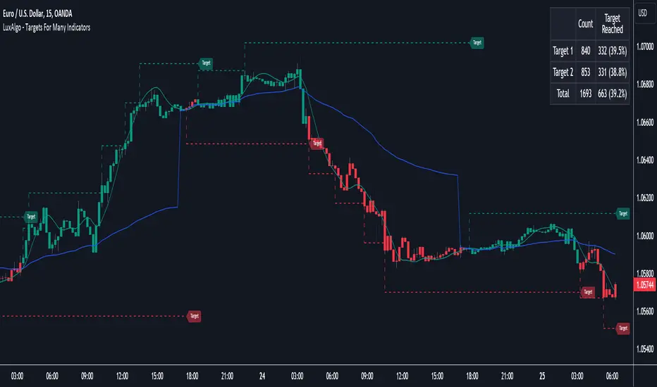
Targets For Many Indicators [LuxAlgo]The Targets For Many Indicators is a useful utility tool able to display targets for many built-in indicators as well as external indicators. Targets can be set for specific user-set conditions between two series of values, with the script being able to display targets for two different user-set conditions.
Alerts are included for the occurrence of a new target as well as for reached targets.
🔶 USAGE
Targets can help users determine the price limit where the price might start deviating from an indication given by one or multiple indicators. In the context of trading, targets can help secure profits/reduce losses of a trade, as such this tool can be useful to evaluate/determine user take profits/stop losses.
Due to these essentially being horizontal levels, they can also serve as potential support/resistances, with breakouts potentially confirming new trends.
In the above example, we set targets 3 ATR's away from the closing price when the price crosses over the script built-in SuperTrend indicator using ATR period 10 and factor 3. Using "Long Position Target" allows setting a target above the price, disabling this setting will place targets below the price.
Users might be interested in obtaining new targets once one is reached, this can be done by enabling "New Target When Reached" in the target logic setting section, resulting in more frequent targets.
Lastly, users can restrict new target creation until current ones are reached. This can result in fewer and longer-term targets, with a higher reach rate.
🔹 Dashboard
A dashboard is displayed on the top right of the chart, displaying the amount, reach rate of targets 1/2, and total amount.
This dashboard can be useful to evaluate the selected target distances relative to the selected conditions, with a higher reach rate suggesting the distance of the targets from the price allows them to be reached.
🔶 DETAILS
🔹 Indicators
Besides 'External' sources, each source can be set at 1 of the following Build-In Indicators :
ACCDIST : Accumulation/distribution index
ATR : Average True Range
BB (Middle, Upper or Lower): Bollinger Bands
CCI : Commodity Channel Index
CMO : Chande Momentum Oscillator
COG : Center Of Gravity
DC (High, Mid or Low): Donchian Channels
DEMA : Double Exponential Moving Average
EMA : Exponentially weighted Moving Average
HMA : Hull Moving Average
III : Intraday Intensity Index
KC (Middle, Upper or Lower): Keltner Channels
LINREG : Linear regression curve
MACD (macd, signal or histogram): Moving Average Convergence/Divergence
MEDIAN : median of the series
MFI : Money Flow Index
MODE : the mode of the series
MOM : Momentum
NVI : Negative Volume Index
OBV : On Balance Volume
PVI : Positive Volume Index
PVT : Price-Volume Trend
RMA : Relative Moving Average
ROC : Rate Of Change
RSI : Relative Strength Index
SMA : Simple Moving Average
STOCH : Stochastic
Supertrend
TEMA : Triple EMA or Triple Exponential Moving Average
VWAP : Volume Weighted Average Price
VWMA : Volume-Weighted Moving Average
WAD : Williams Accumulation/Distribution
WMA : Weighted Moving Average
WVAD : Williams Variable Accumulation/Distribution
%R : Williams %R
Each indicator is provided with a link to the Reference Manual or to the Build-In Indicators page.
The latter contains more information about each indicator.
Note that when "Show Source Values" is enabled, only values that can be logically found around the price will be shown. For example, Supertrend , SMA , EMA , BB , ... will be made visible. Values like RSI , OBV , %R , ... will not be visible since they will deviate too much from the price.
🔹 Interaction with settings
This publication contains input fields, where you can enter the necessary inputs per indicator.
Some indicators need only 1 value, others 2 or 3.
When several input values are needed, you need to separate them with a comma.
You can use 0 to 4 spaces between without a problem. Even an extra comma doesn't give issues.
The red colored help text will guide you further along (Only when Target is enabled)
Some examples that work without issues:
Some examples that work with issues:
As mentioned, the errors won't be visible when the concerning target is disabled
🔶 SETTINGS
Show Target Labels: Display target labels on the chart.
Candle Coloring: Apply candle coloring based on the most recent active target.
Target 1 and Target 2 use the same settings below:
Enable Target: Display the targets on the chart.
Long Position Target: Display targets above the price a user selected condition is true. If disabled will display the targets below the price.
New Target Condition: Conditional operator used to compare "Source A" and "Source B", options include CrossOver, CrossUnder, Cross, and Equal.
🔹 Sources
Source A: Source A input series, can be an indicator or external source.
External: External source if 'External" is selected in "Source A".
Settings: Settings of the selected indicator in "Source A", entered settings of indicators requiring multiple ones must be comma separated, for example, "10, 3".
Source B: Source B input series, can be an indicator or external source.
External: External source if 'External" is selected in "Source B".
Settings: Settings of the selected indicator in "Source B", entered settings of indicators requiring multiple ones must be comma separated, for example, "10, 3".
Source B Value: User-defined numerical value if "value" is selected in "Source B".
Show Source Values: Display "Source A" and "Source B" on the chart.
🔹 Logic
Wait Until Reached: When enabled will not create a new target until an existing one is reached.
New Target When Reached: Will create a new target when an existing one is reached.
Evaluate Wicks: Will use high/low prices to determine if a target is reached. Unselecting this setting will use the closing price.
Target Distance From Price: Controls the distance of a target from the price. Can be determined in currencies/points, percentages, ATR multiples, ticks, or using multiple of external values.
External Distance Value: External distance value when "External Value" is selected in "Target Distance From Price".
hamster-bot MRS 2 (simplified version) MRS - Mean Reversion Strategy (Countertrend) (Envelope strategy)
This script does not claim to be unique and does not mislead anyone. Even the unattractive backtest result is attached. The source code is open. The idea has been described many times in various sources. But at the same time, their collection in one place provides unique opportunities.
Published by popular demand and for ease of use. so that users can track the development of the script and can offer their ideas in the comments. Otherwise, you have to communicate in several telegram chats.
Representative of the family of counter-trend strategies. The basis of the strategy is Mean reversion . You can also read about the Envelope strategy .
Mean reversion , or reversion to the mean, is a theory used in finance that suggests that asset price volatility and historical returns eventually will revert to the long-run mean or average level of the entire dataset.
The strategy is very simple. Has very few settings. Good for beginners to get acquainted with algorithmic trading. A simple adjustment will help avoid overfitting. There are many variations of this strategy, but for understanding it is better to start with this implementation.
Principle of operation.
1)
A conventional MA is being built. (fuchsia line). A limit order is placed on this line to close the position.
2)
(green line) A limit order is placed on this line to open a long position
3)
(red line) A limit order is placed on this line to open a short position
Attention!
Please note that a limit order is used. Conclude that the strategy has a limited capacity. And the results obtained on low-liquid instruments will be too high in the tester. On real auctions there will be a different result.
Note for testing the strategy in the spot market:
When testing in the spot market, do not include both long and short at the same time. It is recommended to test only the long mode on the spot. Short mode for more advanced users.
Settings:
Available types of moving averages:
SMA
EMA
TEMA - triple exponential moving average
DEMA - Double Exponential Moving Average
ZLEMA - Zero lag exponential moving average
WMA - weighted moving average
Hma - Hull Moving Average
Thma - Triple Exponential Hull Moving Average
Ehma - Exponential Hull Moving Average
H - MA built based on highs for n candles | ta.highest(len)
L - MA built based on lows for n candles | ta.lowest(len)
DMA - Donchian Moving Average
A Kalman filter can be applied to all MA
The peculiarity of the strategy is a large selection of MA and the possibility of shifting lines. You can set up a reverse trending strategy on the Donchian channel for example.
Use Long - enable/disable opening a Long position
Use Short - enable/disable opening a Short position
Lot Long, % - % allocated from the deposit for opening a Long position. In the spot market, do not use % greater than 100%
Lot Short, % - allocated % of the deposit for opening a Short position
Start date - the beginning of the testing period
End date - the end of the testing period (Example: only August 2020 can be tested)
Mul - multiplier. Used to offset lines. Example:
Mul = 0.99 is shift -1%
Mul = 1.01 is shift +1%
Non-strict recommendations:
1) Test the SPOT market on crypto exchanges. (The countertrend strategy has liquidation risk on futures)
2) Symbols altcoin/bitcoin or altcoin/altcoin. Example: ETH/BTC or DOGE/ETH
3) Timeframe is usually 1 hour
If the script passes moderation, I will supplement it by adding separate settings for closing long and short positions according to their MA

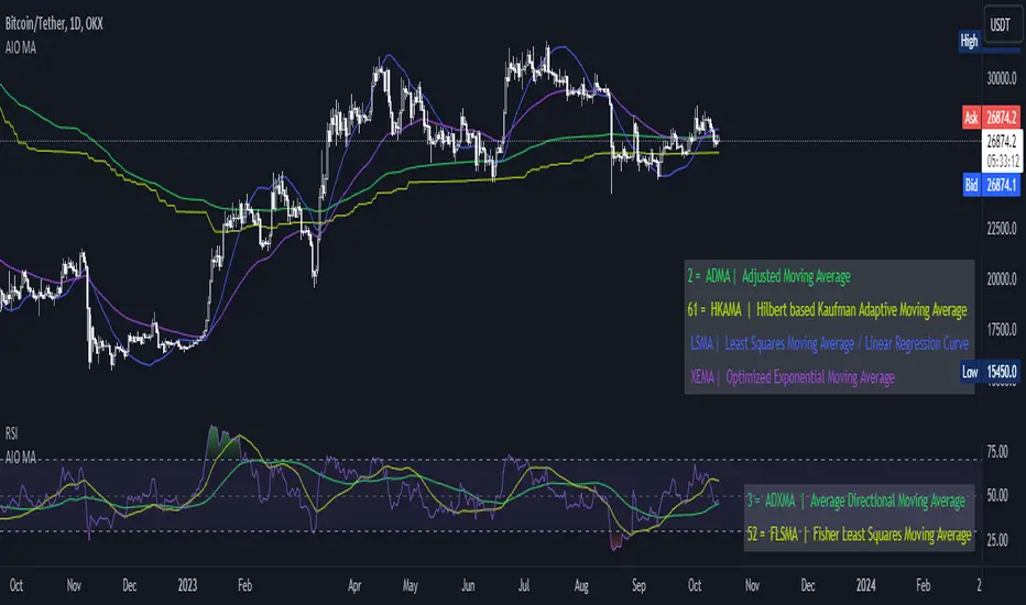
[AIO] Multi Collection Moving Averages 140 MA TypesAll In One Multi Collection Moving Averages.
Since signing up 2 years ago, I have been collecting various Сollections.
I decided to get it into a decent shape and make it one of the biggest collections on TV, and maybe the entire internet.
And now I'm sharing my collection with you.
140 Different Types of Moving Averages are waiting for you.
Specifically :
"
AARMA | Adaptive Autonomous Recursive Moving Average
ADMA | Adjusted Moving Average
ADXMA | Average Directional Moving Average
ADXVMA | Average Directional Volatility Moving Average
AHMA | Ahrens Moving Average
ALF | Ehler Adaptive Laguerre Filter
ALMA | Arnaud Legoux Moving Average
ALSMA | Adaptive Least Squares
ALXMA | Alexander Moving Average
AMA | Adaptive Moving Average
ARI | Unknown
ARSI | Adaptive RSI Moving Average
AUF | Auto Filter
AUTL | Auto-Line
BAMA | Bryant Adaptive Moving Average
BFMA | Blackman Filter Moving Average
CMA | Corrected Moving Average
CORMA | Correlation Moving Average
COVEMA | Coefficient of Variation Weighted Exponential Moving Average
COVNA | Coefficient of Variation Weighted Moving Average
CTI | Coral Trend Indicator
DEC | Ehlers Simple Decycler
DEMA | Double EMA Moving Average
DEVS | Ehlers - Deviation Scaled Moving Average
DONEMA | Donchian Extremum Moving Average
DONMA | Donchian Moving Average
DSEMA | Double Smoothed Exponential Moving Average
DSWF | Damped Sine Wave Weighted Filter
DWMA | Double Weighted Moving Average
E2PBF | Ehlers 2-Pole Butterworth Filter
E2SSF | Ehlers 2-Pole Super Smoother Filter
E3PBF | Ehlers 3-Pole Butterworth Filter
E3SSF | Ehlers 3-Pole Super Smoother Filter
EDMA | Exponentially Deviating Moving Average (MZ EDMA)
EDSMA | Ehlers Dynamic Smoothed Moving Average
EEO | Ehlers Modified Elliptic Filter Optimum
EFRAMA | Ehlers Modified Fractal Adaptive Moving Average
EHMA | Exponential Hull Moving Average
EIT | Ehlers Instantaneous Trendline
ELF | Ehler Laguerre filter
EMA | Exponential Moving Average
EMARSI | EMARSI
EPF | Edge Preserving Filter
EPMA | End Point Moving Average
EREA | Ehlers Reverse Exponential Moving Average
ESSF | Ehlers Super Smoother Filter 2-pole
ETMA | Exponential Triangular Moving Average
EVMA | Elastic Volume Weighted Moving Average
FAMA | Following Adaptive Moving Average
FEMA | Fast Exponential Moving Average
FIBWMA | Fibonacci Weighted Moving Average
FLSMA | Fisher Least Squares Moving Average
FRAMA | Ehlers - Fractal Adaptive Moving Average
FX | Fibonacci X Level
GAUS | Ehlers - Gaussian Filter
GHL | Gann High Low
GMA | Gaussian Moving Average
GMMA | Geometric Mean Moving Average
HCF | Hybrid Convolution Filter
HEMA | Holt Exponential Moving Average
HKAMA | Hilbert based Kaufman Adaptive Moving Average
HMA | Harmonic Moving Average
HSMA | Hirashima Sugita Moving Average
HULL | Hull Moving Average
HULLT | Hull Triple Moving Average
HWMA | Henderson Weighted Moving Average
IE2 | Early T3 by Tim Tilson
IIRF | Infinite Impulse Response Filter
ILRS | Integral of Linear Regression Slope
JMA | Jurik Moving Average
KA | Unknown
KAMA | Kaufman Adaptive Moving Average & Apirine Adaptive MA
KIJUN | KIJUN
KIJUN2 | Kijun v2
LAG | Ehlers - Laguerre Filter
LCLSMA | 1LC-LSMA (1 line code lsma with 3 functions)
LEMA | Leader Exponential Moving Average
LLMA | Low-Lag Moving Average
LMA | Leo Moving Average
LP | Unknown
LRL | Linear Regression Line
LSMA | Least Squares Moving Average / Linear Regression Curve
LTB | Unknown
LWMA | Linear Weighted Moving Average
MAMA | MAMA - MESA Adaptive Moving Average
MAVW | Mavilim Weighted Moving Average
MCGD | McGinley Dynamic Moving Average
MF | Modular Filter
MID | Median Moving Average / Percentile Nearest Rank
MNMA | McNicholl Moving Average
MTMA | Unknown
MVSMA | Minimum Variance SMA
NLMA | Non-lag Moving Average
NWMA | Dürschner 3rd Generation Moving Average (New WMA)
PKF | Parametric Kalman Filter
PWMA | Parabolic Weighted Moving Average
QEMA | Quadruple Exponential Moving Average
QMA | Quick Moving Average
REMA | Regularized Exponential Moving Average
REPMA | Repulsion Moving Average
RGEMA | Range Exponential Moving Average
RMA | Welles Wilders Smoothing Moving Average
RMF | Recursive Median Filter
RMTA | Recursive Moving Trend Average
RSMA | Relative Strength Moving Average - based on RSI
RSRMA | Right Sided Ricker MA
RWMA | Regressively Weighted Moving Average
SAMA | Slope Adaptive Moving Average
SFMA | Smoother Filter Moving Average
SMA | Simple Moving Average
SSB | Senkou Span B
SSF | Ehlers - Super Smoother Filter P2
SSMA | Super Smooth Moving Average
STMA | Unknown
SWMA | Self-Weighted Moving Average
SW_MA | Sine-Weighted Moving Average
TEMA | Triple Exponential Moving Average
THMA | Triple Exponential Hull Moving Average
TL | Unknown
TMA | Triangular Moving Average
TPBF | Three-pole Ehlers Butterworth
TRAMA | Trend Regularity Adaptive Moving Average
TSF | True Strength Force
TT3 | Tilson (3rd Degree) Moving Average
VAMA | Volatility Adjusted Moving Average
VAMAF | Volume Adjusted Moving Average Function
VAR | Vector Autoregression Moving Average
VBMA | Variable Moving Average
VHMA | Vertical Horizontal Moving Average
VIDYA | Variable Index Dynamic Average
VMA | Volume Moving Average
VSO | Unknown
VWMA | Volume Weighted Moving Average
WCD | Unknown
WMA | Weighted Moving Average
XEMA | Optimized Exponential Moving Average
ZEMA | Zero Lag Moving Average
ZLDEMA | Zero-Lag Double Exponential Moving Average
ZLEMA | Ehlers - Zero Lag Exponential Moving Average
ZLTEMA | Zero-Lag Triple Exponential Moving Average
ZSMA | Zero-Lag Simple Moving Average
"
Don't forget that you can use any Moving Average not only for the chart but also for any of your indicators without affecting the code as in my example.
But remember that some MAs are not designed to work with anything other than a chart.
All MA and Code lists are sorted strictly alphabetically by short name (A-Z).
Each MA has its own number (ID) by which you can display the Moving Average you need.
Next to the ID selection there are tooltips with short names and their numbers. Use them.
The panel below will help you to read the Name of the selected MA.
Because of the size of the collection I think this is the optimal and most convenient use. Correct me if this is not the case.
Unknown - Some MAs I collected so long ago that I lost the full real name and couldn't find the authors. If you recognize them, please let me know.
I have deliberately simplified all MAs to input just Source and Length.
Because the collection is so large, it would be quite inconvenient and difficult to customize all MA functions (multipliers, offset, etc.).
If you need or like any MA you will still have to take it from my collection for your code.
I tried to leave the basic MA settings inside function in first strings.
I have tried to list most of the authors, but since the bulk of the collection was created a long time ago and was not intended for public publication I could not find all of them.
Some of the features were created from scratch or may have been slightly modified, so please be careful.
If you would like to improve this collection, please write to me in PM.
Also Credits, Likes, Awards, Loves and Thanks to :
@alexgrover
@allanster
@andre_007
@auroagwei
@blackcat1402
@bsharpe
@cheatcountry
@CrackingCryptocurrency
@Duyck
@ErwinBeckers
@everget
@glaz
@gotbeatz26107
@HPotter
@io72signals
@JacobAmos
@JoshuaMcGowan
@KivancOzbilgic
@LazyBear
@loxx
@LuxAlgo
@MightyZinger
@nemozny
@NGBaltic
@peacefulLizard50262
@RicardoSantos
@StalexBot
@ThiagoSchmitz
@TradingView
— 𝐀𝐧𝐝 𝐎𝐭𝐡𝐞𝐫𝐬 !
So just a Big Thank You to everyone who has ever and anywhere shared their codes.
X48 - Strategy | BreakOut & Consecutive (11in1) + Alert | V.1.2================== Read This First Before Use This Strategy ==============
*********** Please be aware that this strategy is not a guarantee of success and may lead to losses.
*********** Trading involves risk and you should always do your own research before making any decisions.
================= Thanks Source Script and Explain This Strategy ===================
► Description
Write a detailed and meaningful description that allows users to understand how your script is original, what it does, how it does it and how to use it
This Strategy Are Combine Strategy and Indicators Alert Function For Systematic Trading User.
Strategy List, Thanks For Original Source Script , From Tradingview Build-in Script From fmzquant Github
// Channel BreakOut Strategy : Calculate BreakOut Zone For Buy and Sell.
// Consecutive Bars UP/Down Strategy : The consecutive bars up/down strategy is a trading strategy used to identify potential buy and sell signals in the stock market. This strategy involves looking for a series of bars (or candles) that are either all increasing or all decreasing in price. If the bars are all increasing, it can be a signal to buy, and if the bars are all decreasing, it can be a signal to sell. This strategy can be used on any timeframe, from a daily chart to an intraday chart.
// 15m Range Length SD : Range Of High and Low Candle Price and Lookback For Calculate Buy and Sell.
Indicators Are Simple Source Script (Almost I'm Chating With CHAT-GPT and Convert pinescript V4 to V5 again for complete almost script and combine after)
// SwingHigh and SwingLow Plot For SL (StopLoss by Last Swing).
// Engulfing and 3 Candle Engulfing Plot.
// Stochastic RSI for Plot and Fill Background Paint and Plot TEXT For BULL and BEAR TREND.
// MA TYPE MODE are plot 2 line of MA Type (EMA, SMA, HMA, WMA, VWMA) for Crossover and Crossunder.
// Donchian Fans MODE are Plot Dot Line With Triangle Degree Bull Trend is Green Plot and Bear Trend is Red Plot.
// Ichimoku Cloud Are Plot Cloud A-B For Bull and Bear Trend.
// RSI OB and OS for TEXT PLOT 'OB' , 'OS' you will know after OB and OS, you can combo with other indicators that's make you know what's the similar trend look like?
// MACD for Plot Diamond when MACD > 0 and MACD < 0, you can combo with other indicators that's make you know what's the similar trend look like?
Alert Can Alert Sent When Buy and Sell or TP and SL, you can adjust text to alert sent by your self or use default setting.
========== Let'e Me Explain How To Use This Strategy =============
========== Properties Setting ==========
// Capital : Default : 1,000 USDT For Alot Of People Are Beginner Investor = It's Capital Your Cash For Investment
// Ordersize : Default Are Setting 5% / Order We Call Compounded
========== INPUT Setting ==========
// First Part Use Must Choose Checkbox For Use of Strategy and Choose TP/SL by Swing or % (can choose both)
// In Detail Of Setting Are Not Too Much, Please Read The Header Of Setting Before Change The Value
// For The Indicator In List You Want To Add Just Check ✅ From MODE Setting, It's Show On Your Chart
// You Can Custom TP/SL % You Want
========== ##### No trading strategy is guaranteed to be 100% successful. ###### =========
For Example In My Systematic Trading
Select 1/3 Strategy Setting TP/SL % Match With Timeframe TP Long Are Not Set It's Can 161.8 - 423.6% but Short Position Are Not Than 100% Just Fine From Your Aset
Choose Indicators For Make Sure Trend and Strategy are the same way like Strategy are Long Position but MACD and Sto background is bear. that's mean this time not open position.
Donchian Fans is Simple Support and Ressistant If You Don't Know How To Plot That's, This indicator plot a simple for you ><.
Make Sure With Engulfing and 3 Candle Engulfing If You Don't Know, What's The Engulfing, This Indicator are plot for you too ><.
For a Big Trend You can use Ichimoku Cloud For Check Trend, Candle Upper Than Cloud or Lower Than Cloud for Bull and Bear Trend.

Tailored-Custom Hamonic Patterns█ OVERVIEW
We have included by default 3 known Patterns. The Bat, the Butterfly and the Gartley. But have you ever wondered how effective other,
not yet known models could be? Don't ask yourself the question anymore, it's time to find out for yourself! You have the option to customize
your own Patterns with the Backtesting tool and set Retracement Ratios and Targets for your own Patterns. In addition to this, in order to determine
the Trend at a glance and make Pattern detection more efficient, we have linked the calculation of Patterns to Bands of several types to choose
from (Bollinger, Keltner, Donchian) that you can select from a drop-down menu in the settings and play with the Multiplier
and the Adaptive Length of the Patterns to see how it affects the success rate in the Backtesting table.
█ HOW DOES IT WORK?
- Harmonic Patterns
-Pattern Names, Colors, Style etc… Everything is customizable.
-Dynamic Adaptative Length with Min/Max Length.
- XAB/ABC Ratio
-Min/Max XAB/ABC Configurable Ratio for each Pattern to create your own Patterns.
(This is really the particular option of this Indicator, because it allows you to be able to Backtest in real time
after having played at configuring your own Ratios)
- Bands
-Contrary to the original logic of the HeWhoMustNotBeNamed script, here when the price breaks out of the upper Bands
(example, Bollinger band, Keltner Channel or Donchian Channel) , with a predetermined Minimum and Maximum Length and Multiplier, we can consider
the Trend to be Bearish (and not Bullish) and similarly when the price breaks down in the lower band, we can consider the Trend
to be Bullish (not Bearish) . We have also added the middle line of the Channels (which can be useful for 'Scalper' type Traders.
-The Length of the Bands Filter is directly related to the Dynamic Length of the Patterns.
-You can use a drop-down menu to select from the following Bands Filters :
SMA, EMA, HMA, RMA, WMA, VWMA, HIGH/LOW, LINREG, MEDIAN.
-Sticky and Adaptive Bands options has been included.
- Projections
-BD/CD Projection Ratio configurable for each Pattern.
(Projections are visible as Dotted Lines which we can choose to Extend or not)
- Targets
-Target, PRZ and Stop Levels are set to optimal values based on individual Patterns. (The PRZ Level corresponds to point D
of the detected Pattern so its value should always be 0) but you can change the Targets value (defined in %) as you wish.
Again here, you have the option to fully configure the Style and Extend the Lines or not.
- Backtesting Table
-As said previously, with the possibility of testing the Success Rate of each of the 3 Customizable Patterns,
this option is part of the logic of this Indicator.
- Alerts
-We originally believe that this Indicator does not even need Alerts. But we still decided to include at least one Alert
that you can set for when a new Pattern is detected.
█ NOTES
Thanks to HeWhoMustNotBeNamed for his permission to reuse some part of his zigzag scripts.
Remember to only make a decision once you are sure of your analysis. Good trading sessions to everyone and don't forget,
risk management remains the most important!
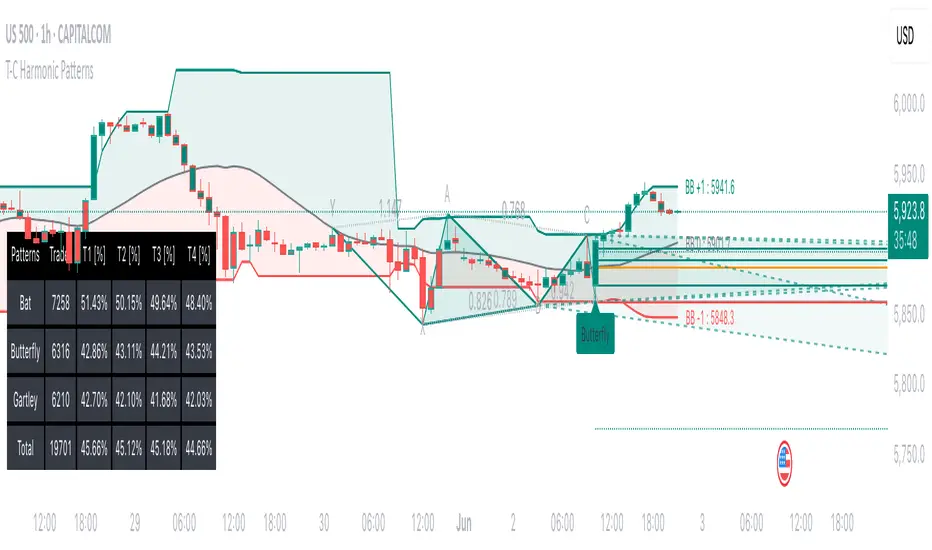
Average Trend with Deviation BandsTL,DR: A trend indicator with deviation bands using a modified Donchian calculation
This indicator plots a trend using the average of the lowest and highest closing price and the lowest low and highest high of a given period. This is similar to Donchian channels which use an average of the lowest and highest value (of a given period). This might sound like a small change but imho it provides a better "average" when lows/highs and lowest/highest closing prices are considered in the average calculation as well.
I also added the option to show 2 deviation bands (one is deactivated by default but can be activated in the options menu). The deviation band uses the standard deviation (of the average trend) and can be used to determine if a price movement is still in a "normal" range or not. Based on my testing it is fine to use one band with a standard deviation of 1 but it is also possible to show a second band with a different deviation value if needed. The bands (and trendline) can also be used as dynamic support/resistance zones.
Trendline without deviation bands
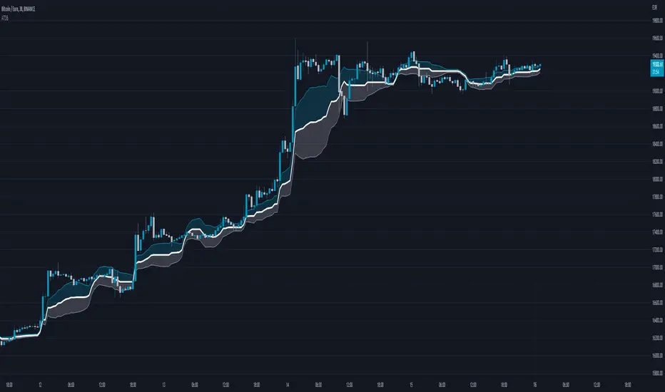
Moving Average Compendium RefurbishedThis is my effort to bring together in a single script the widest range of moving averages possible.
I aggregated the calculation of averages within a library.
For more information about the library follow the link:
Basically this indicator is the visual result of this library.
You can choose the moving average and the script updates the chart as per the type.
The unique parameters of certain moving averages remain at their default values.
To have a rainbow of moving averages I also made an indicator:
Available moving averages:
AARMA = 'Adaptive Autonomous Recursive Moving Average'
ADEMA = '* Alpha-Decreasing Exponential Moving Average'
AHMA = 'Ahrens Moving Average'
ALMA = 'Arnaud Legoux Moving Average'
ALSMA = 'Adaptive Least Squares'
AUTOL = 'Auto-Line'
CMA = 'Corrective Moving average'
CORMA = 'Correlation Moving Average Price'
COVWEMA = 'Coefficient of Variation Weighted Exponential Moving Average'
COVWMA = 'Coefficient of Variation Weighted Moving Average'
DEMA = 'Double Exponential Moving Average'
DONCHIAN = 'Donchian Middle Channel'
EDMA = 'Exponentially Deviating Moving Average'
EDSMA = 'Ehlers Dynamic Smoothed Moving Average'
EFRAMA = '* Ehlrs Modified Fractal Adaptive Moving Average'
EHMA = 'Exponential Hull Moving Average'
EMA = 'Exponential Moving Average'
EPMA = 'End Point Moving Average'
ETMA = 'Exponential Triangular Moving Average'
EVWMA = 'Elastic Volume Weighted Moving Average'
FAMA = 'Following Adaptive Moving Average'
FIBOWMA = 'Fibonacci Weighted Moving Average'
FISHLSMA = 'Fisher Least Squares Moving Average'
FRAMA = 'Fractal Adaptive Moving Average'
GMA = 'Geometric Moving Average'
HKAMA = 'Hilbert based Kaufman\'s Adaptive Moving Average'
HMA = 'Hull Moving Average'
JURIK = 'Jurik Moving Average'
KAMA = 'Kaufman\'s Adaptive Moving Average'
LC_LSMA = '1LC-LSMA (1 line code lsma with 3 functions)'
LEOMA = 'Leo Moving Average'
LINWMA = 'Linear Weighted Moving Average'
LSMA = 'Least Squares Moving Average'
MAMA = 'MESA Adaptive Moving Average'
MCMA = 'McNicholl Moving Average'
MEDIAN = 'Median'
REGMA = 'Regularized Exponential Moving Average'
REMA = 'Range EMA'
REPMA = 'Repulsion Moving Average'
RMA = 'Relative Moving Average'
RSIMA = 'RSI Moving average'
RVWAP = '* Rolling VWAP'
SMA = 'Simple Moving Average'
SMMA = 'Smoothed Moving Average'
SRWMA = 'Square Root Weighted Moving Average'
SW_MA = 'Sine-Weighted Moving Average'
SWMA = '* Symmetrically Weighted Moving Average'
TEMA = 'Triple Exponential Moving Average'
THMA = 'Triple Hull Moving Average'
TREMA = 'Triangular Exponential Moving Average'
TRSMA = 'Triangular Simple Moving Average'
TT3 = 'Tillson T3'
VAMA = 'Volatility Adjusted Moving Average'
VIDYA = 'Variable Index Dynamic Average'
VWAP = '* VWAP'
VWMA = 'Volume-weighted Moving Average'
WMA = 'Weighted Moving Average'
WWMA = 'Welles Wilder Moving Average'
XEMA = 'Optimized Exponential Moving Average'
ZEMA = 'Zero-Lag Exponential Moving Average'
ZSMA = 'Zero-Lag Simple Moving Average'
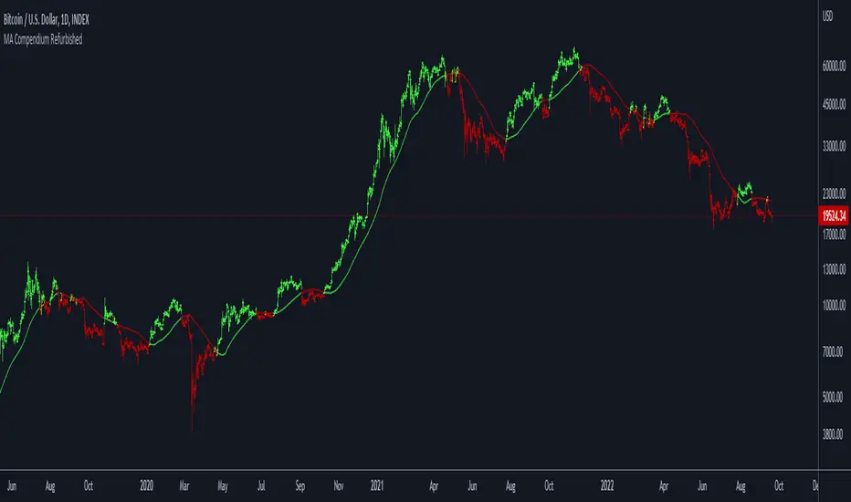
Moving Averages ProxyLibrary "MovingAveragesProxy"
Moving Averages Proxy - Library of all moving averages spread out in different libraries
rvwap(_src, fixedTfInput, minsInput, hoursInput, daysInput, minBarsInput)
Calculates the Rolling VWAP (customized VWAP developed by the team of TradingView)
Parameters:
_src : (float) Source. Default: close
fixedTfInput : (bool) Use a fixed time period. Default: false
minsInput : (int) Minutes. Default: 0
hoursInput : (int) Hours. Default: 0
daysInput : (int) Days. Default: 1
minBarsInput : (int) Bars. Default: 10
Returns: (float) Rolling VWAP
correlationMa(src, len, factor)
Correlation Moving Average
Parameters:
src : (float) Source. Default: close
len : (int) Length
factor : (float) Factor. Default: 1.7
Returns: (float) Correlation Moving Average
regma(src, len, lambda)
Regularized Exponential Moving Average
Parameters:
src : (float) Source. Default: close
len : (int) Length
lambda : (float) Lambda. Default: 0.5
Returns: (float) Regularized Exponential Moving Average
repma(src, len)
Repulsion Moving Average
Parameters:
src : (float) Source. Default: close
len : (int) Length
Returns: (float) Repulsion Moving Average
epma(src, length, offset)
End Point Moving Average
Parameters:
src : (float) Source. Default: close
length : (int) Length
offset : (float) Offset. Default: 4
Returns: (float) End Point Moving Average
lc_lsma(src, length)
1LC-LSMA (1 line code lsma with 3 functions)
Parameters:
src : (float) Source. Default: close
length : (int) Length
Returns: (float) 1LC-LSMA Moving Average
aarma(src, length)
Adaptive Autonomous Recursive Moving Average
Parameters:
src : (float) Source. Default: close
length : (int) Length
Returns: (float) Adaptive Autonomous Recursive Moving Average
alsma(src, length)
Adaptive Least Squares
Parameters:
src : (float) Source. Default: close
length : (int) Length
Returns: (float) Adaptive Least Squares
ahma(src, length)
Ahrens Moving Average
Parameters:
src : (float) Source. Default: close
length : (int) Length
Returns: (float) Ahrens Moving Average
adema(src)
Ahrens Moving Average
Parameters:
src : (float) Source. Default: close
Returns: (float) Moving Average
autol(src, lenDev)
Auto-Line
Parameters:
src : (float) Source. Default: close
lenDev : (int) Length for standard deviation
Returns: (float) Auto-Line
fibowma(src, length)
Fibonacci Weighted Moving Average
Parameters:
src : (float) Source. Default: close
length : (int) Length
Returns: (float) Moving Average
fisherlsma(src, length)
Fisher Least Squares Moving Average
Parameters:
src : (float) Source. Default: close
length : (int) Length
Returns: (float) Moving Average
leoma(src, length)
Leo Moving Average
Parameters:
src : (float) Source. Default: close
length : (int) Length
Returns: (float) Moving Average
linwma(src, period, weight)
Linear Weighted Moving Average
Parameters:
src : (float) Source. Default: close
period : (int) Length
weight : (int) Weight
Returns: (float) Moving Average
mcma(src, length)
McNicholl Moving Average
Parameters:
src : (float) Source. Default: close
length : (int) Length
Returns: (float) Moving Average
srwma(src, length)
Square Root Weighted Moving Average
Parameters:
src : (float) Source. Default: close
length : (int) Length
Returns: (float) Moving Average
EDSMA(src, len)
Ehlers Dynamic Smoothed Moving Average.
Parameters:
src : Series to use ('close' is used if no argument is supplied).
len : Lookback length to use.
Returns: EDSMA smoothing.
dema(x, t)
Double Exponential Moving Average.
Parameters:
x : Series to use ('close' is used if no argument is supplied).
t : Lookback length to use.
Returns: DEMA smoothing.
tema(src, len)
Triple Exponential Moving Average.
Parameters:
src : Series to use ('close' is used if no argument is supplied).
len : Lookback length to use.
Returns: TEMA smoothing.
smma(src, len)
Smoothed Moving Average.
Parameters:
src : Series to use ('close' is used if no argument is supplied).
len : Lookback length to use.
Returns: SMMA smoothing.
hullma(src, len)
Hull Moving Average.
Parameters:
src : Series to use ('close' is used if no argument is supplied).
len : Lookback length to use.
Returns: Hull smoothing.
frama(x, t)
Fractal Reactive Moving Average.
Parameters:
x : Series to use ('close' is used if no argument is supplied).
t : Lookback length to use.
Returns: FRAMA smoothing.
kama(x, t)
Kaufman's Adaptive Moving Average.
Parameters:
x : Series to use ('close' is used if no argument is supplied).
t : Lookback length to use.
Returns: KAMA smoothing.
vama(src, len)
Volatility Adjusted Moving Average.
Parameters:
src : Series to use ('close' is used if no argument is supplied).
len : Lookback length to use.
Returns: VAMA smoothing.
donchian(len)
Donchian Calculation.
Parameters:
len : Lookback length to use.
Returns: Average of the highest price and the lowest price for the specified look-back period.
Jurik(src, len)
Jurik Moving Average.
Parameters:
src : Series to use ('close' is used if no argument is supplied).
len : Lookback length to use.
Returns: JMA smoothing.
xema(src, len)
Optimized Exponential Moving Average.
Parameters:
src : Series to use ('close' is used if no argument is supplied).
len : Lookback length to use.
Returns: XEMA smoothing.
ehma(src, len)
EHMA - Exponential Hull Moving Average
Parameters:
src : Source
len : Period
Returns: Exponential Hull Moving Average (EHMA)
covwema(src, len)
Coefficient of Variation Weighted Exponential Moving Average (COVWEMA)
Parameters:
src : Source
len : Period
Returns: Coefficient of Variation Weighted Exponential Moving Average (COVWEMA)
covwma(src, len)
Coefficient of Variation Weighted Moving Average (COVWMA)
Parameters:
src : Source
len : Period
Returns: Coefficient of Variation Weighted Moving Average (COVWMA)
eframa(src, len, FC, SC)
Ehlrs Modified Fractal Adaptive Moving Average (EFRAMA)
Parameters:
src : Source
len : Period
FC : Lower Shift Limit for Ehlrs Modified Fractal Adaptive Moving Average
SC : Upper Shift Limit for Ehlrs Modified Fractal Adaptive Moving Average
Returns: Ehlrs Modified Fractal Adaptive Moving Average (EFRAMA)
etma(src, len)
Exponential Triangular Moving Average (ETMA)
Parameters:
src : Source
len : Period
Returns: Exponential Triangular Moving Average (ETMA)
rma(src, len)
RMA - RSI Moving average
Parameters:
src : Source
len : Period
Returns: RSI Moving average (RMA)
thma(src, len)
THMA - Triple Hull Moving Average
Parameters:
src : Source
len : Period
Returns: Triple Hull Moving Average (THMA)
vidya(src, len)
Variable Index Dynamic Average (VIDYA)
Parameters:
src : Source
len : Period
Returns: Variable Index Dynamic Average (VIDYA)
zsma(src, len)
Zero-Lag Simple Moving Average (ZSMA)
Parameters:
src : Source
len : Period
Returns: Zero-Lag Simple Moving Average (ZSMA)
zema(src, len)
Zero-Lag Exponential Moving Average (ZEMA)
Parameters:
src : Source
len : Period
Returns: Zero-Lag Exponential Moving Average (ZEMA)
evwma(src, len)
EVWMA - Elastic Volume Weighted Moving Average
Parameters:
src : Source
len : Period
Returns: Elastic Volume Weighted Moving Average (EVWMA)
tt3(src, len, a1_t3)
Tillson T3
Parameters:
src : Source
len : Period
a1_t3 : Tillson T3 Volume Factor
Returns: Tillson T3
gma(src, len)
GMA - Geometric Moving Average
Parameters:
src : Source
len : Period
Returns: Geometric Moving Average (GMA)
wwma(src, len)
WWMA - Welles Wilder Moving Average
Parameters:
src : Source
len : Period
Returns: Welles Wilder Moving Average (WWMA)
cma(src, len)
Corrective Moving average (CMA)
Parameters:
src : Source
len : Period
Returns: Corrective Moving average (CMA)
edma(src, len)
Exponentially Deviating Moving Average (MZ EDMA)
Parameters:
src : Source
len : Period
Returns: Exponentially Deviating Moving Average (MZ EDMA)
rema(src, len)
Range EMA (REMA)
Parameters:
src : Source
len : Period
Returns: Range EMA (REMA)
sw_ma(src, len)
Sine-Weighted Moving Average (SW-MA)
Parameters:
src : Source
len : Period
Returns: Sine-Weighted Moving Average (SW-MA)
mama(src, len)
MAMA - MESA Adaptive Moving Average
Parameters:
src : Source
len : Period
Returns: MESA Adaptive Moving Average (MAMA)
fama(src, len)
FAMA - Following Adaptive Moving Average
Parameters:
src : Source
len : Period
Returns: Following Adaptive Moving Average (FAMA)
hkama(src, len)
HKAMA - Hilbert based Kaufman's Adaptive Moving Average
Parameters:
src : Source
len : Period
Returns: Hilbert based Kaufman's Adaptive Moving Average (HKAMA)
getMovingAverage(type, src, len, lsmaOffset, inputAlmaOffset, inputAlmaSigma, FC, SC, a1_t3, fixedTfInput, daysInput, hoursInput, minsInput, minBarsInput, lambda, volumeWeighted, gamma_aarma, smooth, linweight, volatility_lookback, jurik_phase, jurik_power)
Abstract proxy function that invokes the calculation of a moving average according to type
Parameters:
type : (string) Type of moving average
src : (float) Source of series (close, high, low, etc.)
len : (int) Period of loopback to calculate the average
lsmaOffset : (int) Offset for Least Squares MA
inputAlmaOffset : (float) Offset for ALMA
inputAlmaSigma : (float) Sigma for ALMA
FC : (int) Lower Shift Limit for Ehlrs Modified Fractal Adaptive Moving Average
SC : (int) Upper Shift Limit for Ehlrs Modified Fractal Adaptive Moving Average
a1_t3 : (float) Tillson T3 Volume Factor
fixedTfInput : (bool) Use a fixed time period in Rolling VWAP
daysInput : (int) Days in Rolling VWAP
hoursInput : (int) Hours in Rolling VWAP
minsInput : (int) Minutrs in Rolling VWAP
minBarsInput : (int) Bars in Rolling VWAP
lambda : (float) Regularization Constant in Regularized EMA
volumeWeighted : (bool) Apply volume weighted calculation in selected moving average
gamma_aarma : (float) Gamma for Adaptive Autonomous Recursive Moving Average
smooth : (float) Smooth for Adaptive Least Squares
linweight : (float) Weight for Volume Weighted Moving Average
volatility_lookback : (int) Loopback for Volatility Adjusted Moving Average
jurik_phase : (int) Phase for Jurik Moving Average
jurik_power : (int) Power for Jurik Moving Average
Returns: (float) Moving average
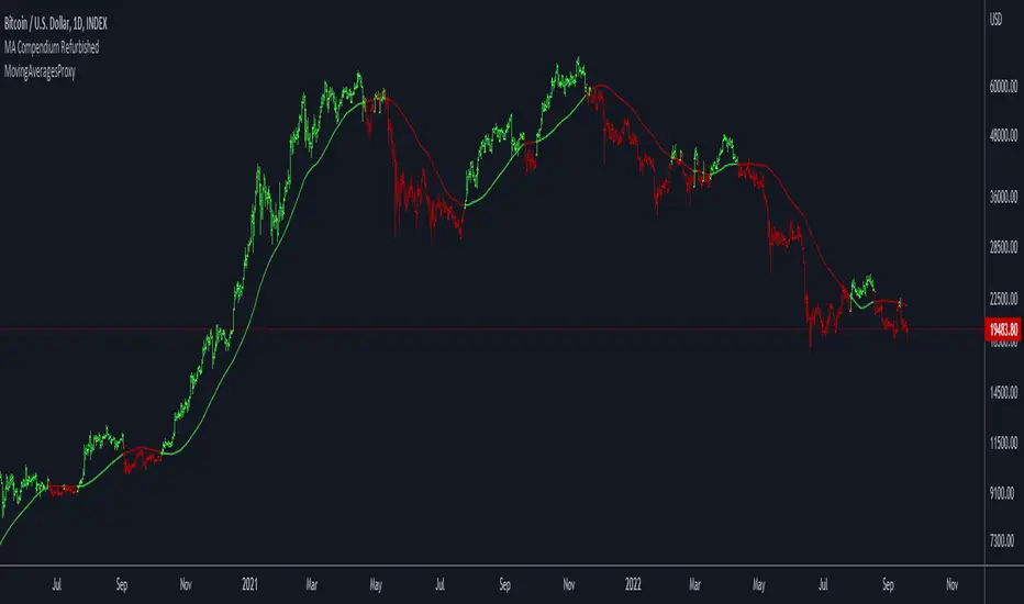
1 Indicator to rule them allThe best combination indicator consisting of 4 SMA's, 4 EMA's, Donchian Channels, Parabolic SAR, Bollinger Bands, Ichimoku Cloud, a trend strength highlight for the bollinger bands background according to the ADX, labels on the chart to draw in when the Directional Index plus and minus cross, and a background highlight for low and high volatility according to the Historical Volatility Percentile.
The Indicators and placed and group intentionally, with the SMA and EMA's next to the Donchian Channels to draw in areas of support and resistance, with the parabolic SAR afterwards for confirmation on entries and exits.
Next are the Bollinger Bands and the Ichimoku cloud, which when used in combination by an experienced trader allows one to see the trend and spot any developing opportunities at a glance. These can be used in combination with the ADX background in the bolls to point out when trends start and end.
The Directional Indexes crossing implies a equilibrium point has been reached between the buy and selling pressure. Finally the background highlight according to low and high periods of volatility does well to ensure you're entering into the best trades at the best times.
These indicators used together in combo with momentum oscillators will lead to a full and complete picture of the trend and the most likely places for future price to come, allowing a holistic view and confluence between different, noncollinear indicators to paint occam's razor onto the charts.
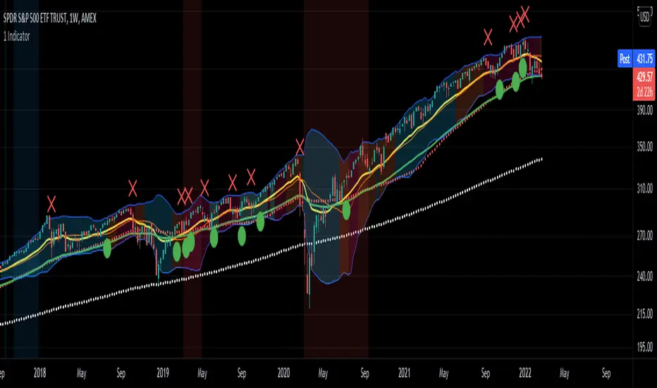
historicalrangeLibrary "historicalrange"
Library provices a method to calculate historical percentile range of series.
hpercentrank(source) calculates historical percentrank of the source
Parameters:
source : Source for which historical percentrank needs to be calculated. Source should be ranging between 0-100. If using a source which can beyond 0-100, use short term percentrank to baseline them.
Returns: pArray - percentrank array which contains how many instances of source occurred at different levels.
upperPercentile - percentile based on higher value
lowerPercentile - percentile based on lower value
median - median value of the source
max - max value of the source
distancefromath(source) returns stats on historical distance from ath in terms of percentage
Parameters:
source : for which stats are calculated
Returns: percentile and related historical stats regarding distance from ath
distancefromma(maType, length, source) returns stats on historical distance from moving average in terms of percentage
Parameters:
maType : Moving Average Type : Can be sma, ema, hma, rma, wma, vwma, swma, highlow, linreg, median
length : Moving Average Length
source : for which stats are calculated
Returns: percentile and related historical stats regarding distance from ath
bpercentb(source, maType, length, multiplier, sticky) returns percentrank and stats on historical bpercentb levels
Parameters:
source : Moving Average Source
maType : Moving Average Type : Can be sma, ema, hma, rma, wma, vwma, swma, highlow, linreg, median
length : Moving Average Length
multiplier : Standard Deviation multiplier
sticky : - sticky boundaries which will only change when value is outside boundary.
Returns: percentile and related historical stats regarding Bollinger Percent B
kpercentk(source, maType, length, multiplier, useTrueRange, sticky) returns percentrank and stats on historical kpercentk levels
Parameters:
source : Moving Average Source
maType : Moving Average Type : Can be sma, ema, hma, rma, wma, vwma, swma, highlow, linreg, median
length : Moving Average Length
multiplier : Standard Deviation multiplier
useTrueRange : - if set to false, uses high-low.
sticky : - sticky boundaries which will only change when value is outside boundary.
Returns: percentile and related historical stats regarding Keltener Percent K
dpercentd(useAlternateSource, alternateSource, length, sticky) returns percentrank and stats on historical dpercentd levels
Parameters:
useAlternateSource : - Custom source is used only if useAlternateSource is set to true
alternateSource : - Custom source
length : - donchian channel length
sticky : - sticky boundaries which will only change when value is outside boundary.
Returns: percentile and related historical stats regarding Donchian Percent D
oscillator(type, length, shortLength, longLength, source, highSource, lowSource, method, highlowLength, sticky) oscillator - returns Choice of oscillator with custom overbought/oversold range
Parameters:
type : - oscillator type. Valid values : cci, cmo, cog, mfi, roc, rsi, stoch, tsi, wpr
length : - Oscillator length - not used for TSI
shortLength : - shortLength only used for TSI
longLength : - longLength only used for TSI
source : - custom source if required
highSource : - custom high source for stochastic oscillator
lowSource : - custom low source for stochastic oscillator
method : - Valid values for method are : sma, ema, hma, rma, wma, vwma, swma, highlow, linreg, median
highlowLength : - length on which highlow of the oscillator is calculated
sticky : - overbought, oversold levels won't change unless crossed
Returns: percentile and related historical stats regarding oscillator
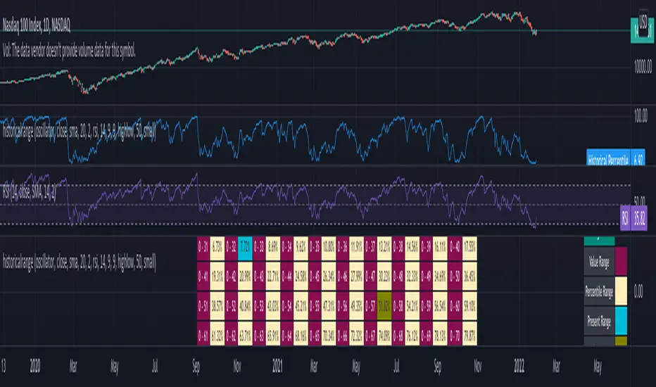
Brrrrr strategyTheory
When Tether prints new USDT the price of BTC rises.
When Tether burns USDT the price of BTC goes down.
Idea
Open a long position when Tether starts printing new USDT.
Close a long position when Tether begins to burn USDT.
Optional: open a short position.
(Short positions can be disabled in this script's settings.)
Donchian Channel
USDT changes frequently and almost every day. Therefore it is necessary to reduce the number of signals. This way there will be less false loss signals. The Donchian channel is well suited for this task.
If the amount of USDT has exceeded the maximum for the last 50 days, it is a signal to open a long position.
If the amount of USDT has become less than the minimum over the last 50 days, it is a signal to close a long position. Or to open a short position.
The number of days can be changed in the settings of this script.
Data
The data is only available for 1-day timeframe. The data provider is Glassnode.
For
Only for BTC /USD (or BTC /USDT, BTC/USDC , etc)
For 1 day timeframe only

Speed IndicatorThe indicator showcases the Speed at which the prices change based on the set length. It does not show trend direction simply because Speed is a scalar quantity. It helps to identify when the prices are racing, slowing down, or in a range.
The formula used for calculation is Speed = Total Distance Travelled / Time.
Time is the period range that can be defined to set the lookback period.
The length is calculated by finding the absolute value of the difference between the current and closing prices one period ago. The lengths are added for the defined Time, and the Total Distance Travelled by the price is calculated. The formula of 'current price' - price 'Time' periods ago is not used, which calculates the displacement of the price used in figuring the velocity .
The Speed is then calculated using the defined formula.
For example, in the last 20 days, a stock price moved a total of 15000 points, then the Speed of the price would be 750 points per day. Therefore the price is expected to be moving around 750 points, either up or down.
There is also an application of the Donchian Channels to the calculated Speed. It helps to define a dynamic range of the Speed and easily visualize if the Speed is increasing, decreasing, or being stable. The range showcases a Speedometer , hence easing the interpretation of the Speed. Speed Range can also be customized for the Donchian channel. The contraction of the channels would occur when the Speed has been steady for some time, which would mean the price has not moved out from its range.
The importance of the indicator is to identify when the prices have slowed down to enter positions safely, since entering positions during higher speeds would be like jumping onto a fast-moving train. Although, it is up to the user's risk appetite if they wish to enter during low speeds or high speeds. The basic strategy is to enter during slow speeds, hold as speed increases, exit as Speed starts to slow down for its highs. That is the basic idea but can be customized as per the user.

Double_based_emaThe indicator shows two EMA. One superior and one inferior. The prices used to generate the EMA are diferent.
For the superior EMA the price comes from the superior part of a Donchian Channel with the same period as the EMA.
For the inferior EMA the price comes from the inferior part of the same Donchian Chanell.
There is a superior limit and a inferior limit to this prices equal a 1/2 ATR with same period.
The prices from superior part are those between the center of the channel and superior channel minus 1/2 ATR.
The prices from inferior part are those between the center of the channel and inferior channel plus 1/2 ATR.
This gives a litlle gain in speed to the EMA lecture and a second point of view as the indicator shows the superior EMA when the price is above the midle and shows the inferior EMA when the price is under the midle of the channel.

TrendCalculusThis indicator makes visualising some of the core TrendCalculus algorithm's key information and features both fast and easy for casual analysis.
Interpretation:
a) The light blue channel is the lagged price channel calculated over the timeframe of your choosing for a period of N values. When the current price breaks out of this channel the previous price major high/low can be identified as a trend reversal. This helps in counting trend "waves" and is a rolling visual version of ideas I developed for counting Elliot Waves. For EW analysis, your mileage may vary depending on the asset inspected, but the chart allows you to clearly count waves on a particular scale of time (period) ignoring noise on other time scales.
b) The green/red channel is a support/resistance indicator region that shows the relationship of the current price to the key pivot points on this time scale (period) and these make for good visual indication that the current trend is up (green), or down (red). You may find them helpful for identifying breakouts and placing stops - but this was not their original intention. The pink line is the mid point of closing values in the lagged price channel, and the orange line the mid point of closing values in the current price channel.
About TrendCalculus (TC):
TC is implemented in several languages including Lua, Scala and Python. The Lua implementation is the reference and has the most advanced functionality and delivers a powerful data processing tool for both multi-scale trend reversal detection, reversal labelling, as well as trend feature production - all useful things helping it to produce training data for machine learning models that detect trend changes in real time.
This charting tool includes: (1) two consecutive lagged Donchian channels configured to a common period N, (2) the current price, and (3) the mid price of both Donchian channels. These calculations are all part of the TC codebase, and are brought to life in this charting tool.
Motivation:
By creating a TC charting tool - the machine learning model is swapped for *your eyes* and *your brain*. Using the same inputs as the machine, you can use this chart to learn to detect trend changes, and understand how time frame (long periods, short periods) affect your view of trend change. If you choose to use it to trade, or make investment decisions, do so at your own risk. This indicator does not deliver financial advice.
TrendCalculus is the invention of Andrew Morgan, author of Mastering Spark for Data Science (2017).
The original core TrendCalculus (TC) algorithm itself is published as open-source code on github under a GPL licence, and free to use and develop.