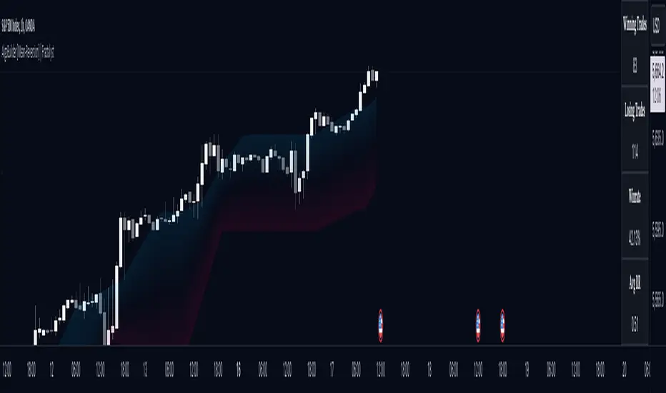
AlgoBuilder [Mean-Reversion] | FractalystWhat's the strategy's purpose and functionality?
This strategy is designed for both traders and investors looking to rely and trade based on historical and backtested data using automation.
The main goal is to build profitable mean-reversion strategies that outperform the underlying asset in terms of returns while minimizing drawdown.
For example, as for a benchmark, if the S&P 500 (SPX) has achieved an estimated 10% annual return with a maximum drawdown of -57% over the past 20 years, using this strategy with different entry and exit techniques, users can potentially seek ways to achieve a higher Compound Annual Growth Rate (CAGR) while maintaining a lower maximum drawdown.
Although the strategy can be applied to all markets and timeframes, it is most effective on stocks, indices, future markets, cryptocurrencies, and commodities and JPY currency pairs given their trending behaviors.
In trending market conditions, the strategy employs a combination of moving averages and diverse entry models to identify and capitalize on upward market movements. It integrates market structure-based moving averages and bands mechanisms across different timeframes and provides exit techniques, including percentage-based and risk-reward (RR) based take profit levels.
Additionally, the strategy has also a feature that includes a built-in probability function for traders who want to implement probabilities right into their trading strategies.
Performance summary, weekly, and monthly tables enable quick visualization of performance metrics like net profit, maximum drawdown, profit factor, average trade, average risk-reward ratio (RR), and more.
This aids optimization to meet specific goals and risk tolerance levels effectively.
-----
How does the strategy perform for both investors and traders?
The strategy has two main modes, tailored for different market participants: Traders and Investors.
Trading:
1. Trading:
- Designed for traders looking to capitalize on bullish trending markets.
- Utilizes a percentage risk per trade to manage risk and optimize returns.
- Suitable for active trading with a focus on mean-reversion and risk per trade approach.
◓: Mode | %: Risk percentage per trade
3. Investing:
- Geared towards investors who aim to capitalize on bullish trending markets without using leverage while mitigating the asset's maximum drawdown.
- Utilizes pre-define percentage of the equity to buy, hold, and manage the asset.
- Focuses on long-term growth and capital appreciation by fully investing in the asset during bullish conditions.
- ◓: Mode | %: Risk not applied (In investing mode, the strategy uses 10% of equity to buy the asset)
-----
What's is FRMA? How does the triple bands work? What are the underlying calculations?
Middle Band (FRMA):
The middle band is the core of the FRMA system. It represents the Fractalyst Moving Average, calculated by identifying the most recent external swing highs and lows in the market structure.
By determining these external swing pivot points, which act as significant highs and lows within the market range, the FRMA provides a unique moving average that adapts to market structure changes.
Upper Band:
The upper band shows the average price of the most recent external swing highs.
External swing highs are identified as the highest points between pivot points in the market structure.
This band helps traders identify potential overbought conditions when prices approach or exceed this upper band.
Lower Band:
The lower band shows the average price of the most recent external swing lows.
External swing lows are identified as the lowest points between pivot points in the market structure.
The script utilizes this band to identify potential oversold conditions, triggering entry signals as prices approach or drop below the lower band.
Adjustments Based on User Inputs:
Users can adjust how the upper and lower bands are calculated based on their preferences:
Upper/Lower: This method calculates the average bands using the prices of external swing highs and lows identified in the market.
Percentage Deviation from FRMA: Alternatively, users can opt to calculate the bands based on a percentage deviation from the middle FRMA. This approach provides flexibility to adjust the width of the bands relative to market conditions and volatility.
-----
What's the purpose of using moving averages in this strategy? What are the underlying calculations?
Using moving averages is a widely-used technique to trade with the trend.
The main purpose of using moving averages in this strategy is to filter out bearish price action and to only take trades when the price is trading ABOVE specified moving averages.
The script uses different types of moving averages with user-adjustable timeframes and periods/lengths, allowing traders to try out different variations to maximize strategy performance and minimize drawdowns.
By applying these calculations, the strategy effectively identifies bullish trends and avoids market conditions that are not conducive to profitable trades.
The MA filter allows traders to choose whether they want a specific moving average above or below another one as their entry condition.
This comparison filter can be turned on (>) or off.
For example, you can set the filter so that MA#1 > MA#2, meaning the first moving average must be above the second one before the script looks for entry conditions. This adds an extra layer of trend confirmation, ensuring that trades are only taken in more favorable market conditions.
⍺: MA Period | Σ: MA Timeframe
-----
What entry modes are used in this strategy? What are the underlying calculations?
The strategy by default uses two different techniques for the entry criteria with user-adjustable left and right bars: Breakout and Fractal.
1. Breakout Entries :
- The strategy looks for pivot high points with a default period of 3.
- It stores the most recent high level in a variable.
- When the price crosses above this most recent level, the strategy checks if all conditions are met and the bar is closed before taking the buy entry.
◧: Pivot high left bars period | ◨: Pivot high right bars period
2. Fractal Entries :
- The strategy looks for pivot low points with a default period of 3.
- When a pivot low is detected, the strategy checks if all conditions are met and the bar is closed before taking the buy entry.
◧: Pivot low left bars period | ◨: Pivot low right bars period
2. Hunt Entries :
- The strategy identifies a candle that wicks through the lower FRMA band.
- It waits for the next candle to close above the low of the wick candle.
- When this condition is met and the bar is closed, the strategy takes the buy entry.
By utilizing these entry modes, the strategy aims to capitalize on bullish price movements while ensuring that the necessary conditions are met to validate the entry points.
-----
What type of stop-loss identification method are used in this strategy? What are the underlying calculations?
Initial Stop-Loss:
1. ATR Based:
The Average True Range (ATR) is a method used in technical analysis to measure volatility. It is not used to indicate the direction of price but to measure volatility, especially volatility caused by price gaps or limit moves.
Calculation:
- To calculate the ATR, the True Range (TR) first needs to be identified. The TR takes into account the most current period high/low range as well as the previous period close.
The True Range is the largest of the following:
- Current Period High minus Current Period Low
- Absolute Value of Current Period High minus Previous Period Close
- Absolute Value of Current Period Low minus Previous Period Close
- The ATR is then calculated as the moving average of the TR over a specified period. (The default period is 14).
Example - ATR (14) * 2
⍺: ATR period | Σ: ATR Multiplier
2. ADR Based:
The Average Day Range (ADR) is an indicator that measures the volatility of an asset by showing the average movement of the price between the high and the low over the last several days.
Calculation:
- To calculate the ADR for a particular day:
- Calculate the average of the high prices over a specified number of days.
- Calculate the average of the low prices over the same number of days.
- Find the difference between these average values.
- The default period for calculating the ADR is 14 days. A shorter period may introduce more noise, while a longer period may be slower to react to new market movements.
Example - ADR (20) * 2
⍺: ADR period | Σ: ADR Multiplier
3. PL Based:
This method places the stop-loss at the low of the previous candle.
If the current entry is based on the hunt entry strategy, the stop-loss will be placed at the low of the candle that wicks through the lower FRMA band.
Example:
If the previous candle's low is 100, then the stop-loss will be set at 100.
This method ensures the stop-loss is placed just below the most recent significant low, providing a logical and immediate level for risk management.
Application in Strategy (ATR/ADR):
- The strategy calculates the current bar's ADR/ATR with a user-defined period.
- It then multiplies the ADR/ATR by a user-defined multiplier to determine the initial stop-loss level.
By using these methods, the strategy dynamically adjusts the initial stop-loss based on market volatility, helping to protect against adverse price movements while allowing for enough room for trades to develop.
Each market behaves differently across various timeframes, and it is essential to test different parameters and optimizations to find out which trailing stop-loss method gives you the desired results and performance.
-----
What type of break-even and take profit identification methods are used in this strategy? What are the underlying calculations?
For Break-Even:
Percentage (%) Based:
Moves the initial stop-loss to the entry price when the price reaches a certain percentage above the entry.
Calculation:
Break-even level = Entry Price * (1 + Percentage / 100)
Example:
If the entry price is $100 and the break-even percentage is 5%, the break-even level is $100 * 1.05 = $105.
Risk-to-Reward (RR) Based:
Moves the initial stop-loss to the entry price when the price reaches a certain RR ratio.
Calculation:
Break-even level = Entry Price + (Initial Risk * RR Ratio)
Example:
If the entry price is $100, the initial risk is $10, and the RR ratio is 2, the break-even level is $100 + ($10 * 2) = $120.
FRMA Based:
Moves the stop-loss to break-even when the price hits the FRMA level at which the entry was taken.
Calculation:
Break-even level = FRMA level at the entry
Example:
If the FRMA level at entry is $102, the break-even level is set to $102 when the price reaches $102.
For TP1 (Take Profit 1):
- You can choose to set a take profit level at which your position gets fully closed or 50% if the TP2 boolean is enabled.
- Similar to break-even, you can select either a percentage (%) or risk-to-reward (RR) based take profit level, allowing you to set your TP1 level as a percentage amount above the entry price or based on RR.
For TP2 (Take Profit 2):
- You can choose to set a take profit level at which your position gets fully closed.
- As with break-even and TP1, you can select either a percentage (%) or risk-to-reward (RR) based take profit level, allowing you to set your TP2 level as a percentage amount above the entry price or based on RR.
When Both Percentage (%) Based and RR Based Take Profit Levels Are Off:
The script will adjust the take profit level to the higher FRMA band set within user inputs.
Calculation:
Take profit level = Higher FRMA band length/timeframe specified by the user.
This ensures that when neither percentage-based nor risk-to-reward-based take profit methods are enabled, the strategy defaults to using the higher FRMA band as the take profit level, providing a consistent and structured approach to profit-taking.
For TP1 and TP2, it's specifying the price levels at which the position is partially or fully closed based on the chosen method (percentage or RR) above the entry price.
These calculations are crucial for managing risk and optimizing profitability in the strategy.
⍺: BE/TP type (%/RR) | Σ: how many RR/% above the current price
-----
What's the ADR filter? What does it do? What are the underlying calculations?
The Average Day Range (ADR) measures the volatility of an asset by showing the average movement of the price between the high and the low over the last several days.
The period of the ADR filter used in this strategy is tied to the same period you've used for your initial stop-loss.
Users can define the minimum ADR they want to be met before the script looks for entry conditions.
ADR Bias Filter:
- Compares the current bar ADR with the ADR (Defined by user):
- If the current ADR is higher, it indicates that volatility has increased compared to ADR (DbU).(⬆)
- If the current ADR is lower, it indicates that volatility has decreased compared to ADR (DbU).(⬇)
Calculations:
1. Calculate ADR:
- Average the high prices over the specified period.
- Average the low prices over the same period.
- Find the difference between these average values in %.
2. Current ADR vs. ADR (DbU):
- Calculate the ADR for the current bar.
- Calculate the ADR (DbU).
- Compare the two values to determine if volatility has increased or decreased.
By using the ADR filter, the strategy ensures that trades are only taken in favorable market conditions where volatility meets the user's defined threshold, thus optimizing entry conditions and potentially improving the overall performance of the strategy.
>: Minimum required ADR for entry | %: Current ADR comparison to ADR of 14 days ago.
-----
What's the probability filter? What are the underlying calculations?
The probability filter is designed to enhance trade entries by using buyside liquidity and probability analysis to filter out unfavorable conditions.
This filter helps in identifying optimal entry points where the likelihood of a profitable trade is higher.
Calculations:
1. Understanding Swing highs and Swing Lows
Swing High: A Swing High is formed when there is a high with 2 lower highs to the left and right.
Swing Low: A Swing Low is formed when there is a low with 2 higher lows to the left and right.
2. Understanding the purpose and the underlying calculations behind Buyside, Sellside and Equilibrium levels.
3. Understanding probability calculations
1. Upon the formation of a new range, the script waits for the price to reach and tap into equilibrium or the 50% level. Status: "⏸" - Inactive
2. Once equilibrium is tapped into, the equilibrium status becomes activated and it waits for either liquidity side to be hit. Status: "▶" - Active
3. If the buyside liquidity is hit, the script adds to the count of successful buyside liquidity occurrences. Similarly, if the sellside is tapped, it records successful sellside liquidity occurrences.
5. Finally, the number of successful occurrences for each side is divided by the overall count individually to calculate the range probabilities.
Note: The calculations are performed independently for each directional range. A range is considered bearish if the previous breakout was through a sellside liquidity. Conversely, a range is considered bullish if the most recent breakout was through a buyside liquidity.
Example - BSL > 55%
-----
What's the range length Filter? What are the underlying calculations?
The range length filter identifies the price distance between buyside and sellside liquidity levels in percentage terms. When enabled, the script only looks for entries when the minimum range length is met. This helps ensure that trades are taken in markets with sufficient price movement.
Calculations:
Range Length (%) = ( ( Buyside Level − Sellside Level ) / Current Price ) ×100
Range Bias Identification:
Bullish Bias: The current range price has broken above the previous external swing high.
Bearish Bias: The current range price has broken below the previous external swing low.
Example - Range length filter is enabled | Range must be above 1%
>: Minimum required range length for entry | %: Current range length percentage in a (Bullish/Bearish) range
-----
What's the day filter Filter, what does it do?
The day filter allows users to customize the session time and choose the specific days they want to include in the strategy session. This helps traders tailor their strategies to particular trading sessions or days of the week when they believe the market conditions are more favorable for their trading style.
Customize Session Time:
Users can define the start and end times for the trading session.
This allows the strategy to only consider trades within the specified time window, focusing on periods of higher market activity or preferred trading hours.
Select Days:
Users can select which days of the week to include in the strategy.
This feature is useful for excluding days with historically lower volatility or unfavorable trading conditions (e.g., Mondays or Fridays).
Benefits:
Focus on Optimal Trading Periods:
By customizing session times and days, traders can focus on periods when the market is more likely to present profitable opportunities.
Avoid Unfavorable Conditions:
Excluding specific days or times can help avoid trading during periods of low liquidity or high unpredictability, such as major news events or holidays.
Increased Flexibility: The filter provides increased flexibility, allowing traders to adapt the strategy to their specific needs and preferences.
Example - Day filter | Session Filter
θ: Session time | Exchange time-zone
-----
What tables are available in this script?
Table Type:
- Summary: Provides a general overview, displaying key performance parameters such as Net Profit, Profit Factor, Max Drawdown, Average Trade, Closed Trades and more.
Avg Trade: The sum of money gained or lost by the average trade generated by a strategy. Calculated by dividing the Net Profit by the overall number of closed trades. An important value since it must be large enough to cover the commission and slippage costs of trading the strategy and still bring a profit.
MaxDD: Displays the largest drawdown of losses, i.e., the maximum possible loss that the strategy could have incurred among all of the trades it has made. This value is calculated separately for every bar that the strategy spends with an open position.
Profit Factor: The amount of money a trading strategy made for every unit of money it lost (in the selected currency). This value is calculated by dividing gross profits by gross losses.
Avg RR: This is calculated by dividing the average winning trade by the average losing trade. This field is not a very meaningful value by itself because it does not take into account the ratio of the number of winning vs losing trades, and strategies can have different approaches to profitability. A strategy may trade at every possibility in order to capture many small profits, yet have an average losing trade greater than the average winning trade. The higher this value is, the better, but it should be considered together with the percentage of winning trades and the net profit.
Winrate: The percentage of winning trades generated by a strategy. Calculated by dividing the number of winning trades by the total number of closed trades generated by a strategy. Percent profitable is not a very reliable measure by itself. A strategy could have many small winning trades, making the percent profitable high with a small average winning trade, or a few big winning trades accounting for a low percent profitable and a big average winning trade. Most mean-reversion successful strategies have a percent profitability of 40-80% but are profitable due to risk management control.
BE Trades: Number of break-even trades, excluding commission/slippage.
Losing Trades: The total number of losing trades generated by the strategy.
Winning Trades: The total number of winning trades generated by the strategy.
Total Trades: Total number of taken traders visible your charts.
Net Profit: The overall profit or loss (in the selected currency) achieved by the trading strategy in the test period. The value is the sum of all values from the Profit column (on the List of Trades tab), taking into account the sign.
- Monthly: Displays performance data on a month-by-month basis, allowing users to analyze performance trends over each month.
- Weekly: Displays performance data on a week-by-week basis, helping users to understand weekly performance variations.
- OFF: Hides the performance table.
Profit Color:
- Allows users to set the color for representing profit in the performance table, helping to quickly distinguish profitable periods.
Loss Color:
- Allows users to set the color for representing loss in the performance table, helping to quickly identify loss-making periods.
These customizable tables provide traders with flexible and detailed performance analysis, aiding in better strategy evaluation and optimization.
-----
User-input styles and customizations:
To facilitate studying historical data, all conditions and rules can be applied to your charts. By plotting background colors on your charts, you'll be able to identify what worked and what didn't in certain market conditions.
Please note that all background colors in the style are disabled by default to enhance visualization.
-----
How to Use This Algobuilder to Create a Profitable Edge and System:
Choose Your Strategy mode:
- Decide whether you are creating an investing strategy or a trading strategy.
Select a Market:
- Choose a one-sided market such as stocks, indices, or cryptocurrencies.
Historical Data:
- Ensure the historical data covers at least 10 years of price action for robust backtesting.
Timeframe Selection:
- Choose the timeframe you are comfortable trading with. It is strongly recommended to use a timeframe above 15 minutes to minimize the impact of commissions/slippage on your profits.
Set Commission and Slippage:
- Properly set the commission and slippage in the strategy properties according to your broker or prop firm specifications.
Parameter Optimization:
- Use trial and error to test different parameters until you find the performance results you are looking for in the summary table or, preferably, through deep backtesting using the strategy tester.
Trade Count:
- Ensure the number of trades is 100 or more; the higher, the better for statistical significance.
Positive Average Trade:
- Make sure the average trade value is above zero.
(An important value since it must be large enough to cover the commission and slippage costs of trading the strategy and still bring a profit.)
Performance Metrics:
- Look for a high profit factor, and net profit with minimum drawdown.
- Ideally, aim for a drawdown under 20-30%, depending on your risk tolerance.
Refinement and Optimization:
- Try out different markets and timeframes.
- Continue working on refining your edge using the available filters and components to further optimize your strategy.
Automation:
- Once you’re confident in your strategy, you can use the automation section to connect the algorithm to your broker or prop firm.
- Trade a fully automated and backtested trading strategy, allowing for hands-free execution and management.
-----
What makes this strategy original?
1. Incorporating direct integration of probabilities into the strategy.
2. Utilizing built-in market structure-based moving averages across various timeframes.
4. Offering both investing and trading strategies, facilitating optimization from different perspectives.
5. Automation for efficient execution.
6. Providing a summary table for instant access to key parameters of the strategy.
-----
How to use automation?
For Traders:
1. Ensure the strategy parameters are properly set based on your optimized parameters.
2. Enter your PineConnector License ID in the designated field.
3. Specify the desired risk level.
4. Provide the Metatrader symbol.
5. Check for chart updates to ensure the automation table appears on the top right corner, displaying your License ID, risk, and symbol.
6. Set up an alert with the strategy selected as Condition and the Message as {{strategy.order.alert_message}}.
7. Activate the Webhook URL in the Notifications section, setting it as the official PineConnector webhook address.
8. Double-check all settings on PineConnector to ensure the connection is successful.
9. Create the alert for entry/exit automation.
For Investors:
1. Ensure the strategy parameters are properly set based on your optimized parameters.
2. Choose "Investing" in the user-input settings.
3. Create an alert with a specified name.
4. Customize the notifications tab to receive alerts via email.
5. Buying/selling alerts will be triggered instantly upon entry or exit order execution.
-----
Terms and Conditions | Disclaimer
Our charting tools are provided for informational and educational purposes only and should not be construed as financial, investment, or trading advice. They are not intended to forecast market movements or offer specific recommendations. Users should understand that past performance does not guarantee future results and should not base financial decisions solely on historical data.
Built-in components, features, and functionalities of our charting tools are the intellectual property of @Fractalyst Unauthorized use, reproduction, or distribution of these proprietary elements is prohibited.
By continuing to use our charting tools, the user acknowledges and accepts the Terms and Conditions outlined in this legal disclaimer and agrees to respect our intellectual property rights and comply with all applicable laws and regulations.
"stop loss"に関するスクリプトを検索
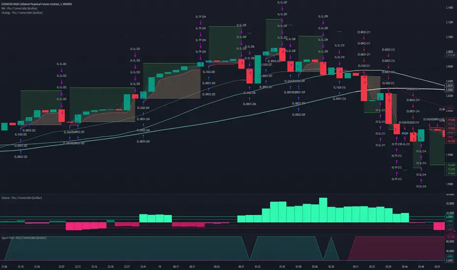
Strategy - Plus / Connectable [Azullian]Discover the advanced capabilities of Strategy Plus, an essential component of the connectable indicator system designed for fast-paced strategy testing, visualization, and building within TradingView. This enhanced version of our foundational connectable strategy indicator seamlessly integrates with all connectable indicators . By utilizing the TradingView input source as a signal connector , it facilitates the linking of indicators to form a cohesive strategy. Each connectable indicator within the system sends signal weight to the next node, culminating in a comprehensive strategy that incorporates advanced customization options, sophisticated signal interpretation, and elaborate backtest labeling. Strategy Plus stands out by offering improved position management and extensive alert messaging capabilities, ensuring effective strategy refinement and backend integration.
█ DISTINCTIVE FEATURES
The Connectable Strategy Plus enhances risk mitigation within the connectable system through its advanced features and capabilities:
• Refined Signal Input Management: Tailor and precisely connect up to two signal filters with enhanced input flexibility, gain control, and strategic direction settings.
• Strategic Position Investment Control: Optimize positioning with versatile investment bases, custom investment percentages, and direction-specific investments for effective risk management.
• Advanced Exit Stop Loss Configuration: Implement custom stop loss tactics with diverse base modes and trailing options for tailored risk management.
• Strategic Exit Take Profit Settings: Apply precision-driven take profit strategies with various calculation modes and dynamic trailing functionality.
• Calibrated Entry Position Allocation: Optimize investment distribution for entry positions, including DCA and BRO trades, for strategic market response.
• Refined Order Setting Customization: Ensure exchange compliance with adjustable order settings, enhancing backtest accuracy and strategy reliability.
• Comprehensive Condition Settings: Define precise conditions for strategy execution, including date range filtering and order/loss limitations.
• Intuitive Visualization: Enhance strategy clarity with customizable visual elements and trade visualization features.
• Advanced Alert Configurations: Stay informed with comprehensive and customizable alerts for effective backend integration.
• Backend Integration With JSON Format: Leverage elaborate and structured data in JSON format for advanced analytics, enhancing decision-making and strategy optimization outside TradingView.
Let's review the separate parts of this indicator.
█ STRATEGY INPUTS
We've provided 2 inputs for connecting a signal filter or indicators or chains (1→, 2→) which are all set to 'Close' by default.
An input has several controls:
• Enable disable: Toggle the entire input on or off
• Input: Connect indicators or signal filter here, choose indicators with a compatible : Signal connector.
• G - Gain: Increase or reduce the strength of the incoming signal by a factor.
• SM - Signal Mode: Choose a trading direction compatible with the settings in your signal filter
• XM - Exit Mode: Determine when to allow to exit your open trade
○ Always: Doesn't take the restrictions into account, this ignores all the settings chosen in ML or MP
○ Restricted: Use both ML and MP conditions
○ Loss: Use the ML condition only, for example: Position will be exited and the exit signal will be allowed only when the loss exceeds the ML parameter
○ Profit: Use the MP condition only for example: Exits will only be allowed when the profit of the position exceeds the condition of the MP parameter
█ POSITION INVESTMENT
Determine the percentage of your trading budget you would like to use in each position based on the strategy's profit or loss.
• LINVB - Loss Investment Base: Choose which base to use to determine the investment percentage when the strategy is in a loss.
○ Equity: Use the equity as the base for percentage calculation.
○ Initial capital: Use the initial capital as the base for percentage calculation.
• LINV% - Loss Investment Percentage: Set a percentage of the chosen investment base as the investment for a new position.
○ For example, when 10% in loss, and a initial capital of $100, and the investment base is set to equity with a percentage of 50%, your investment will be 50% of $90, $45.
• PINVB - Profit Investment Base: Choose which base to use to determine the investment percentage when the strategy is in profit.
○ Equity: Use the equity as the base for percentage calculation.
○ Initial capital: Use the initial capital as the base for percentage calculation.
• PINV% - Profit Investment Percentage: Set a percentage of the chosen investment base as the investment for a new position.
○ For example, when 10% in profit, and an initial capital of $100, and the investment base is set to equity with a percentage of 100%, your investment will be 100% of $110, $110.
• XINVB - Custom Profit Investment Base: Choose which base to use to determine the investment percentage when the strategy is above a custom profit threshold (XT).
○ Equity: Use the equity as the base for percentage calculation.
○ Initial capital: Use the initial capital as the base for percentage calculation.
• XINV% - Custom Profit Investment Percentage: Set a percentage of the chosen investment base as the investment for a new position.
○ For example, when 100% in profit, exceeding the XT threshold of 50%, and an initial capital of $100, and the investment base is set to equity with a percentage of 50%, your investment will be 50% of $200, $100.
• XT% - Custom Profit Threshold: Determine how much profit triggers these custom profit investment settings.
• ELIB% - Entry Long Investment Base: Following previous settings, you can further restrict the investment according to the long trading direction.
○ For instance, if the previous calculation resulted in $45 to be used as an investment, and you've set the ELIB% to 50%, your long position will use 50% of $45, which is $22.5.
• ESIB% - Entry Short Investment Base: Following previous settings, you can further restrict the investment according to the short trading direction.
○ For example, if the previous calculation resulted in $45 to be used as an investment, and you've set the ESIB% to 50%, your short position will use 50% of $45, which is $22.5.
• RISK% - Risk Percentage:
○ Determine how much of the calculated position investment is at risk when the stop-loss is hit.
- For example, 1% of $45 represents a maximum loss of $0.45.
○ Risk percentage works together with the stop loss and the max leverage.
• MXLVG - Maximum Leverage:
○ Investigate the trading rules for your trading pair and use the maximum allowed amount of leverage.
○ To determine the number of contracts to be bought or sold, considering the stop loss and the specified risk percentage, the maximum leverage available will constrain the amount of leverage utilized to ensure that the maximum risk threshold is not exceeded. For instance, suppose the stop loss is set at 1%, and the risk percentage is defined as 10%. Initially, the calculated leverage to be used would be 10. However, if there is a maximum leverage cap set at 5, it would constrain the calculated leverage of 10 to adhere to the maximum limit of 5.
█ EXIT STOP LOSS
Determine the Stop Loss price based on your selected configuration.
As the stop loss is an integral part of the ordered contracts calculation used in conjunction with the Risk and Max leverage, you'll always need to provide a stop loss price.
• SLLB - Stop Loss Long Base: Choose a stop loss mode for calculating stop loss prices in long positions.
○ Risk: Determines the price using the Risk parameter (RISK%) and maximum leverage (MXLVG). In this case, SLLB% will not have any impact.
○ Price Entry + Offset: Calculates the stop loss price based on a offset percentage (SLLB%) from the entry price of the position.
○ Source: Computes the stop loss price based on an external indicator defined in SLLSRC.
- If this results in an invalid price, the calculation will revert to using the price entry + offset.
○ Source + Offset: Determines the stop loss price based on a positive or negative offset percentage (SLLB%) from an external indicator defined in SLLSRC.
- If this results in an invalid price, the calculation will fall back to using the price entry + offset.
• SLLB% - Stop Loss Long Base Percentage: Define an offset percentage that will be applied in the price entry + offset and source + offset stop loss modes.
• SLLSRC - Stop Loss Long Source: Connect an external indicator as the source for stop loss (only those providing price values eg: bollinger bands, moving averages...).
• SLLT - Stop Loss Long Trailing:
○ Fixed: The initial stop loss will be kept and no trailing stop loss will be applied.
○ Trail Stop: Takes into account all settings defined in SLLB and SLLB% and recalculates them with each candle.
- If a better stop loss is computed, it replaces the existing stop loss. In this mode SLLT% will be disregarded.
○ Trail Stop till BE: Similar to trailing stop mode, but it stops trailing when the stop loss reaches the break-even point.
○ Trail Stop from BE: Similar to trailing stop mode, but it starts trailing when the stop loss reaches the break-even point.
○ Trail Price: Computes the trailing stop loss price based on an offset percentage (SLLT%) from the closing price of the current candle.
- If a better stop loss price is calculated, it will be set as the new stop loss price.
○ Trail Price till BE: Similar to the Trail Price mode, but it stops trailing when the stop loss reaches the break-even point.
○ Trail Price from BE: Similar to Trail Price mode, but it starts trailing when the stop loss reaches the break-even point.
○ Trail Incr: Adapts the trailing stop loss price based on the offset percentage (SLLT%).
- Each price change in favor of your position will incrementally adapt the trailing stop loss with SLLT%.
○ Trail Incr till BE: Similar to the Trail Incr mode, but it stops trailing when the stop loss reaches the break-even point.
• SLLT% - Stop Loss Long Trailing Percentage: This percentage serves as an offset or increment depending on your chosen trailing mode.
• SLSB - Stop Loss Short Base: Functions similarly to SLLB but for short positions.
• SLSB% - Stop Loss Short Base Percentage: Functions similarly to SLLB% but for short positions.
• SLSSRC - Stop Loss Short Source: Functions similarly to SLLSRC but for short positions.
• SLST - Stop Loss Short Trailing: Functions similarly to SLLT but for short positions.
• SLST% - Stop Loss Short Trailing Percentage: Functions similarly to SLLT% but for short positions.
█ EXIT TAKE PROFIT
Determine the Take Profit price based on your selected configuration.
• TPLB - Take Profit Long Base: Choose a take profit mode for calculating take profit prices in long positions.
○ Reward: Determines the take profit price using the Risk parameter (RISK%) and the calculated Stop Loss price and the set reward percentage (TPLB%).
- For example: Risk 1%, Calculated Stop loss price: $90, Entry price: $100, Reward (TPLB%): 2%, will result in a take profit price on $120.
○ Price Entry + Offset: Calculates the take profit price based on a offset percentage (TPLB%) from the entry price of the position.
- For example: Entry price: $100, Offset (TPLB%): 2%, will result in a take profit price on $102.
○ Source: Computes the take profit price based on an external input from another indicator defined in TPLSRC.
- If this results in an invalid price, the calculation will revert to using the price entry + offset.
○ Source + Offset: Determines the take profit price based on a positive or negative offset percentage (TPLB%) from an external indicator inpuy defined in TPLSRC.
- If this results in an invalid price, the calculation will fall back to using the price entry + offset.
• TPLB% - Take Profit Long Base Percentage: Define an offset percentage that will be applied in the price entry + offset and source + offset take profit modes.
• TPLSRC - Take Profit Long Source: Choose to connect an external indicator as the source for take profit (of course only those which provide price values eg: bollinger bands, moving averages... but not oscillators).
• TPLT - Take Profit Long Trailing:
○ Fixed: The initial take profit will be kept and no trailing take profit will be applied.
○ Trail Profit: Takes into account all settings defined in TPLB and TPLB% and recalculates them with each candle.
- If an applicable take profit is computed, it replaces the existing take profit. In this mode TPLT% will be disregarded.
○ Trail Profit till BE: Similar to trailing profit mode, but it stops trailing when the take profit reaches the break-even point.
○ Trail Profit from BE: Similar to trailing profit mode, but it starts trailing when the take profit reaches the break-even point.
○ Trail Price: Computes the trailing take profit price based on an offset percentage (TPLT%) from the closing price of the current candle.
- If an applicable take profit price is calculated, it will be set as the new take profit price.
○ Trail Price till BE: Similar to the Trail Price mode, but it stops trailing when the take profit reaches the break-even point.
○ Trail Price from BE: Similar to Trail Price mode, but it starts trailing when the take profit reaches the break-even point.
○ Trail Incr: Adapts the trailing take profit price based on the offset percentage (TPLT%). Each price change against your position will incrementally adapt the trailing take profit with TPLT%.
○ Trail Incr till BE: Similar to the Trail Incr mode, but it stops trailing when the take profit reaches the break-even point.
• TPLT% - Take Profit Long Trailing Percentage: This percentage serves as an offset or increment depending on your chosen trailing mode.
• TPSB - Take Profit Short Base: Functions similarly to TPLB but for short positions.
• TPSB% - Take Profit Short Base Percentage: Functions similarly to TPLB% but for short positions.
• TPSSRC - Take Profit Short Source: Functions similarly to TPLSRC but for short positions.
• TPST - Take Profit Short Trailing: Functions similarly to TPLT but for short positions.
• TPST% - Take Profit Short Trailing Percentage: Functions similarly to TPLT% but for short positions.
█ ENTRY INVESTMENT DISTRIBUTION
Based on your position investment calculation you can distribute the position investment accross the initial opening trade of the position (SIG%) or the follow up Dollar Cost Averaging (DCA%) or Break Out (BRO%) trades.
For example: SIG%: 10%, DCA%: 45%, BRO%: 45% and the calculated Position Investment is $100, then the initial trade will receive $10, DCA will receive $45, and BRO will receive $45 to work with. Disable BRO and or DCA by setting them to 0%. Keep in mind that the sum of SIG, BRO and DCA may not exceed 100%.
• SIG% - Initial order investment percentage based on the signal: The percentage of the position investment distributed over normal trades.
• DCA% - Dollar Cost Averaging investment percentage: The percentage of the position investment distributed to DCA trades.
• BRO% - Break Out investment percentage: The percentage of the position investment distributed to BRO trades.
█ ENTRY DCA
DCA (Dollar-Cost Averaging) is a risk mitigation strategy where the allocated DCA% budget from the Entry Investment Distribution is distributed among x levels (DCA#) based on calculated prices (DPLM) and order sizes (DOSM), when prices move against your position.
• DCA# - Maximum DCA levels: Set the maximum number of DCA levels.
• DPLM - DCA Price Level Mode: Choose a price level mode that determines at which prices the additional purchases are distributed:
○ Linear: Entry prices are evenly spaced at regular intervals.
○ QuadIn: Entry prices are front-loaded, with more at the beginning and fewer later.
○ QuadOut: Entry prices are back-loaded, with fewer at the beginning and more later.
○ QuadInOut: Entry prices start front-loaded, then become back-loaded.
○ CubicIn: Similar to QuadIn but with a smoother front-loaded distribution.
○ CubicOut: Similar to QuadOut but with a smoother back-loaded distribution.
○ ExpoIn: Entry prices are exponentially increasing, starting small and growing.
○ ExpoOut: Entry prices are exponentially decreasing, starting large and reducing.
○ ExpoInOut: Entry prices start exponentially increasing, then decrease exponentially.
• DOSM - DCA Order Size Mode: Choose a DCA budget distribution mode for order sizes:
○ Linear: Order sizes are evenly spaced at regular intervals.
○ QuadIn: Order sizes are front-loaded, with larger orders at the beginning and smaller ones later.
○ QuadOut: Order sizes are back-loaded, with smaller orders at the beginning and larger ones later.
○ QuadInOut: Order sizes start front-loaded and transition to back-loaded.
○ CubicIn: Similar to QuadIn but with a smoother front-loaded distribution of order sizes.
○ CubicOut: Similar to QuadOut but with a smoother back-loaded distribution of order sizes.
○ ExpoIn: Order sizes exponentially increase, starting small and growing.
○ ExpoOut: Order sizes exponentially decrease, starting large and reducing.
○ ExpoInOut: Order sizes start exponentially increasing, then decrease exponentially.
For a visual representation of the price or order size distribution modes, refer to online easing curves.
█ ENTRY BRO
BRO (Break Out) is a risk mitigation strategy where the allocated BRO% budget from the Entry Investment Distribution is distributed among x levels (BRO#) based on calculated prices (BPLM) and order sizes (BOSM), when prices move in favor of your position.
• BRO# - Maximum BRO levels: Set the maximum number of BRO levels.
• BPLM - BRO Price Level Mode: Choose a price level mode that determines at which prices the additional purchases are distributed:
○ Distribution easing modes work similar as the DCA easing modes.
• BOSM - BRO Order Size Mode: Choose a BRO budget distribution mode for order sizes:
○ Distribution easing modes work similar as the DCA easing modes.
█ ORDER SETTINGS
Fine-tune accuracy to match your exchange's trading constraints, enhancing backtest precision with these settings, default settings are least restrictive for crypto trading pairs.
• MINP - Mininmum Position Notional Value: Exchange-defined minimum notional value for positions:
○ Calculated based on your exchange's rules and is the minimum total value your position must hold to meet their requirements It is calculated by multiplying Quantity with price and leverage.
○ It helps ensure your trades align with your exchange's standards.
• MAXP - Maximum Position Notional Value: Exchange-defined maximum notional value for positions:
○ Similar to MINP, this value is calculated based on your exchange's rules and represents the maximum total value allowed for your position.
• MINQ - Mininmum Order Quantity: Least permissible order quantity based on exchange rules:
○ This is the smallest quantity of an asset that your exchange allows you to trade in a single order.
• MAXQ - Maximum Order Quantity: Highest permissible order quantity according to exchange rules:
○ Opposite of MINQ, this is the largest quantity of an asset you can trade in a single order as defined by your exchange.
• DECP - Decimals in Order Price: Allowed decimal places in order prices as per exchange specifications:
○ This value specifies the number of decimal places you can use when specifying the price of an order.
• DECQ - Decimals in Order Quantity: Permitted decimal places in order quantities according to exchange specifications:
○ Similar to DECP, this value indicates the number of decimal places you can use when specifying the quantity of an asset in an order.
█ STRATEGY CONDITIONS
Specify when the strategy is permitted to execute trades.
• DATE: Enable the Date Range filter to restrict entries to a specific date range.
○ START: Set a start date and hour to commence trading.
○ END: Set an end date and hour to conclude trading within the defined range.
• IDO - Maximum Intraday Orders: Limit the number of orders the strategy can place within a single trading day. Upon reaching this limit, the strategy temporarily halts further entries for the day.
• DL% - Maximum Intraday Loss%: Set a threshold for the maximum allowable intraday loss as a percentage of equity. When exceeded, the strategy temporarily suspends trading for the day.
• CLD - Maximum Consecutive Loss Days: Define the maximum number of consecutive days the strategy can incur losses. Upon reaching this limit, the strategy halts trading and avoids new entries.
• DD% - Maximum Drawdown: Specify the maximum permissible drawdown as a percentage of equity. If this limit is met, the strategy halts trading and refrains from placing additional entries.
• TP% - Total Profit %: Establish a target for the total profit percentage the strategy aims to achieve. Once this target is attained, the strategy halts trading and refrains from initiating new entries.
• TL% - Total Loss %: Define a limit for the total loss percentage relative to the initial capital. If this limit is exceeded, the strategy discontinues trading and refrains from placing further entries.
■ VISUALS
• LINE: Activate a colored dashed diagonal line to visually connect the entry and exit points of positions.
• SLTP: Enable visualization of stop loss, take profit, and break-even levels.
• PNL: Enable Break-Even and Close Lines along with a colored area in between to visualize profit and loss.
• ☼: Brightness % : Adjust the opacity of the plotted trading visuals.
• P - Profit Color : Choose the color for profit-related elements.
• L - Loss Color: Choose the color for loss-related elements.
• B - Breakeven Color : Select the color for break-even points.
• EL - Long Color: Specify the color for long positions.
• ES - Short Color: Specify the color for short positions.
• TRADE LABELING: For better analysis we've labeled all entries and exits conform with the type of order your strategy has executed, some examples:
○ EL-SIG0-124: Enter Long - Signal 0 - Position 124
○ EL-BRO1-130: Enter Long - BRO1 - Position 130
○ EL-BRO2-130: Enter Long - BRO2 - Position 130
○ ES-DCA1-140: Enter Short - DCA1 - Position 140
○ XS-DCA2-140: Exit Short - DCA2 - Position 140
○ XL-TP-150: Exit Long - Take Profit - Position 150
○ XS-TP-154: Exit Short - Take Profit - Position 154
○ XL-SL-160: Exit Long - Stop Loss - Position 160
○ XS-SL-164: Exit Short - Stop Loss - Position 164
○ XS-CND-165: Exit Short - Strategy Condition - Max intraday loss - Position 165
■ ALERT SETTINGS
For developers and those who wish to integrate TradingView alerts into their backend systems, we offer comprehensive labeling options.
• ALID: A unique identifier you've assigned to your alert.
• NAME: A structured name you've given to this strategy.
• LAYOUT: The layout key of the strategy, allowing direct chart linking from your backend.
• SYMBOL: The symbol on which the strategy operates.
○ ONCE: You can choose to include this information only in the first message to reduce message size and repetition in follow-up messages. (max. 4096 characters)
• TICK: The ticker for the strategy.
• CHART: The chart parameter containing the timeframe.period and timeframe.multiplier.
○ ONCE: You can choose to include this information only in the first message to reduce message size and repetition in follow-up messages. (max. 4096 characters)
• BAR: Includes bar information in the alert message.
• STRATEGY: Adds strategy inputs to the alert message.
○ ONCE: You can choose to include this information only in the first message to reduce message size and repetition in follow-up messages. (max. 4096 characters)
• PERFORMANCE: Incorporates strategy performance data into the alert message.
• SIGNAL: Appends received signal weights (EL, XL, ES, XS) to the alert message.
• ORDERS: Includes order details in the alert message.
• TAGS: Adds up to 6 tags and their corresponding values to the alert message.
○ ONCE: You can choose to include this information only in the first message to reduce message size and repetition in follow-up messages. (max. 4096 characters)
Of course we can't neglect letting you in on how this juicy JSON would look (without the // comments):
{
"id": 20726, // Message Id
"t": "2023-11-01T10:35:00Z", // Message Time
"al": { // Alert
"id": "639bfa9a-5f01-4031-8880-7ec01e972055", // Alert Id
"n": "TEST04", // Name
"l": "ABC123" // Layout
},
"sym": { // Symbol
"typ": "crypto", // Type
"r": "DOGEUSD.PM", // Root
"pre": "KRAKEN", // Prefix
"tc": "DOGEUSD.PM", // Ticker
"bc": "DOGE", // BaseCurrency
"c": "USD", // Currency
"d": "DOGEUSD Multi Collateral Perpetual Futures Contract", // Description
"mtc": 0.000001, // MinTick
"pv": 1, // PointValue
"ct": "PF_DOGEUSD" // CustomTicker
},
"ch": { // Chart
"pd": "1", // Period
"mul": 1 // Multiplier
},
"bar": { // Bar
"id": 20725, // Index
"t": "2023-11-01T10:33:00Z", // Time
"o": 0.066799, // Open
"h": 0.066799, // High
"l": 0.066799, // Low
"c": 0.066799, // Close
"v": 2924 // Vol
},
"strat": { // Strategy
"n": "Strategy - Plus / Connectable ", // Name
"sig": { // Signal
"c1e": true, // Connector1Enabled
"c1s": 500500.500501, // Connector1Source
"c1g": 1, // Connector1Gain
"c2e": false, // Connector2Enabled
"c2s": 0.067043, // Connector2Source
"c2g": 1, // Connector2Gain
"sm": "Swing (EL, ES)", // SignalMode
"xm": "Always", // ExitMode
"mlp": 0.01, // ExitModeMinPercLoss
"mpp": 0.01 // ExitModeMinPercProfit
},
"inv": { // Investment
"lb": "Equity", // LossBase
"lp": 50, // LossPerc
"pb": "Equity", // ProfitBase
"pp": 100, // ProfitPerc
"pcb": "Equity", // ProfitCustomBase
"pcp": 100, // ProfitCustomPerc
"pct": 10000, // ProfitCustomThreshold
"elp": 100, // LongPerc
"esp": 100, // ShortPerc
"rsk": 1, // MaxRisk
"lvg": 10 // MaxLeverage
},
"sl": { // StopLoss
"lb": "Price Entry + Offset", // LongBase
"lp": 0.2, // LongPerc
"lsrc": 0.067043, // LongSource
"lt": "Trail Stop", // LongTrailMode
"ltp": 0.2, // LongTrailPerc
"sb": "Price Entry + Offset", // ShortBase
"sp": 0.2, // ShortPerc
"ssrc": 0.067043, // ShortSource
"st": "Trail Stop", // ShortTrailMode
"stp": 0.2 // ShortTrailPerc
},
"tp": { // TakeProfit
"lb": "Price Entry + Offset", // LongBase
"lp": 1, // LongPerc
"lsrc": 0.067043, // LongSource
"lt": "Fixed", // LongTrailMode
"ltp": 1, // LongTrailPerc
"sb": "Price Entry + Offset", // ShortBase
"sp": 1, // ShortPerc
"ssrc": 0.067043, // ShortSource
"st": "Fixed", // ShortTrailMode
"stp": 1 // ShortTrailPerc
},
"dis": { // Distribution
"sigp": 10, // SignalPerc
"dcap": 0, // DCAPerc
"brop": 90 // BROPerc
},
"dca": { // DCA
"lvl": 3, // Levels
"pl": "linear", // ModePriceLevel
"os": "linear" // ModeOrderSize
},
"bro": { // BRO
"lvl": 3, // Levels
"pl": "expoIn", // ModePriceLevel
"os": "cubicOut" // ModeOrderSize
},
"ord": { // OrderSettings
"pmin": 5, // PNVMin
"pmax": 30000000, // PNVMax
"qmin": 0, // QtyMin
"qmax": 1000000000, // QtyMax
"dp": 6, // DecPrice
"dq": 6 // DecQty
},
"cnd": { // Conditions
"de": true, // DateRangeEnabled
"start": "2023-11-01T10:30:00Z", // StartTime
"end": "2024-12-31T23:30:00Z", // EndTime
"idoe": false, // MaxIntradayOrdersEnabled
"ido": 100, // MaxIntradayOrders
"dle": false, // MaxIntradayLossEnabled
"dl": 10, // MaxIntradayLossPerc
"clde": false, // MaxConsLossDaysEnabled
"cld": false, // MaxConsLossDays
"dde": false, // MaxDrawdownEnabled
"dd": 100, // MaxDrawdownPerc
"mpe": false, // MaxProfitEnabled
"mp": 200, // MaxProfitPerc
"mle": false, // MaxLossEnabled
"ml": -50 // MaxLossPerc
}
},
"perf": { // Performance
"ic": 1000, // InitialCapital
"eq": 1000, // Equity
"np": 0, // NetProfit
"op": 0, // OpenProfit
"ct": 0, // ClosedTrades
"ot": 0, // OpenTrades
"p": "FLAT", // MarketPosition
"ps": 0, // MarketPositionSize
"pp": "FLAT", // PreviousMarketPosition
"pps": 0 // PreviousMarketPositionSize
},
"sig": { // Signal
"el": 0, // EL
"xl": 0, // XL
"es": 6, // ES
"xs": 0 // XS
},
"ord": ,
"tag":
}
█ USAGE OF CONNECTABLE INDICATORS
■ Connectable chaining mechanism
Connectable indicators can be connected directly to the signal monitor, signal filter or strategy , or they can be daisy chained to each other while the last indicator in the chain connects to the signal monitor, signal filter or strategy. When using a signal filter you can chain the filter to the strategy input to make your chain complete.
• Direct chaining: Connect an indicator directly to the signal monitor, signal filter or strategy through the provided inputs (→).
• Daisy chaining: Connect indicators using the indicator input (→). The first in a daisy chain should have a flow (⌥) set to 'Indicator only'. Subsequent indicators use 'Both' to pass the previous weight. The final indicator connects to the signal monitor, signal filter, or strategy.
■ Set up this indicator with signals and a signal filter
The indicator provides visual cues based on signal conditions. However, its weight system is best utilized when paired with a connectable signal filter, monitor, or strategy .
Let's connect the Strategy - Plus to a connectable signal filter and connectable indicators :
1. Load all relevant indicators
• Load MA - Plus / Connectable
• Load Signal filter - Plus / Connectable
• Load Strategy - Plus / Connectable
2. Signal Filter Plus: Connect the MA - Plus to the Signal Filter
• Open the signal filter settings
• Choose one of the five input dropdowns (1→, 2→, 3→, 4→, 5→) and choose : MA - Plus / Connectable: Signal Connector
• Toggle the enable box before the connected input to enable the incoming signal
3. Signal Filter: Update the filter settings if needed
• The default filter mode for the trading direction is SWING, and is compatible with the default settings in the strategy and indicators.
4. Signal Filter: Update the weight threshold settings if needed
• All connectable indicators load by default with a score of 6 for each direction (EL, XL, ES, XS)
• By default, weight threshold is 'ABOVE' Threshold 1 (TH1) and Threshold 2 (TH2), both set at 5. This allows each occurrence to score, as the default score is 1 point above the threshold.
5. Strategy Plus: Connect one of the strategy plus inputs to the signal filters signal connector in the strategy settings
• Select a strategy input → and select the Signal filter - Plus: Signal connector
6. Strateg Plus: Enable filter compatible directions
• As the default setting of the filter is SWING, we should also set the SM (Strategy mode) to SWING.
7. Strateg Plus: You're ready to start optimizing
• Dive into all parameters and start optimizing your backtesting results.
█ BENEFITS
• Adaptable Modular Design: Arrange indicators in diverse structures via direct or daisy chaining, allowing tailored configurations to align with your analysis approach.
• Streamlined Backtesting: Simplify the iterative process of testing and adjusting combinations, facilitating a smoother exploration of potential setups.
• Intuitive Interface: Navigate TradingView with added ease. Integrate desired indicators, adjust settings, and establish alerts without delving into complex code.
• Signal Weight Precision: Leverage granular weight allocation among signals, offering a deeper layer of customization in strategy formulation.
• Advanced Signal Filtering: Define entry and exit conditions with more clarity, granting an added layer of strategy precision.
• Clear Visual Feedback: Distinct visual signals and cues enhance the readability of charts, promoting informed decision-making.
• Standardized Defaults: Indicators are equipped with universally recognized preset settings, ensuring consistency in initial setups across different types like momentum or volatility.
• Reliability: Our indicators are meticulously developed to prevent repainting. We strictly adhere to TradingView's coding conventions, ensuring our code is both performant and clean.
█ COMPATIBLE INDICATORS
Each indicator that incorporates our open-source 'azLibConnector' library and adheres to our conventions can be effortlessly integrated and used as detailed above.
For clarity and recognition within the TradingView platform, we append the suffix ' / Connectable' to every compatible indicator.
█ COMMON MISTAKES, CLARIFICATIONS AND TIPS
• Removing an indicator from a chain: Deleting a linked indicator and confirming the "remove study tree" alert will also remove all underlying indicators in the object tree. Before removing one, disconnect the adjacent indicators and move it to the object stack's bottom.
• Point systems: The azLibConnector provides 500 points for each direction (EL: Enter long, XL: Exit long, ES: Enter short, XS: Exit short) Remember this cap when devising a point structure.
• Flow misconfiguration: In daisy chains the first indicator should always have a flow (⌥) setting of 'indicator only' while other indicator should have a flow (⌥) setting of 'both'.
• Hide attributes: As connectable indicators send through quite some information you'll notice all the arguments are taking up some screenwidth and cause some visual clutter. You can disable arguments in Chart Settings / Status line.
• Layout and abbreviations: To maintain a consistent structure, we use abbreviations for each input. While this may initially seem complex, you'll quickly become familiar with them. Each abbreviation is also explained in the inline tooltips.
• Inputs: Connecting a connectable indicator directly to the strategy delivers the raw signal without a weight threshold, meaning every signal will trigger a trade.
• Layout and Abbreviations: Abbreviations streamline structure and input identification. Although they may seem complex initially, inline tooltips provide explanations, facilitating quick acclimatization.
• Total Trade Limit Error & Date-Time Filter: For deep backtesting, be mindful of the total trade limit. Utilize the date-time filter to narrow the test scope and avoid TradingView order limits.
• Calculation Timeout: Encounter a timeout? Adjust any parameter slightly to restart the calculation process.
• Message Character Limit: To stay within message character limits, consider turning off certain features or setting some to 'once'.
• Direct Indicator-to-Strategy Connection: When connecting an indicator directly to a strategy without thresholds, the strategy will default to long if weights are equally assigned.
• Pyramid Enabling with DCA and BRO: Activate pyramid orders, enabling you to optimize your strategy during Dollar Cost Averaging and Break Out trades.
• Recalculate & Fill Orders Properties: Adjusting these default settings in strategy properties tab may lead to unexpected behavior when backtesting. Approach with caution.
• Optimized for Crypto: Our indicators have been optimized and tested primarily on cryptocurrency markets. Results in other markets may vary.
• Inline Tooltips Documentation: Detailed documentation and guidance are available via inline tooltips for immediate assistance.
• Strategy Settings Margin: Set margin to 1 to be able to apply leverage.
• Styling Panel: Explore the styling panel to disable labels or any other visual cues to reduce clutter on busy charts, enhancing visual clarity and personalization.
• Applying Leverage on Spot Markets: Ensure that maximum leverage on spot markets is configured to 1.
• Unrealistic Order Sizes: Verify that the order book can accommodate your backtested order sizes.
█ A NOTE OF GRATITUDE
Through years of exploring TradingView and Pine Script, we've drawn immense inspiration from the community's knowledge and innovation. Thank you for being a constant source of motivation and insight.
█ RISK DISCLAIMER
Azullian's content, tools, scripts, articles, and educational offerings are presented purely for educational and informational uses. Please be aware that past performance should not be considered a predictor of future results.
Long-Only Opening Range Breakout (ORB) with Pivot PointsIntraday Trading Strategy: Long-Only Opening Range Breakout (ORB) with Pivot Points
Background:
Opening Range Breakout (ORB) is a popular long-only trading strategy that capitalizes on the early morning volatility in financial markets. It's based on the idea that the initial price movements during the first few minutes or hours of the trading day can set the tone for the rest of the session. The strategy involves identifying a price range within which the asset trades during the opening period and then taking long positions when the price breaks out to the upside of this range.
Pivot Points are a widely used technical indicator in trading. They represent potential support and resistance levels based on the previous day's price action. Pivot points are calculated using the previous day's high, low, and close prices and can help traders identify key price levels for making trading decisions.
How to Use the Script:
Initialization: This script is written in Pine Script, a domain-specific language for trading strategies on the TradingView platform. To use this script, you need to have access to TradingView.
Apply the Script: You can do this by adding it to your favorites, then selecting the script in the indicators list under favorites or by searching for it by name under community scripts.
Customize Settings: The script allows you to customize various settings through the TradingView interface. These settings include:
Opening Session: You can set the time frame for the opening session.
Max Trades per Day: Specify the maximum number of long trades allowed per trading day.
Initial Stop Loss Type: Choose between using a percentage-based stop loss or the previous candles low for stop loss calculations.
Stop Loss Percentage: If you select the percentage-based stop loss, specify the percentage of the entry price for the stop loss.
Backtesting Start and End Time: Set the time frame for backtesting the strategy.
Strategy Signals:
The script will display pivot points in blue (R1, R2, R3, R4, R5) and half-pivot points in gray (R0.5, R1.5, R2.5, R3.5, R4.5) on your chart.
The green line represents the opening range.
The script generates long (buy) signals based on specific conditions:
---The open price is below the opening range high (h).
---The current high price is above the opening range high.
---Pivot point R1 is above the opening range high.
---It's a long-only strategy designed to capture upside breakouts.
---It also respects the maximum number of long trades per day.
The script manages long positions, calculates stop losses, and adjusts long positions according to the defined rules.
Trailing Stop Mechanism
The script incorporates a dynamic trailing stop mechanism designed to protect and maximize profits for long positions. Here's how it works:
1. Initialization:
The script allows you to choose between two types of initial stop loss:
---Percentage-based: This option sets the initial stop loss as a percentage of the entry price.
---Previous day's low: This option sets the initial stop loss at the previous day's low.
2. Setting the Initial Stop Loss (`sl_long0`):
The initial stop loss (`sl_long0`) is calculated based on the chosen method:
---If "Percentage" is selected, it calculates the stop loss as a percentage of the entry price.
---If "Previous Low" is selected, it sets the stop loss at the previous day's low.
3. Dynamic Trailing Stop (`trail_long`):
The script then monitors price movements and uses a dynamic trailing stop mechanism (`trail_long`) to adjust the stop loss level for long positions.
If the current high price rises above certain pivot point levels, the trailing stop is adjusted upwards to lock in profits.
The trailing stop levels are calculated based on pivot points (`r1`, `r2`, `r3`, etc.) and half-pivot points (`r0.5`, `r1.5`, `r2.5`, etc.).
The script checks if the high price surpasses these levels and, if so, updates the trailing stop accordingly.
This dynamic trailing stop allows traders to secure profits while giving the position room to potentially capture additional gains.
4. Final Stop Loss (`sl_long`):
The script calculates the final stop loss level (`sl_long`) based on the following logic:
---If no position is open (`pos == 0`), the stop loss is set to zero, indicating there is no active stop loss.
---If a position is open (`pos == 1`), the script calculates the maximum of the initial stop loss (`sl_long0`) and the dynamic trailing stop (`trail_long`).
---This ensures that the stop loss is always set to the more conservative of the two values to protect profits.
5. Plotting the Stop Loss:
The script plots the stop loss level on the chart using the `plot` function.
It will only display the stop loss level if there is an open position (`pos == 1`) and it's not a new trading day (`not newday`).
The stop loss level is shown in red on the chart.
By combining an initial stop loss with a dynamic trailing stop based on pivot points and half-pivot points, the script aims to provide a comprehensive risk management mechanism for long positions. This allows traders to lock in profits as the price moves in their favor while maintaining a safeguard against adverse price movements.
End of Day (EOD) Exit:
The script includes an "End of Day" (EOD) exit mechanism to automatically close any open positions at the end of the trading day. This feature is designed to manage and control positions when the trading day comes to a close. Here's how it works:
1. Initialization:
At the beginning of each trading day, the script identifies a new trading day using the `is_newbar('D')` condition.
When a new trading day begins, the `newday` variable becomes `true`, indicating the start of a new trading session.
2. Plotting the "End of Day" Signal:
The script includes a plot on the chart to visually represent the "End of Day" signal. This is done using the `plot` function.
The plot is labeled "DayEnd" and is displayed as a comment on the chart. It signifies the EOD point.
3. EOD Exit Condition:
When the script detects that a new trading day has started (`newday == true`), it triggers the EOD exit condition.
At this point, the script proceeds to close all open positions that may have been active during the trading day.
4. Closing Open Positions:
The `strategy.close_all` function is used to close all open positions when the EOD exit condition is met.
This function ensures that any remaining long positions are exited, regardless of their current profit or loss.
The function also includes an `alert_message`, which can be customized to send an alert or notification when positions are closed at EOD.
Purpose of EOD Exit
The "End of Day" exit mechanism serves several essential purposes in the trading strategy:
Risk Management: It helps manage risk by ensuring that positions are not left open overnight when markets can experience increased volatility.
Capital Preservation: Closing positions at EOD can help preserve trading capital by avoiding potential adverse overnight price movements.
Rule-Based Exit: The EOD exit is rule-based and automatic, ensuring that it is consistently applied without emotions or manual intervention.
Scalability: It allows the strategy to be applied to various markets and timeframes where EOD exits may be appropriate.
By incorporating an EOD exit mechanism, the script provides a comprehensive approach to managing positions, taking profits, and minimizing risk as each trading day concludes. This can be especially important in volatile markets like cryptocurrencies, where overnight price swings can be significant.
Backtesting: The script includes a backtesting feature that allows you to test the strategy's performance over historical data. Set the start and end times for backtesting to see how the long-only strategy would have performed in the past.
Trade Execution: If you choose to use this script for live trading, make sure you understand the risks involved. It's essential to set up proper risk management, including position sizing and stop loss orders.
Monitoring: Monitor the long-only strategy's performance over time and be prepared to make adjustments as market conditions change.
Disclaimer: Trading carries a risk of capital loss. This script is provided for educational purposes and as a starting point for your own long-only strategy development. Always do your own research and consider seeking advice from a qualified financial professional before making trading decisions.

Hash Momentum Strategy# Hash Momentum Strategy
## 📊 Overview
The **Hash Momentum Strategy** is a professional-grade momentum trading system designed to capture strong directional price movements with precision timing and intelligent risk management. Unlike traditional EMA crossover strategies, this system uses momentum acceleration as its primary signal, resulting in earlier entries and better risk-to-reward ratios.
---
## ⚡ What Makes This Strategy Unique
### 1. Momentum-Based Entry System
Most strategies rely on lagging indicators like moving average crossovers. This strategy captures momentum *acceleration* - entering when price movement is gaining strength, not after the move has already happened.
### 2. Programmable Risk-to-Reward
Set your exact R:R ratio (1:2, 1:2.5, 1:3, etc.) and the strategy automatically calculates stop loss and take profit levels. No more guessing or manual calculations.
### 3. Smart Partial Profit Taking
Lock in profits at multiple stages:
- **First TP**: Take 50% off at 2R
- **Second TP**: Take 40% off at 2.5R
- **Final TP**: Let 10% ride to maximum target
This approach locks in gains while letting winners run.
### 4. Dynamic Momentum Threshold
Uses ATR (Average True Range) multiplied by your threshold setting to adapt to market volatility. Volatile markets = higher threshold. Quiet markets = lower threshold.
### 5. Trade Cooldown System
Prevents overtrading and revenge trading by enforcing a cooldown period between trades. Configurable from 1-24 bars.
### 6. Optional Session & Weekend Filters
Filter trades by Tokyo, London, and New York sessions. Optional weekend-off toggle to avoid low-liquidity periods.
---
## 🎯 How It Works
### Signal Generation
**STEP 1: Calculate Momentum**
- Momentum = Current Price - Price
- Check if Momentum > ATR × Threshold Multiplier
- Momentum must be accelerating (positive change in momentum)
**STEP 2: Confirm with EMA Trend Filter**
- Long: Price must be above EMA
- Short: Price must be below EMA
**STEP 3: Check Filters**
- Not in cooldown period
- Valid session (if enabled)
- Not weekend (if enabled)
**STEP 4: ENTRY SIGNAL TRIGGERED**
### Risk Management Example
**Example Long Trade:**
- Entry: $100
- Stop Loss: $97.80 (2.2% risk)
- Risk Amount: $2.20
**Take Profit Levels:**
- TP1: $104.40 (2R = $4.40) → Close 50%
- TP2: $105.50 (2.5R = $5.50) → Close 40%
- Final: $105.50 (2.5R) → Close remaining 10%
---
## ⚙️ Settings Guide
### Core Strategy
**Momentum Length** (Default: 13)
Number of bars for momentum calculation. Higher = stronger but fewer signals.
**Momentum Threshold** (Default: 2.25)
ATR multiplier. Higher = only trade biggest moves.
**Use EMA Trend Filter** (Default: ON)
Only long above EMA, short below EMA.
**EMA Length** (Default: 28)
Period for trend-confirming EMA.
### Filters
**Use Trading Session Filter** (Default: OFF)
Restrict trading to specific sessions.
**Tokyo Session** (Default: OFF)
Trade during Asian hours (00:00-09:00 JST).
**London Session** (Default: OFF)
Trade during European hours (08:00-17:00 GMT).
**New York Session** (Default: OFF)
Trade during US hours (08:00-17:00 EST).
**Weekend Off** (Default: OFF)
Disable trading on Saturdays and Sundays.
### Risk Management
**Stop Loss %** (Default: 2.2)
Fixed percentage stop loss from entry.
**Risk:Reward Ratio** (Default: 2.5)
Your target reward as multiple of risk.
**Use Partial Profit Taking** (Default: ON)
Take profits in stages.
**First TP R:R** (Default: 2.0)
First target as multiple of risk.
**First TP Size %** (Default: 50)
Percentage of position to close at TP1.
**Second TP R:R** (Default: 2.5)
Second target as multiple of risk.
**Second TP Size %** (Default: 40)
Percentage of position to close at TP2.
### Trade Management
**Use Trade Cooldown** (Default: ON)
Prevent overtrading.
**Cooldown Bars** (Default: 6)
Bars to wait after closing a trade.
---
## 🎨 Visual Elements
### Chart Indicators
🟢 **Green Dot** (below bar) = Long entry signal
🔴 **Red Dot** (above bar) = Short entry signal
🔵 **Blue X** (above bar) = Long position closed
🟠 **Orange X** (below bar) = Short position closed
**EMA Line** = Trend direction (green when bullish, red when bearish)
**White Line** = Entry price
**Red Line** = Stop loss level
**Green Lines** = Take profit levels (TP1, TP2, Final)
### Dashboard
When not in real-time mode, a dashboard displays:
- Current position (LONG/SHORT/FLAT)
- Entry price
- Stop loss price
- Take profit price
- R:R ratio
- Current momentum strength
- Total trades
- Win rate
- Net profit %
---
## 📈 Recommended Settings by Timeframe
### 1-Hour Timeframe (Default)
- Momentum Length: 13
- Momentum Threshold: 2.25
- EMA Length: 28
- Stop Loss: 2.2%
- R:R Ratio: 2.5
- Cooldown: 6 bars
### 4-Hour Timeframe
- Momentum Length: 24-36
- Momentum Threshold: 2.5
- EMA Length: 50
- Stop Loss: 3-4%
- R:R Ratio: 2.0-2.5
- Cooldown: 6-8 bars
### 15-Minute Timeframe
- Momentum Length: 8-10
- Momentum Threshold: 2.0
- EMA Length: 20
- Stop Loss: 1.5-2%
- R:R Ratio: 2.0
- Cooldown: 4-6 bars
---
## 🔧 Optimization Tips
### Want More Trades?
- Decrease Momentum Threshold (2.0 instead of 2.25)
- Decrease Momentum Length (10 instead of 13)
- Decrease Cooldown Bars (4 instead of 6)
### Want Higher Quality Trades?
- Increase Momentum Threshold (2.5-3.0)
- Increase Momentum Length (18-24)
- Increase Cooldown Bars (8-10)
### Want Lower Drawdown?
- Increase Cooldown Bars
- Use tighter stop loss
- Enable session filters (trade only high-liquidity sessions)
- Enable Weekend Off
### Want Higher Win Rate?
- Increase R:R Ratio (may reduce total profit)
- Increase Momentum Threshold (fewer but stronger signals)
- Use longer EMA for trend confirmation
---
## 📊 Performance Expectations
Based on typical backtesting results:
- **Win Rate**: 35-45%
- **Profit Factor**: 1.5-2.0
- **Risk:Reward**: 1:2.5 (configurable)
- **Max Drawdown**: 10-20%
- **Trades/Month**: 8-15 (1H timeframe)
**Note:** Win rate may appear low, but with 2.5:1 R:R, you only need ~29% win rate to break even. The strategy aims for quality over quantity.
---
## 🎓 Strategy Logic Explained
### Why Momentum > EMA Crossover?
**EMA Crossover Problems:**
- Signals lag behind price
- Late entries = poor R:R
- Many false signals in ranging markets
**Momentum Advantages:**
- Catches moves as they start accelerating
- Earlier entries = better R:R
- Adapts to volatility via ATR
### Why Partial Profit Taking?
**Without Partial TPs:**
- All-or-nothing approach
- Winners often turn to losers
- High stress watching open positions
**With Partial TPs:**
- Lock in 50% at first target
- Reduce risk to breakeven
- Let remainder ride for bigger gains
- Lower psychological pressure
### Why Trade Cooldown?
**Without Cooldown:**
- Revenge trading after losses
- Overtrading in choppy markets
- Emotional decision-making
**With Cooldown:**
- Forces discipline
- Waits for new setup to develop
- Reduces transaction costs
- Better signal quality
---
## ⚠️ Important Notes
1. **This is a momentum strategy, not an EMA strategy**
The EMA only confirms trend direction. Momentum generates the actual signals.
2. **Backtest thoroughly before live trading**
Past performance ≠ future results. Test on your specific asset and timeframe.
3. **Use proper position sizing**
Risk 1-2% of account per trade maximum. The strategy uses 100% equity by default (adjust in Properties).
4. **Dashboard auto-hides in real-time**
Clean chart for live trading. Visible during backtesting.
5. **Customize for your trading style**
All settings are fully adjustable. No single "best" configuration.
---
## 🚀 Quick Start Guide
1. **Add to Chart**: Apply to your preferred asset and timeframe
2. **Keep Defaults**: Start with default settings
3. **Backtest**: Review historical performance
4. **Paper Trade**: Test with simulated money first
5. **Go Live**: Start small and scale up
---
## 💡 Pro Tips
**Tip 1: Combine Timeframes**
Use higher timeframe (4H) for trend direction, lower timeframe (1H) for entries.
**Tip 2: Avoid News Events**
Major news can cause whipsaws. Consider manual intervention during high-impact events.
**Tip 3: Monitor Momentum Strength**
Dashboard shows momentum in sigma (σ). Values >1.0σ indicate very strong momentum.
**Tip 4: Adjust for Volatility**
In high-volatility markets, increase threshold and stop loss. In quiet markets, decrease them.
**Tip 5: Review Losing Trades**
Check if losses are hitting stop loss or reversing. Adjust stop accordingly.
---
## 📝 Changelog
**v1.0** - Initial Release
- Momentum-based signal generation
- EMA trend filter
- Programmable R:R ratio
- Partial profit taking (3 stages)
- Trade cooldown system
- Session filters (Tokyo/London/New York)
- Weekend off toggle
- Smart dashboard (auto-hides in real-time)
- Clean visual design
---
## 🙏 Credits
Developed by **Hash Capital Research**
If you find this strategy useful, please give it a like and share with others!
---
## ⚖️ Disclaimer
This strategy is for educational purposes only. Trading involves substantial risk of loss and is not suitable for all investors. Past performance is not indicative of future results. Always do your own research and consult with a qualified financial advisor before trading.
---
## 📬 Feedback
Have suggestions or found a bug? Leave a comment below! I'm continuously improving this strategy based on community feedback.
---
**Happy Trading! 🚀📈**
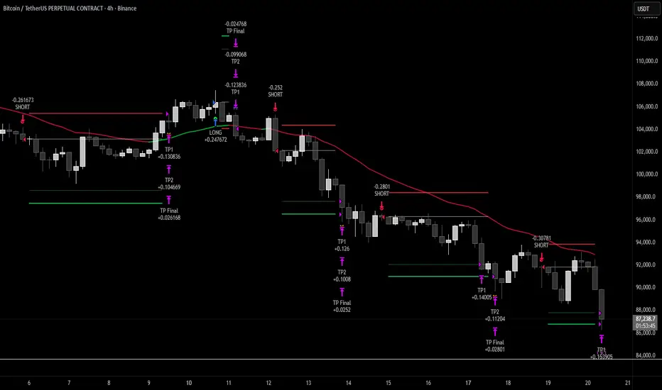
SigmaKernel - AdaptiveSigmaKernel - Adaptive Self-Optimizing Multi-Factor Trading System
SigmaKernel - Adaptive is a self-learning algorithmic trading strategy that combines four distinct analytical dimensions—momentum, market structure, volume flow, and reversal patterns—within a machine-learning-inspired framework that continuously adjusts its own parameters based on realized trading performance. Unlike traditional fixed-parameter strategies that maintain static weightings regardless of market conditions or results, this system implements a feedback loop that tracks which signal types, directional biases, and market conditions produce profitable outcomes, then mathematically adjusts component weightings, minimum score thresholds, position sizing multipliers, and trade spacing requirements to optimize future performance.
The strategy is designed for futures traders operating on prop firm accounts or live capital, incorporating realistic execution mechanics including configurable entry modes (stop breakout orders, limit pullback entries, or market-on-open), commission structures calibrated to retail futures contracts ($0.62 per contract default), one-tick slippage modeling, and professional risk controls including trailing drawdown guards, daily loss limits, and weekly profit targets. The system features universal futures compatibility—it automatically detects and adapts to any futures contract by reading the instrument's tick size and point value directly from the chart, eliminating the need for manual configuration across different markets.
What Makes This Approach Different
Adaptive Weight Optimization System
The core differentiation is the adaptive learning architecture. The strategy maintains four independent scoring components: momentum analysis (using RSI multi-timeframe, MACD histogram, and DMI/ADX), market structure detection (breakout identification via pivot-based support/resistance and moving average positioning), volume flow analysis (Volume Price Trend indicator with standard deviation confirmation), and reversal pattern recognition (oversold/overbought conditions combined with structural levels).
Each component generates a directional score that is multiplied by its current weight. After every closed trade, the system performs a retrospective analysis on the last N trades (configurable Learning Period, default 15 trades) to calculate win rates for each signal type independently. For example, if momentum-driven trades won 65% of the time while reversal trades won only 35%, the adaptive algorithm increases the momentum weight and decreases the reversal weight proportionally. The adjustment formula is:
New_Weight = Current_Weight + (Component_Win_Rate - Average_Win_Rate) × Adaptation_Speed
This creates a self-correcting mechanism where successful signal generators receive more influence in future composite scores, while underperforming components are de-emphasized. The system separately tracks long versus short win rates and applies directional bias corrections—if shorts consistently outperform longs, the strategy applies a 10% reduction to bullish signals to prevent fighting the prevailing market character.
Dynamic Parameter Adjustment
Beyond component weightings, three critical strategy parameters self-adjust based on performance:
Minimum Signal Score: The threshold required to trigger a trade. If overall win rate falls below 45%, the system increments this threshold by 0.10 per adjustment cycle, making the strategy more selective. If win rate exceeds 60%, the threshold decreases to allow more opportunities. This prevents the strategy from overtrading during unfavorable conditions and capitalizes on high-probability environments.
Risk Multiplier: Controls position sizing aggression. When drawdown exceeds 5%, risk per trade reduces by 10% per cycle. When drawdown falls below 2%, risk increases by 5% per cycle. This implements the professional risk management principle of "bet small when losing, bet bigger when winning" algorithmically.
Bars Between Trades: Spacing filter to prevent overtrading. Base value (default 9 bars) multiplies by drawdown factor and losing streak factor. During drawdown or consecutive losses, spacing expands up to 2x to allow market conditions to change before re-entering.
All adaptation operates during live forward-testing or real trading—there is no in-sample optimization applied to historical data. The system learns solely from its own realized trades.
Universal Futures Compatibility
The strategy implements universal futures instrument detection that automatically adapts to any futures contract without requiring manual configuration. Instead of hardcoding specific contract specifications, the system reads three critical values directly from TradingView's symbol information:
Tick Size Detection: Uses `syminfo.mintick` to obtain the minimum price increment for the current instrument. This value varies widely across markets—ES trades in 0.25 ticks, crude oil (CL) in 0.01 ticks, gold (GC) in 0.10 ticks, and treasury futures (ZB) in increments of 1/32nds. The strategy adapts all entry buffer calculations and stop placement logic to the detected tick size.
Point Value Detection: Uses `syminfo.pointvalue` to determine the dollar value per full point of price movement. For ES, one point equals $50; for crude oil, one point equals $1,000; for gold, one point equals $100. This automatic detection ensures accurate P&L calculations and risk-per-contract measurements across all instruments.
Tick Value Calculation: Combines tick size and point value to compute dollar value per tick: Tick_Value = Tick_Size × Point_Value. This derived value drives all position sizing calculations, ensuring the risk management system correctly accounts for each instrument's economic characteristics.
This universal approach means the strategy functions identically on emini indices (ES, MES, NQ, MNQ), micro indices, energy contracts (CL, NG, RB), metals (GC, SI, HG), agricultural futures (ZC, ZS, ZW), treasury futures (ZB, ZN, ZF), currency futures (6E, 6J, 6B), and any other futures contract available on TradingView. No parameter adjustments or instrument-specific branches exist in the code—the adaptation happens automatically through symbol information queries.
Stop-Out Rate Monitoring System
The strategy includes an intelligent stop-out rate tracking system that monitors the percentage of your last 20 trades (or available trades if fewer than 20) that were stopped out. This metric appears in the dashboard's Performance section with color-coded guidance:
Green (<30% stop-out rate): Very few trades are being stopped out. This suggests either your stops are too loose (giving back profits on reversals) or you're in an exceptional trending market. Consider tightening your Stop Loss ATR multiplier to lock in profits more efficiently.
Orange (30-65% stop-out rate): Healthy range. Your stop placement is appropriately sized for current market conditions and the strategy's risk-reward profile. No adjustment needed.
Red (>65% stop-out rate): Too many trades are being stopped out prematurely. Your stops are likely too tight for the current volatility regime. Consider widening your Stop Loss ATR multiplier to give trades more room to develop.
Critical Design Philosophy: Unlike some systems that automatically adjust stops based on performance statistics, this strategy intentionally keeps stop-loss control in the user's hands. Automatic stop adjustment creates dangerous feedback loops—widening stops increases risk per contract, which forces position size reduction, which distorts performance metrics, leading to incorrect adaptations. Instead, the dashboard provides visibility into stop performance, empowering you to make informed manual adjustments when warranted. This preserves the integrity of the adaptive system while giving you the critical data needed for stop optimization.
Execution Kernel Architecture
The entry system offers three distinct execution modes to match trader preference and market character:
StopBreakout Mode: Places buy-stop orders above the prior bar's high (for longs) or sell-stop orders below the prior bar's low (for shorts), plus a 2-tick buffer. This ensures entries only occur when price confirms directional momentum by breaking recent structure. Ideal for trending and momentum-driven markets.
LimitPullback Mode: Places limit orders at a pullback price calculated as: Entry_Price = Close - (ATR × Pullback_Multiplier) for longs, or Close + (ATR × Pullback_Multiplier) for shorts. Default multiplier is 0.5 ATR. This waits for mean-reversion before entering in the signal direction, capturing better prices in volatile or oscillating markets.
MarketNextOpen Mode: Executes at market on the bar immediately following signal generation. This provides fastest execution but sacrifices the filtering effect of requiring price confirmation.
All pending entry orders include a configurable Time-To-Live (TTL, default 6 bars). If an order is not filled within the TTL period, it cancels automatically to prevent stale signals from executing in changed market conditions.
Professional Exit Management
The exit system implements a three-stage progression: initial stop loss, breakeven adjustment, and dynamic trailing stop.
Initial Stop Loss: Calculated as entry price ± (ATR × User_Stop_Multiplier × Volatility_Adjustment). Users have direct control via the Stop Loss ATR multiplier (default 1.25). The system then applies volatility regime adjustments: ×1.2 in high-volatility environments (stops automatically widen), ×0.8 in low volatility (stops tighten), ×1.0 in normal conditions. This ensures stops adapt to market character while maintaining user control over baseline risk tolerance.
Breakeven Trigger: When profit reaches a configurable multiple of initial risk (default 1.0R), the stop loss automatically moves to breakeven (entry price). This locks in zero-loss status once the trade demonstrates favorable movement.
Trailing Stop Activation: When profit reaches the Trail_Trigger_R multiple (default 1.2R), the system cancels the fixed stop and activates a dynamic trailing stop. The trail uses Step and Offset parameters defined in R-multiples. For example, with Trail_Offset_R = 1.0 and Trail_Step_R = 1.5, the stop trails 1.0R behind price and moves in 1.5R increments. This captures extended moves while protecting accumulated profit.
Additional failsafes include maximum time-in-trade (exits after N bars if specified) and end-of-session flatten (automatically closes all positions X minutes before session end to avoid overnight exposure).
Core Calculation Methodology
Signal Component Scoring
Momentum Component:
- Calculates 14-period DMI (Directional Movement Index) with ADX strength filter (trending when ADX > 25)
- Computes three RSI timeframes: fast (7-period), medium (14-period), slow (21-period)
- Analyzes MACD (12/26/9) histogram for directional acceleration
- Bullish momentum: uptrend (DI+ > DI- with ADX > 25) + MACD histogram rising above zero + RSI fast between 50-80 = +1.6 score
- Bearish momentum: downtrend (DI- > DI+ with ADX > 25) + MACD histogram falling below zero + RSI fast between 20-50 = -1.6 score
- Score multiplies by volatility adjustment factor: ×0.8 in high volatility (momentum less reliable), ×1.2 in low volatility (momentum more persistent)
Structure Component:
- Identifies swing highs and lows using 10-bar pivot lookback on both sides
- Maintains most recent swing high as dynamic resistance, most recent swing low as dynamic support
- Detects breakouts: bullish when close crosses above resistance with prior bar below; bearish when close crosses below support with prior bar above
- Breakout score: ±1.0 for confirmed break
- Moving average alignment: +0.5 when price > SMA20 > SMA50 (bullish structure); -0.5 when price < SMA20 < SMA50 (bearish structure)
- Total structure range: -1.5 to +1.5
Volume Component:
- Calculates Volume Price Trend: VPT = Σ [(Close - Close ) / Close × Volume]
- Compares VPT to its 10-period EMA as signal line (similar to MACD logic)
- Computes 20-period volume moving average and standard deviation
- High volume event: current volume > (volume_average + 1× std_dev)
- Bullish volume: VPT > VPT_signal AND high_volume = +1.0
- Bearish volume: VPT < VPT_signal AND high_volume = -1.0
- No score if volume is not elevated (filters out low-conviction moves)
Reversal Component:
- Identifies extreme RSI conditions: RSI slow < 30 (oversold) or > 70 (overbought)
- Requires structural confluence: price at or below support level for bullish reversal; at or above resistance for bearish reversal
- Requires momentum shift: RSI fast must be rising (for bull) or falling (for bear) to confirm reversal in progress
- Bullish reversal: RSI < 30 AND price ≤ support AND RSI rising = +1.0
- Bearish reversal: RSI > 70 AND price ≥ resistance AND RSI falling = -1.0
Composite Score Calculation
Final_Score = (Momentum × Weight_M) + (Structure × Weight_S) + (Volume × Weight_V) + (Reversal × Weight_R)
Initial weights: Momentum = 1.0, Structure = 1.2, Volume = 0.8, Reversal = 0.6
These weights adapt after each trade based on component-specific performance as described above.
The system also applies directional bias adjustment: if recent long trades have significantly lower win rate than shorts, bullish scores multiply by 0.9 to reduce aggressive long entries. Vice versa for underperforming shorts.
Position Sizing Algorithm
The position sizing calculation incorporates multiple confidence factors and automatically scales to any futures contract:
1. Base risk amount = Account_Size × Base_Risk_Percent × Adaptive_Risk_Multiplier
2. Stop distance in price units = ATR × User_Stop_Multiplier × Volatility_Regime_Multiplier × Entry_Buffer
3. Risk per contract = Stop_Distance × Dollar_Per_Point (automatically detected from instrument)
4. Raw position size = Risk_Amount / Risk_Per_Contract
Then applies confidence scaling:
- Signal confidence = min(|Weighted_Score| / Min_Score_Threshold, 2.0) — higher scores receive larger size, capped at 2×
- Direction confidence = Long_Win_Rate (for bulls) or Short_Win_Rate (for bears)
- Type confidence = Win_Rate of dominant signal type (momentum/structure/volume/reversal)
- Total confidence = (Signal_Confidence + Direction_Confidence + Type_Confidence) / 3
Adjusted size = Raw_Size × Total_Confidence × Losing_Streak_Reduction
Losing streak reduction = 0.5 if losing_streak ≥ 5, otherwise 1.0
Universal Maximum Position Calculation: Instead of hardcoded limits per instrument, the system calculates maximum position size as: Max_Contracts = Account_Size / 25000, clamped between 1 and 10 contracts. This means a $50,000 account allows up to 2 contracts, a $100,000 account allows up to 4 contracts, regardless of which futures contract is being traded. This universal approach maintains consistent risk exposure across different instruments while preventing overleveraging.
Final size is rounded to integer and bounded by the calculated maximum.
Session and Risk Management System
Timezone-Aware Session Control
The strategy implements timezone-correct session filtering. Users specify session start hour, end hour, and timezone from 12 supported zones (New York, Chicago, Los Angeles, London, Frankfurt, Moscow, Tokyo, Hong Kong, Shanghai, Singapore, Sydney, UTC). The system converts bar timestamps to the selected timezone before applying session logic.
For split sessions (e.g., Asian session 18:00-02:00), the logic correctly handles time wraparound. Weekend trading can be optionally disabled (default: disabled) to avoid low-liquidity weekend price action.
Multi-Layer Risk Controls
Daily Loss Limit: Strategy ceases all new entries when daily P&L reaches negative threshold (default $2,000). This prevents catastrophic drawdown days. Resets at timezone-corrected day boundary.
Weekly Profit Target: Strategy ceases trading when weekly profit reaches target (default $10,000). This implements the professional principle of "take the win and stop pushing luck." Resets on timezone-corrected Monday.
Maximum Daily Trades: Hard cap on entries per day (default 20) to prevent overtrading during volatile conditions when many signals may generate.
Trailing Drawdown Guard: Optional prop-firm-style trailing stop on account equity. When enabled, if equity drops below (Peak_Equity - Trailing_DD_Amount), all trading halts. This simulates the common prop firm rule where exceeding trailing drawdown results in account termination.
All limits display status in the real-time dashboard, showing "MAX LOSS HIT", "WEEKLY TARGET MET", or "ACTIVE" depending on current state.
How To Use This Strategy
Initial Setup
1. Apply the strategy to your desired futures chart (tested on 5-minute through daily timeframes)
2. The strategy will automatically detect your instrument's specifications—no manual configuration needed for different contracts
3. Configure your account size and risk parameters in the Core Settings section
4. Set your trading session hours and timezone to match your availability
5. Adjust the Stop Loss ATR multiplier based on your risk tolerance (0.8-1.2 for tighter stops, 1.5-2.5 for wider stops)
6. Select your preferred entry execution mode (recommend StopBreakout for beginners)
7. Enable adaptation (recommended) or disable for fixed-parameter operation
8. Review the strategy's Properties in the Strategy Tester settings and verify commission/slippage match your broker's actual costs
The universal futures detection means you can switch between ES, NQ, CL, GC, ZB, or any other futures contract without changing any strategy parameters—the system will automatically adapt its calculations to each instrument's unique specifications.
Dashboard Interpretation
The strategy displays a comprehensive real-time dashboard in the top-right corner showing:
Market State Section:
- Trend: Shows UPTREND/DOWNTREND/CONSOLIDATING/NEUTRAL based on ADX and DMI analysis
- ADX Value: Current trend strength (>25 = strong trend, <20 = consolidating)
- Momentum: BULL/BEAR/NEUTRAL classification with current momentum score
- Volatility: HIGH/LOW/NORMAL regime with ATR percentage of price
Volume Profile Section (Large dashboard only):
- VPT Flow: Directional bias from volume analysis
- Volume Status: HIGH/LOW/NORMAL with relative volume multiplier
Performance Section:
- Daily P&L: Current day's profit/loss with color coding
- Daily Trades: Number of completed trades today
- Weekly P&L: Current week's profit/loss
- Target %: Progress toward weekly profit target
- Stop-Out Rate: Percentage of last 20 trades (or available trades if <20) that were stopped out. Includes all stop types: initial stops, breakeven stops, trailing stops, timeout exits, and EOD flattens. Color coded with actionable guidance:
- Green (<30%): Shows "TIGHTEN" guidance. Very few stop-outs suggests stops may be too loose or exceptional market conditions. Consider reducing Stop Loss ATR multiplier.
- Orange (30-65%): Shows "OK" guidance. Healthy stop-out rate indicating appropriate stop placement for current conditions.
- Red (>65%): Shows "WIDEN" guidance. Too many premature stop-outs. Consider increasing Stop Loss ATR multiplier to give trades more room.
- Status: Overall trading status (ACTIVE/MAX LOSS HIT/WEEKLY TARGET MET/FILTERS ACTIVE)
Adaptive Engine Section:
- Min Score: Current minimum threshold for trade entry (higher = more selective)
- Risk Mult: Current position sizing multiplier (adjusts with performance)
- Bars BTW: Current minimum bars required between trades
- Drawdown: Current drawdown percentage from equity peak
- Weights: M/S/V/R showing current component weightings
Win Rates Section:
- Type: Win rates for Momentum, Structure, Volume, Reversal signal types
- Direction: Win rates for Long vs Short trades
Color coding shows green for >50% win rate, red for <50%
Session Info Section:
- Session Hours: Active trading window with timezone
- Weekend Trading: ENABLED/DISABLED status
- Session Status: ACTIVE/INACTIVE based on current time
Signal Generation and Entry
The strategy generates entries when the weighted composite score exceeds the adaptive minimum threshold (initial value configurable, typically 1.5 to 2.5). Entries display as layered triangle markers on the chart:
- Long Signal: Three green upward triangles below the entry bar
- Short Signal: Three red downward triangles above the entry bar
Triangle tooltip shows the signal score and dominant signal type (MOMENTUM/STRUCTURE/VOLUME/REVERSAL).
Position Management and Stop Optimization
Once entered, the strategy automatically manages the position through its three-stage exit system. Monitor the Stop-Out Rate metric in the dashboard to optimize your stop placement:
If Stop-Out Rate is Green (<30%): You're rarely being stopped out. This could mean:
- Your stops are too loose, allowing trades to give back too much profit on reversals
- You're in an exceptional trending market where tight stops would work better
- Action: Consider reducing your Stop Loss ATR multiplier by 0.1-0.2 to tighten stops and lock in profits more efficiently
If Stop-Out Rate is Orange (30-65%): Optimal range. Your stops are appropriately sized for the strategy's risk-reward profile and current market volatility. No adjustment needed.
If Stop-Out Rate is Red (>65%): You're being stopped out too frequently. This means:
- Your stops are too tight for current market volatility
- Trades need more room to develop before reaching profit targets
- Action: Increase your Stop Loss ATR multiplier by 0.1-0.3 to give trades more breathing room
Remember: The stop-out rate calculation includes all exit types (initial stops, breakeven stops, trailing stops, timeouts, EOD flattens). A trade that reaches breakeven and gets stopped out at entry price counts as a stop-out, even though it didn't lose money. This is intentional—it indicates the stop placement didn't allow the trade to develop into profit.
Optimization Workflow
For traders wanting to customize the strategy for their specific instrument and timeframe:
Week 1-2: Run with defaults, adaptation enabled
Allow the system to execute at least 30-50 trades (the Learning Period plus additional buffer). Monitor which session periods, signal types, and market conditions produce the best results. Observe your stop-out rate—if it's consistently red or green, plan to adjust Stop Loss ATR multiplier after the learning period. Do not adjust parameters yet—let the adaptive system establish baseline performance data.
Week 3-4: Analyze adaptation behavior and optimize stops
Review the dashboard's adaptive weights and win rates. If certain signal types consistently show <40% win rate, consider slightly reducing their base weight. If a particular entry mode produces better fill quality and win rate, switch to that mode. If you notice the minimum score threshold has climbed very high (>3.0), market conditions may not suit the strategy's logic—consider switching instruments or timeframes.
Based on your Stop-Out Rate observations:
- Consistently <30%: Reduce Stop Loss ATR multiplier by 0.2-0.3
- Consistently >65%: Increase Stop Loss ATR multiplier by 0.2-0.4
- Oscillating between zones: Leave stops at default and let volatility regime adjustments handle it
Ongoing: Fine-tune risk and execution
Adjust the following based on your risk tolerance and account type:
- Base Risk Per Trade: 0.5% for conservative, 0.75% for moderate, 1.0% for aggressive
- Stop Loss ATR Multiplier: 0.8-1.2 for tight stops (scalping), 1.5-2.5 for wide stops (swing trading)
- Bars Between Trades: Lower (5-7) for more opportunities, higher (12-20) for more selective
- Entry Mode: Experiment between modes to find best fit for current market character
- Session Hours: Narrow to specific high-performance session windows if certain hours consistently underperform
Never adjust: Do not manually modify the adaptive weights, minimum score, or risk multiplier after the system has begun learning. These parameters are self-optimizing and manual interference defeats the adaptive mechanism.
Parameter Descriptions and Optimization Guidelines
Adaptive Intelligence Group
Enable Self-Optimization (default: true): Master switch for the adaptive learning system. When enabled, component weights, minimum score, risk multiplier, and trade spacing adjust based on realized performance. Disable to run the strategy with fixed parameters (useful for comparing adaptive vs non-adaptive performance).
Learning Period (default: 15 trades): Number of most recent trades to analyze for performance calculations. Shorter values (10-12) adapt more quickly to recent conditions but may overreact to variance. Longer values (20-30) produce more stable adaptations but respond slower to regime changes. For volatile markets, use shorter periods. For stable trends, use longer periods.
Adaptation Speed (default: 0.25): Controls the magnitude of parameter adjustments per learning cycle. Lower values (0.05-0.15) make gradual, conservative changes. Higher values (0.35-0.50) make aggressive adjustments. Faster adaptation helps in rapidly changing markets but increases parameter instability. Start with default and increase only if you observe the system failing to adapt quickly enough to obvious performance patterns.
Performance Memory (default: 100 trades): Maximum number of historical trades stored for analysis. This array size does not affect learning (which uses only Learning Period trades) but provides data for future analytics features including stop-out rate tracking. Higher values consume more memory but provide richer historical dataset. Typical users should not need to modify this.
Core Settings Group
Account Size (default: $50,000): Starting capital for position sizing calculations. This should match your actual account size for accurate risk per trade. The strategy uses this value to calculate dollar risk amounts and determine maximum position size (1 contract per $25,000).
Weekly Profit Target (default: $10,000): When weekly P&L reaches this value, the strategy stops taking new trades for the remainder of the week. This implements a "quit while ahead" rule common in professional trading. Set to a realistic weekly goal—20% of account size per week ($10K on $50K) is very aggressive; 5-10% is more sustainable.
Max Daily Loss (default: $2,000): When daily P&L reaches this negative threshold, strategy stops all new entries for the day. This is your maximum acceptable daily loss. Professional traders typically set this at 2-4% of account size. A $2,000 loss on a $50,000 account = 4%.
Base Risk Per Trade % (default: 0.5%): Initial percentage of account to risk on each trade before adaptive multiplier and confidence scaling. 0.5% is conservative, 0.75% is moderate, 1.0-1.5% is aggressive. Remember that actual risk per trade = Base Risk × Adaptive Risk Multiplier × Confidence Factors, so the realized risk will vary.
Trade Filters Group
Base Minimum Signal Score (default: 1.5): Initial threshold that composite weighted score must exceed to generate a signal. Lower values (1.0-1.5) produce more trades with lower average quality. Higher values (2.0-3.0) produce fewer, higher-quality setups. This value adapts automatically when adaptive mode is enabled, but the base sets the starting point. For trending markets, lower values work well. For choppy markets, use higher values.
Base Bars Between Trades (default: 9): Minimum bars that must elapse after an entry before another signal can trigger. This prevents overtrading and allows previous trades time to develop. Lower values (3-6) suit scalping on lower timeframes. Higher values (15-30) suit swing trading on higher timeframes. This value also adapts based on drawdown and losing streaks.
Max Daily Trades (default: 20): Hard limit on total trades per day regardless of signal quality. This prevents runaway trading during extremely volatile days when many signals may generate. For 5-minute charts, 20 trades/day is reasonable. For 1-hour charts, 5-10 trades/day is more typical.
Session Group
Session Start Hour (default: 5): Hour (0-23 format) when trading is allowed to begin, in the timezone specified. For US futures trading in Chicago time, session typically starts at 5:00 or 6:00 PM (17:00 or 18:00) Sunday evening.
Session End Hour (default: 17): Hour when trading stops and no new entries are allowed. For US equity index futures, regular session ends at 4:00 PM (16:00) Central Time.
Allow Weekend Trading (default: false): Whether strategy can trade on Saturday/Sunday. Most futures have low volume on weekends; keeping this disabled is recommended unless you specifically trade Sunday evening open.
Session Timezone (default: America/Chicago): Timezone for session hour interpretation. Select your local timezone or the timezone of your instrument's primary exchange. This ensures session logic aligns with your intended trading hours.
Prop Guards Group
Trailing Drawdown Guard (default: false): Enables prop-firm-style trailing maximum drawdown. When enabled, if equity drops below (Peak Equity - Trailing DD Amount), all trading halts for the remainder of the backtest/live session. This simulates rules used by funded trader programs where exceeding trailing drawdown terminates the account.
Trailing DD Amount (default: $2,500): Dollar amount of drawdown allowed from equity peak. If your equity reaches $55,000, the trailing stop sets at $52,500. If equity then drops to $52,499, the guard triggers and trading ceases.
Execution Kernel Group
Entry Mode (default: StopBreakout):
- StopBreakout: Places stop orders above/below signal bar requiring price confirmation
- LimitPullback: Places limit orders at pullback prices seeking better fills
- MarketNextOpen: Executes immediately at market on next bar
Limit Offset (default: 0.5x ATR): For LimitPullback mode, how far below/above current price to place the limit order. Smaller values (0.3-0.5) seek minor pullbacks. Larger values (0.8-1.2) wait for deeper retracements but may miss trades.
Entry TTL (default: 6 bars, 0=off): Bars an entry order remains pending before cancelling. Shorter values (3-4) keep signals fresh. Longer values (8-12) allow more time for fills but risk executing stale signals. Set to 0 to disable TTL (orders remain active indefinitely until filled or opposite signal).
Exits Group
Stop Loss (default: 1.25x ATR): Base stop distance as a multiple of the 14-period ATR. This is your primary risk control parameter and directly impacts your stop-out rate. Lower values (0.8-1.0) create tighter stops that reduce risk per trade but may get stopped out prematurely in volatile conditions—expect stop-out rates above 65% (red zone). Higher values (1.5-2.5) give trades more room to breathe but increase risk per contract—expect stop-out rates below 30% (green zone). The system applies additional volatility regime adjustments on top of this base: ×1.2 in high volatility environments (stops widen automatically), ×0.8 in low volatility (stops tighten), ×1.0 in normal conditions. For scalping on lower timeframes, use 0.8-1.2. For swing trading on higher timeframes, use 1.5-2.5. Monitor the Stop-Out Rate metric in the dashboard and adjust this parameter to keep it in the healthy 30-65% orange zone.
Move to Breakeven at (default: 1.0R): When profit reaches this multiple of initial risk, stop moves to breakeven. 1.0R means after price moves in your favor by the distance you risked, you're protected at entry price. Lower values (0.5-0.8R) lock in breakeven faster. Higher values (1.5-2.0R) allow more room before protection.
Start Trailing at (default: 1.2R): When profit reaches this multiple, the fixed stop transitions to a dynamic trailing stop. This should be greater than the BE trigger. Values typically range 1.0-2.0R depending on how much profit you want secured before trailing activates.
Trail Offset (default: 1.0R): How far behind price the trailing stop follows. Tighter offsets (0.5-0.8R) protect profit more aggressively but may exit prematurely. Wider offsets (1.5-2.5R) allow more room for profit to run but risk giving back more on reversals.
Trail Step (default: 1.5R): How far price must move in profitable direction before the stop advances. Smaller steps (0.5-1.0R) move the stop more frequently, tightening protection continuously. Larger steps (2.0-3.0R) move the stop less often, giving trades more breathing room.
Max Bars In Trade (default: 0=off): Maximum bars allowed in a position before forced exit. This prevents trades from "going stale" during periods of no meaningful price action. For 5-minute charts, 50-100 bars (4-8 hours) is reasonable. For daily charts, 5-10 bars (1-2 weeks) is typical. Set to 0 to disable.
Flatten near Session End (default: true): Whether to automatically close all positions as session end approaches. Recommended to avoid carrying positions into off-hours with low liquidity.
Minutes before end (default: 5): How many minutes before session end to flatten. 5-15 minutes provides buffer for order execution before the session boundary.
Visual Effects Configuration Group
Dashboard Size (default: Normal): Controls information density in the dashboard. Small shows only critical metrics (excludes stop-out rate). Normal shows comprehensive data including stop-out rate. Large shows all available metrics including weights, session info, and volume analysis. Larger sizes consume more screen space but provide complete visibility.
Show Quantum Field (default: true): Displays animated grid pattern on the chart indicating market state. Disable if you prefer cleaner charts or experience performance issues on lower-end hardware.
Show Wick Pressure Lines (default: true): Draws dynamic lines from bars with extreme wicks, indicating potential support/resistance or liquidity absorption zones. Disable for simpler visualization.
Show Morphism Energy Beams (default: true): Displays directional beams showing momentum energy flow. Beams intensify during strong trends. Disable if you find this visually distracting.
Show Order Flow Clouds (default: true): Draws translucent boxes representing volume flow bullish/bearish bias. Disable for cleaner price action visibility.
Show Fractal Grid (default: true): Displays multi-timeframe support/resistance levels based on fractal price structure at 10/20/30/40/50 bar periods. Disable if you only want to see primary pivot levels.
Glow Intensity (default: 4): Controls the brightness and thickness of visual effects. Lower values (1-2) for subtle visualization. Higher values (7-10) for maximum visibility but potentially cluttered charts.
Color Theme (default: Cyber): Visual color scheme. Cyber uses cyan/magenta futuristic colors. Quantum uses aqua/purple. Matrix uses green/red terminal style. Aurora uses pastel pink/purple gradient. Choose based on personal preference and monitor calibration.
Show Watermark (default: true): Displays animated watermark at bottom of chart with creator credit and current P&L. Disable if you want completely clean charts or need screen space.
Performance Characteristics and Best Use Cases
Optimal Conditions
This strategy performs best in markets exhibiting:
Trending phases with periodic pullbacks: The combination of momentum and structure components excels when price establishes directional bias but provides retracement opportunities for entries. Markets with 60-70% trending bars and 30-40% consolidation produce the highest win rates.
Medium to high volatility: The ATR-based stop sizing and dynamic risk adjustment require sufficient price movement to generate meaningful profit relative to risk. Instruments with 2-4% daily ATR relative to price work well. Extremely low volatility (<1% daily ATR) generates too many scratch trades.
Clear volume patterns: The VPT volume component adds significant edge when volume expansions align with directional moves. Instruments and timeframes where volume data reflects actual transaction flow (versus tick volume proxies) perform better.
Regular session structure: Futures markets with defined opening and closing hours, consistent liquidity throughout the session, and clear overnight/day session separation allow the session controls and time-based failsafes to function optimally.
Sufficient liquidity for stop execution: The stop breakout entry mode requires that stop orders can fill without significant slippage. Highly liquid contracts work better than illiquid instruments where stop orders may face adverse fills.
Suboptimal Conditions
The strategy may struggle with:
Extreme chop with no directional persistence: When ADX remains below 15 for extended periods and price oscillates rapidly without establishing trends, the momentum component generates conflicting signals. Win rate typically drops below 40% in these conditions, triggering the adaptive system to increase minimum score thresholds until conditions improve. Stop-out rates may also spike into the red zone.
Gap-heavy instruments: Markets with frequent overnight gaps disrupt the continuous price assumptions underlying ATR stops and EMA-based structure analysis. Gaps can also cause stop orders to fill at prices far from intended levels, distorting stop-out rate metrics.
Very low timeframes with excessive noise: On 1-minute or tick charts, the signal components react to micro-structure noise rather than meaningful price swings. The strategy works best on 5-minute through daily timeframes where price movements reflect actual order flow shifts.
Extended low-volatility compression: During historically low volatility periods, profit targets become difficult to reach before mean-reversion occurs. The trail offset, even when set to minimum, may be too wide for the compressed price environment. Stop-out rates may drop to green zone indicating stops should be tightened.
Parabolic moves or climactic exhaustion: Vertical price advances or selloffs where price moves multiple ATRs in single bars can trigger momentum signals at exhaustion points. The structure and reversal components attempt to filter these, but extreme moves may override normal logic.
The adaptive learning system naturally reduces signal frequency and position sizing during unfavorable conditions. If you observe multiple consecutive days with zero trades and "FILTERS ACTIVE" status, this indicates the strategy has self-adjusted to avoid poor conditions rather than forcing trades.
Instrument Recommendations
Emini Index Futures (ES, MES, NQ, MNQ, YM, RTY): Excellent fit. High liquidity, clear volatility patterns, strong volume signals, defined session structure. These instruments have been extensively tested and the universal detection handles all contract specifications automatically.
Micro Index Futures (MES, MNQ, M2K, MYM): Excellent fit for smaller accounts. Same market characteristics as the standard eminis but with reduced contract sizes allowing proper risk management on accounts below $50,000.
Energy Futures (CL, NG, RB, HO): Good to mixed fit. Crude oil (CL) works well due to strong trends and reasonable volatility. Natural gas (NG) can be extremely volatile—consider reducing Base Risk to 0.3-0.4% and increasing Stop Loss ATR multiplier to 1.8-2.2 for NG. The strategy automatically detects the $10/tick value for CL and adjusts position sizing accordingly.
Metal Futures (GC, SI, HG, PL): Good fit. Gold (GC) and silver (SI) exhibit clear trending behavior and work well with the momentum/structure components. The strategy automatically handles the different point values ($100/point for gold, $5,000/point for silver).
Agricultural Futures (ZC, ZS, ZW, ZL): Good fit. Grain futures often trend strongly during seasonal periods. The strategy handles the unique tick sizes (1/4 cent increments) and point values ($50/point for corn/wheat, $60/point for soybeans) automatically.
Treasury Futures (ZB, ZN, ZF, ZT): Good fit for trending rates environments. The strategy automatically handles the fractional tick sizing (32nds for ZB/ZN, halves of 32nds for ZF/ZT) through the universal detection system.
Currency Futures (6E, 6J, 6B, 6A, 6C): Good fit. Major currency pairs exhibit smooth trending behavior. The strategy automatically detects point values which vary significantly ($12.50/tick for 6E, $12.50/tick for 6J, $6.25/tick for 6B).
Cryptocurrency Futures (BTC, ETH, MBT, MET): Mixed fit. These markets have extreme volatility requiring parameter adjustment. Increase Base Risk to 0.8-1.2% and Stop Loss ATR multiplier to 2.0-3.0 to account for wider stop distances. Enable 24-hour trading and weekend trading as these markets have no traditional sessions.
The universal futures compatibility means you can apply this strategy to any of these markets without code modification—simply open the chart of your desired contract and the strategy will automatically configure itself to that instrument's specifications.
Important Disclaimers and Realistic Expectations
This is a sophisticated trading strategy that combines multiple analytical methods within an adaptive framework designed for active traders who will monitor performance and market conditions. It is not a "set and forget" fully automated system, nor should it be treated as a guaranteed profit generator.
Backtesting Realism and Limitations
The strategy includes realistic trading costs and execution assumptions:
- Commission: $0.62 per contract per side (accurate for many retail futures brokers)
- Slippage: 1 tick per entry and exit (conservative estimate for liquid futures)
- Position sizing: Realistic risk percentages and maximum contract limits based on account size
- No repainting: All calculations use confirmed bar data only—signals do not change retroactively
However, backtesting cannot fully capture live trading reality:
- Order fill delays: In live trading, stop and limit orders may not fill instantly at the exact tick shown in backtest
- Volatile periods: During high volatility or low liquidity (news events, rollover days, pre-holidays), slippage may exceed the 1-tick assumption significantly
- Gap risk: The backtest assumes stops fill at stop price, but gaps can cause fills far beyond intended exit levels
- Psychological factors: Seeing actual capital at risk creates emotional pressures not present in backtesting, potentially leading to premature manual intervention
The strategy's backtest results should be viewed as best-case scenarios. Real trading will typically produce 10-30% lower returns than backtest due to the above factors.
Risk Warnings
All trading involves substantial risk of loss. The adaptive learning system can improve parameter selection over time, but it cannot predict future price movements or guarantee profitable performance. Past wins do not ensure future wins.
Losing streaks are inevitable. Even with a 60% win rate, you will encounter sequences of 5, 6, or more consecutive losses due to normal probability distributions. The strategy includes losing streak detection and automatic risk reduction, but you must have sufficient capital to survive these drawdowns.
Market regime changes can invalidate learned patterns. If the strategy learns from 50 trades during a trending regime, then the market shifts to a ranging regime, the adapted parameters may initially be misaligned with the new environment. The system will re-adapt, but this transition period may produce suboptimal results.
Prop firm traders: understand your specific rules. Every prop firm has different rules regarding maximum drawdown, daily loss limits, consistency requirements, and prohibited trading behaviors. While this strategy includes common prop guardrails, you must verify it complies with your specific firm's rules and adjust parameters accordingly.
Never risk capital you cannot afford to lose. This strategy can produce substantial drawdowns, especially during learning periods or market regime shifts. Only trade with speculative capital that, if lost, would not impact your financial stability.
Recommended Usage
Paper trade first: Run the strategy on a simulated account for at least 50 trades or 1 month before committing real capital. Observe how the adaptive system behaves, identify any patterns in losing trades, monitor your stop-out rate trends, and verify your understanding of the entry/exit mechanics.
Start with minimum position sizing: When transitioning to live trading, reduce the Base Risk parameter to 0.3-0.4% initially (vs 0.5-1.0% in testing) to reduce early impact while the system learns your live broker's execution characteristics.
Monitor daily, but do not micromanage: Check the dashboard daily to ensure the strategy is operating normally and risk controls have not triggered unexpectedly. Pay special attention to the Stop-Out Rate metric—if it remains in the red or green zones for multiple days, adjust your Stop Loss ATR multiplier accordingly. However, resist the urge to manually adjust adaptive weights or disable trades based on short-term performance. Allow the adaptive system at least 30 trades to establish patterns before making manual changes.
Combine with other analysis: While this strategy can operate standalone, professional traders typically use systematic strategies as one component of a broader approach. Consider using the strategy for trade execution while applying your own higher-timeframe analysis or fundamental view for trade filtering or sizing adjustments.
Keep a trading journal: Document each week's results, note market conditions (trending vs ranging, high vs low volatility), record stop-out rates and any Stop Loss ATR adjustments you made, and document any manual interventions. Over time, this journal will help you identify conditions where the strategy excels versus struggles, allowing you to selectively enable or disable trading during certain environments.
Technical Implementation Notes
All calculations execute on closed bars only (`calc_on_every_tick=false`) ensuring that signals and values do not repaint. Once a bar closes and a signal generates, that signal is permanent in the history.
The strategy uses fixed-quantity position sizing (`default_qty_type=strategy.fixed, default_qty_value=1`) with the actual contract quantity determined by the position sizing function and passed to the entry commands. This approach provides maximum control over risk allocation.
Order management uses Pine Script's native `strategy.entry()` and `strategy.exit()` functions with appropriate parameters for stops, limits, and trailing stops. All orders include explicit from_entry references to ensure they apply to the correct position.
The adaptive learning arrays (trade_returns, trade_directions, trade_types, trade_hours, trade_was_stopped) are maintained as circular buffers capped at PERFORMANCE_MEMORY size (default 100 trades). When a new trade closes, its data is added to the beginning of the array using `array.unshift()`, and the oldest trade is removed using `array.pop()` if capacity is exceeded. The stop-out tracking system analyzes the trade_was_stopped array to calculate the rolling percentage displayed in the dashboard.
Dashboard rendering occurs only on the confirmed bar (`barstate.isconfirmed`) to minimize computational overhead. The table is pre-created with sufficient rows for the selected dashboard size and cells are populated with current values each update.
Visual effects (fractal grid, wick pressure, morphism beams, order flow clouds, quantum field) recalculate on each bar for real-time chart updates. These are computationally intensive—if you experience chart lag, disable these visual components. The core strategy logic continues to function identically regardless of visual settings.
Timezone conversions use Pine Script's built-in timezone parameter on the `hour()`, `minute()`, and `dayofweek()` functions. This ensures session logic and daily/weekly resets occur at correct boundaries regardless of the chart's default timezone or the server's timezone.
The universal futures detection queries `syminfo.mintick` and `syminfo.pointvalue` on each strategy initialization to obtain the current instrument's specifications. These values remain constant throughout the strategy's execution on a given chart but automatically update when the strategy is applied to a different instrument.
The strategy has been tested on TradingView across timeframes from 5-minute through daily and across multiple futures instrument types including equity indices, energy, metals, agriculture, treasuries, and currencies. It functions identically on all instruments due to the percentage-based risk model and ATR-relative calculations which adapt automatically to price scale and volatility, combined with the universal futures detection system that handles contract-specific specifications.

AM Range Sniper [jmaxxx]AM Range Sniper
Overview
AM Range Sniper is a sophisticated morning session trading strategy designed for Micro E-mini Nasdaq-100 Index Futures (MNQ). This strategy capitalizes on the critical 8:30-9:30 AM EST range formation period, implementing precise entry and exit mechanics with advanced risk management.
Key Features
🕐 Time-Based Range Analysis
Range Definition: Automatically identifies and tracks the 8:30-9:30 AM EST range
Trading Window: Active trading from 9:30 AM to 11:00 AM EST (extended for second chance trades)
Session Management: Daily reset ensures clean state for each trading session
🎯 Multiple Entry Patterns
Breakthrough/Retest: Captures price breakthroughs above range with retest opportunities
Long/Short Opportunities: Comprehensive coverage of both directional moves
Breakdown: Identifies bearish breakdowns below range support
Break Up: Detects bullish breakups above range resistance
Range Sweeps: Monitors for range high/low sweeps with reversal entries
⚡ Advanced Risk Management
Configurable Stop Losses: Tick-based stop losses for each trade type
Take Profit Targets: Automatic target calculations based on range size
Hard Close Protection: Automatic position closure at 4 PM EST
Second Chance Feature: Optional second trade opportunity if first trade loses
🔧 Professional Features
Visual Stop Loss Lines: Real-time stop loss visualization on chart
Debug Information Panel: Comprehensive status monitoring
Alert Integration: Customizable alert messages for entries/exits
Flexible Time Settings: Adjustable for different timezones
Strategy Logic
Range Formation (8:30-9:30 AM)
The strategy monitors the first hour of trading to establish the day's range. This range serves as the foundation for all subsequent trading decisions.
Entry Conditions
Breakthrough: Price breaks above range high with retest rejection
Breakdown: Price breaks below range low with confirmed bearish momentum
Break Up: Price breaks above range high with strong bullish confirmation
Sweep Entries: Range high/low sweeps followed by reversal signals
Risk Management
Stop Loss: Configurable tick-based stops for each trade type
Take Profit: 1.5x range size targets for breakdown/breakup trades
Position Sizing: Percentage-based position sizing
Session Limits: Maximum 2 trades per session (with second chance feature)
Settings & Customization
Core Parameters
Enable/disable individual entry patterns
Configurable stop loss levels (1-500 ticks)
Second chance feature toggle
Previous day level integration
Visual Customization
Customizable stop loss colors and widths
Debug panel visibility
Range line styling
Alert Configuration
Custom entry/exit alert messages
***** Automate With *****
APEX
NinjaTrader
Crosstrade.io ( promo code JMAXXX )
Performance & Reliability
Precision Focused: Waits for high-probability setups
Risk-Aware: Comprehensive stop loss and position management
Session-Based: Clean daily resets prevent carryover issues
Professional Grade: Designed for serious traders
Ideal For
Day Traders: Morning session specialists
Futures Traders: MNQ and similar instruments
Range Traders: Traders who capitalize on range breakouts
Risk-Conscious Traders: Those who prioritize risk management
Disclaimer
This strategy is for educational and informational purposes. Past performance does not guarantee future results. Always test thoroughly on historical data and paper trading before live implementation. Risk management is crucial - never risk more than you can afford to lose.
Created by jmaxxx - Professional trading strategy developer
For questions, feedback, or customization requests, please leave a comment below.
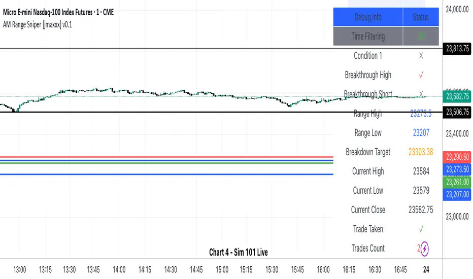
Machine Learning: SuperTrend Strategy TP/SL [YinYangAlgorithms]The SuperTrend is a very useful Indicator to display when trends have shifted based on the Average True Range (ATR). Its underlying ideology is to calculate the ATR using a fixed length and then multiply it by a factor to calculate the SuperTrend +/-. When the close crosses the SuperTrend it changes direction.
This Strategy features the Traditional SuperTrend Calculations with Machine Learning (ML) and Take Profit / Stop Loss applied to it. Using ML on the SuperTrend allows for the ability to sort data from previous SuperTrend calculations. We can filter the data so only previous SuperTrends that follow the same direction and are within the distance bounds of our k-Nearest Neighbour (KNN) will be added and then averaged. This average can either be achieved using a Mean or with an Exponential calculation which puts added weight on the initial source. Take Profits and Stop Losses are then added to the ML SuperTrend so it may capitalize on Momentum changes meanwhile remaining in the Trend during consolidation.
By applying Machine Learning logic and adding a Take Profit and Stop Loss to the Traditional SuperTrend, we may enhance its underlying calculations with potential to withhold the trend better. The main purpose of this Strategy is to minimize losses and false trend changes while maximizing gains. This may be achieved by quick reversals of trends where strategic small losses are taken before a large trend occurs with hopes of potentially occurring large gain. Due to this logic, the Win/Loss ratio of this Strategy may be quite poor as it may take many small marginal losses where there is consolidation. However, it may also take large gains and capitalize on strong momentum movements.
Tutorial:
In this example above, we can get an idea of what the default settings may achieve when there is momentum. It focuses on attempting to hit the Trailing Take Profit which moves in accord with the SuperTrend just with a multiplier added. When momentum occurs it helps push the SuperTrend within it, which on its own may act as a smaller Trailing Take Profit of its own accord.
We’ve highlighted some key points from the last example to better emphasize how it works. As you can see, the White Circle is where profit was taken from the ML SuperTrend simply from it attempting to switch to a Bullish (Buy) Trend. However, that was rejected almost immediately and we went back to our Bearish (Sell) Trend that ended up resulting in our Take Profit being hit (Yellow Circle). This Strategy aims to not only capitalize on the small profits from SuperTrend to SuperTrend but to also capitalize when the Momentum is so strong that the price moves X% away from the SuperTrend and is able to hit the Take Profit location. This Take Profit addition to this Strategy is crucial as momentum may change state shortly after such drastic price movements; and if we were to simply wait for it to come back to the SuperTrend, we may lose out on lots of potential profit.
If you refer to the Yellow Circle in this example, you’ll notice what was talked about in the Summary/Overview above. During periods of consolidation when there is little momentum and price movement and we don’t have any Stop Loss activated, you may see ‘Signal Flashing’. Signal Flashing is when there are Buy and Sell signals that keep switching back and forth. During this time you may be taking small losses. This is a normal part of this Strategy. When a signal has finally been confirmed by Momentum, is when this Strategy shines and may produce the profit you desire.
You may be wondering, what causes these jagged like patterns in the SuperTrend? It's due to the ML logic, and it may be a little confusing, but essentially what is happening is the Fast Moving SuperTrend and the Slow Moving SuperTrend are creating KNN Min and Max distances that are extreme due to (usually) parabolic movement. This causes fewer values to be added to and averaged within the ML and causes less smooth and more exponential drastic movements. This is completely normal, and one of the perks of using k-Nearest Neighbor for ML calculations. If you don’t know, the Min and Max Distance allowed is derived from the most recent(0 index of data array) to KNN Length. So only SuperTrend values that exhibit distances within these Min/Max will be allowed into the average.
Since the KNN ML logic can cause these exponential movements in the SuperTrend, they likewise affect its Take Profit. The Take Profit may benefit from this movement like displayed in the example above which helped it claim profit before then exhibiting upwards movement.
By default our Stop Loss Multiplier is kept quite low at 0.0000025. Keeping it low may help to reduce some Signal Flashing while not taking extra losses more so than not using it at all. However, if we increase it even more to say 0.005 like is shown in the example above. It can really help the trend keep momentum. Please note, although previous results don’t imply future results, at 0.0000025 Stop Loss we are currently exhibiting 69.27% profit while at 0.005 Stop Loss we are exhibiting 33.54% profit. This just goes to show that although there may be less Signal Flashing, it may not result in more profit.
We will conclude our Tutorial here. Hopefully this has given you some insight as to how Machine Learning, combined with Trailing Take Profit and Stop Loss may have positive effects on the SuperTrend when turned into a Strategy.
Settings:
SuperTrend:
ATR Length: ATR Length used to create the Original Supertrend.
Factor: Multiplier used to create the Original Supertrend.
Stop Loss Multiplier: 0 = Don't use Stop Loss. Stop loss can be useful for helping to prevent false signals but also may result in more loss when hit and less profit when switching trends.
Take Profit Multiplier: Take Profits can be useful within the Supertrend Strategy to stop the price reverting all the way to the Stop Loss once it's been profitable.
Machine Learning:
Only Factor Same Trend Direction: Very useful for ensuring that data used in KNN is not manipulated by different SuperTrend Directional data. Please note, it doesn't affect KNN Exponential.
Rationalized Source Type: Should we Rationalize only a specific source, All or None?
Machine Learning Type: Are we using a Simple ML Average, KNN Mean Average, KNN Exponential Average or None?
Machine Learning Smoothing Type: How should we smooth our Fast and Slow ML Datas to be used in our KNN Distance calculation? SMA, EMA or VWMA?
KNN Distance Type: We need to check if distance is within the KNN Min/Max distance, which distance checks are we using.
Machine Learning Length: How far back is our Machine Learning going to keep data for.
k-Nearest Neighbour (KNN) Length: How many k-Nearest Neighbours will we account for?
Fast ML Data Length: What is our Fast ML Length?? This is used with our Slow Length to create our KNN Distance.
Slow ML Data Length: What is our Slow ML Length?? This is used with our Fast Length to create our KNN Distance.
If you have any questions, comments, ideas or concerns please don't hesitate to contact us.
HAPPY TRADING!
[blackcat] L1 MartinGale Scalping Strategy**MartinGale Strategy** is a popular money management strategy used in trading. It is commonly applied in situations where the trader aims to recover from a losing streak by increasing the position size after each loss.
In the MartinGale Strategy, after a losing trade, the trader doubles the position size for the next trade. This is done in the hopes that a winning trade will eventually occur, which will not only recover the previous losses but also generate a profit.
The idea behind the MartinGale Strategy is to take advantage of the law of averages. By increasing the position size after each loss, the strategy assumes that eventually, a winning trade will occur, which will not only cover the previous losses but also generate a profit. This can be especially appealing for traders looking for a quick recovery from a losing streak.
However, it is important to note that the MartinGale Strategy carries significant risks. If a trader experiences a prolonged losing streak or lacks sufficient capital, the strategy can lead to substantial losses. The strategy's reliance on the assumption of a winning trade can be dangerous, as there is no guarantee that a winning trade will occur within a certain timeframe.
Traders considering implementing the MartinGale Strategy should carefully assess their risk tolerance and thoroughly understand the potential drawbacks. It is crucial to have a solid risk management plan in place to mitigate potential losses. Additionally, traders should be aware that the strategy may not be suitable for all market conditions and may require adjustments based on market volatility.
In summary, the MartinGale Strategy is a money management strategy that involves increasing the position size after each loss in an attempt to recover from a losing streak. While it can offer the potential for quick recovery, it also comes with significant risks that traders should carefully consider before implementing it in their trading approach.
The MartinGale Scalping Strategy is a trading strategy designed to generate profits through frequent trades. It utilizes a combination of moving average crossovers and crossunders to generate entry and exit signals. The strategy is implemented in TradingView's Pine Script language.
The strategy begins by defining input variables such as take profit and stop loss levels, as well as the trading mode (long, short, or bidirectional). It then sets a rule to allow only long entries if the trading mode is set to "Long".
The strategy logic is defined using SMA (Simple Moving Average) crossover and crossunder signals. It calculates a short-term SMA (SMA3) and a longer-term SMA (SMA8), and plots them on the chart. The crossoverSignal and crossunderSignal variables are used to track the occurrence of the crossover and crossunder events, while the crossoverState and crossunderState variables determine the state of the crossover and crossunder conditions.
The strategy execution is based on the current position size. If the position size is zero (no open positions), the strategy checks for crossover and crossunder events. If a crossover event occurs and the trading mode allows long entries, a long position is entered. The entry price, stop price, take profit price, and stop loss price are calculated based on the current close price and the SMA8 value. Similarly, if a crossunder event occurs and the trading mode allows short entries, a short position is entered with the corresponding price calculations.
If there is an existing long position and the current close price reaches either the take profit price or the stop loss price, and a crossunder event occurs, the long position is closed. The entry price, stop price, take profit price, and stop loss price are reset to zero.
Likewise, if there is an existing short position and the current close price reaches either the take profit price or the stop loss price, and a crossover event occurs, the short position is closed and the price variables are reset.
The strategy also plots entry and exit points on the chart using plotshape function. It displays a triangle pointing up for a buy entry, a triangle pointing down for a buy exit, a triangle pointing down for a sell entry, and a triangle pointing up for a sell exit.
Overall, the MartinGale Scalping Strategy aims to capture small profits by taking advantage of short-term moving average crossovers and crossunders. It incorporates risk management through take profit and stop loss levels, and allows for different trading modes to accommodate different market conditions.

GKD-BT Baseline Backtest [Loxx]The Giga Kaleidoscope GKD-BT Baseline Backtest is a backtesting module included in Loxx's "Giga Kaleidoscope Modularized Trading System."
█ GKD-BT Baseline Backtest
The GKD-BT Baseline Backtest allows traders to backtest the Regular and Stepped baselines used in the GKD trading system. This module includes 65+ moving averages and 15+ types of volatility to choose from.
Additionally, this backtest module provides the option to test the GKD-B indicator with 1 to 3 take profits and 1 stop loss. The Trading backtest allows for the use of 1 to 3 take profits, while the Full backtest is limited to 1 take profit. The Trading backtest also offers the capability to apply a trailing take profit.
In terms of the percentage of trade removed at each take profit, this backtest module has the following hardcoded values:
Take profit 1: 50% of the trade is removed
Take profit 2: 25% of the trade is removed
Take profit 3: 25% of the trade is removed
Stop loss: 100% of the trade is removed
After each take profit is achieved, the stop loss level is adjusted. When take profit 1 is reached, the stop loss is moved to the entry point. Similarly, when take profit 2 is reached, the stop loss is shifted to take profit 1. The trailing take profit feature comes into play after take profit 2 or take profit 3, depending on the number of take profits selected in the settings. The trailing take profit is always activated on the final take profit when 2 or more take profits are chosen.
The backtest also offers the capability to restrict by a specific date range, allowing for simulated forward testing based on past data. Additionally, users have the option to display or hide a trading panel that provides relevant information about the backtest, statistics, and the current trade. It is also possible to activate alerts and toggle sections of the trading panel on or off. On the chart, historical take profit and stop loss levels are represented by horizontal lines overlaid for reference.
This backtest also includes an optional GKD-E Exit indicator that can be used to test early exits.
The GKD system utilizes volatility-based take profits and stop losses. Each take profit and stop loss is calculated as a multiple of volatility. You can change the values of the multipliers in the settings as well.
To utilize this strategy, follow these steps:
1. (Required) Import the value "Input into NEW GKD-BT Backtest" from the GKD-B Baseline indicator into the GKD-BT Baseline Backtest field "Import GKD-B Baseline"
2. (Optional) Import the value "Input into NEW GKD-BT Backtest" from the GKD-E Exit indicator into the GKD-BT Baseline Backtest field "Import GKD-E Exit". You can toggle the Exit on or off using the "Activate GKD-E Exit" option.
Baselines that are compatible with this backtest module:
GKD-B Baseline
GKD-B Stepped Baseline
Volatility Types Included
17 types of volatility are included in this indicator
Close-to-Close
Parkinson
Garman-Klass
Rogers-Satchell
Yang-Zhang
Garman-Klass-Yang-Zhang
Exponential Weighted Moving Average
Standard Deviation of Log Returns
Pseudo GARCH(2,2)
Average True Range
True Range Double
Standard Deviation
Adaptive Deviation
Median Absolute Deviation
Efficiency-Ratio Adaptive ATR
Mean Absolute Deviation
Static Percent
█ Giga Kaleidoscope Modularized Trading System
Core components of an NNFX algorithmic trading strategy
The NNFX algorithm is built on the principles of trend, momentum, and volatility. There are six core components in the NNFX trading algorithm:
1. Volatility - price volatility; e.g., Average True Range, True Range Double, Close-to-Close, etc.
2. Baseline - a moving average to identify price trend
3. Confirmation 1 - a technical indicator used to identify trends
4. Confirmation 2 - a technical indicator used to identify trends
5. Continuation - a technical indicator used to identify trends
6. Volatility/Volume - a technical indicator used to identify volatility/volume breakouts/breakdown
7. Exit - a technical indicator used to determine when a trend is exhausted
8. Metamorphosis - a technical indicator that produces a compound signal from the combination of other GKD indicators*
*(not part of the NNFX algorithm)
What is Volatility in the NNFX trading system?
In the NNFX (No Nonsense Forex) trading system, ATR (Average True Range) is typically used to measure the volatility of an asset. It is used as a part of the system to help determine the appropriate stop loss and take profit levels for a trade. ATR is calculated by taking the average of the true range values over a specified period.
True range is calculated as the maximum of the following values:
-Current high minus the current low
-Absolute value of the current high minus the previous close
-Absolute value of the current low minus the previous close
ATR is a dynamic indicator that changes with changes in volatility. As volatility increases, the value of ATR increases, and as volatility decreases, the value of ATR decreases. By using ATR in NNFX system, traders can adjust their stop loss and take profit levels according to the volatility of the asset being traded. This helps to ensure that the trade is given enough room to move, while also minimizing potential losses.
Other types of volatility include True Range Double (TRD), Close-to-Close, and Garman-Klass
What is a Baseline indicator?
The baseline is essentially a moving average, and is used to determine the overall direction of the market.
The baseline in the NNFX system is used to filter out trades that are not in line with the long-term trend of the market. The baseline is plotted on the chart along with other indicators, such as the Moving Average (MA), the Relative Strength Index (RSI), and the Average True Range (ATR).
Trades are only taken when the price is in the same direction as the baseline. For example, if the baseline is sloping upwards, only long trades are taken, and if the baseline is sloping downwards, only short trades are taken. This approach helps to ensure that trades are in line with the overall trend of the market, and reduces the risk of entering trades that are likely to fail.
By using a baseline in the NNFX system, traders can have a clear reference point for determining the overall trend of the market, and can make more informed trading decisions. The baseline helps to filter out noise and false signals, and ensures that trades are taken in the direction of the long-term trend.
What is a Confirmation indicator?
Confirmation indicators are technical indicators that are used to confirm the signals generated by primary indicators. Primary indicators are the core indicators used in the NNFX system, such as the Average True Range (ATR), the Moving Average (MA), and the Relative Strength Index (RSI).
The purpose of the confirmation indicators is to reduce false signals and improve the accuracy of the trading system. They are designed to confirm the signals generated by the primary indicators by providing additional information about the strength and direction of the trend.
Some examples of confirmation indicators that may be used in the NNFX system include the Bollinger Bands, the MACD (Moving Average Convergence Divergence), and the MACD Oscillator. These indicators can provide information about the volatility, momentum, and trend strength of the market, and can be used to confirm the signals generated by the primary indicators.
In the NNFX system, confirmation indicators are used in combination with primary indicators and other filters to create a trading system that is robust and reliable. By using multiple indicators to confirm trading signals, the system aims to reduce the risk of false signals and improve the overall profitability of the trades.
What is a Continuation indicator?
In the NNFX (No Nonsense Forex) trading system, a continuation indicator is a technical indicator that is used to confirm a current trend and predict that the trend is likely to continue in the same direction. A continuation indicator is typically used in conjunction with other indicators in the system, such as a baseline indicator, to provide a comprehensive trading strategy.
What is a Volatility/Volume indicator?
Volume indicators, such as the On Balance Volume (OBV), the Chaikin Money Flow (CMF), or the Volume Price Trend (VPT), are used to measure the amount of buying and selling activity in a market. They are based on the trading volume of the market, and can provide information about the strength of the trend. In the NNFX system, volume indicators are used to confirm trading signals generated by the Moving Average and the Relative Strength Index. Volatility indicators include Average Direction Index, Waddah Attar, and Volatility Ratio. In the NNFX trading system, volatility is a proxy for volume and vice versa.
By using volume indicators as confirmation tools, the NNFX trading system aims to reduce the risk of false signals and improve the overall profitability of trades. These indicators can provide additional information about the market that is not captured by the primary indicators, and can help traders to make more informed trading decisions. In addition, volume indicators can be used to identify potential changes in market trends and to confirm the strength of price movements.
What is an Exit indicator?
The exit indicator is used in conjunction with other indicators in the system, such as the Moving Average (MA), the Relative Strength Index (RSI), and the Average True Range (ATR), to provide a comprehensive trading strategy.
The exit indicator in the NNFX system can be any technical indicator that is deemed effective at identifying optimal exit points. Examples of exit indicators that are commonly used include the Parabolic SAR, the Average Directional Index (ADX), and the Chandelier Exit.
The purpose of the exit indicator is to identify when a trend is likely to reverse or when the market conditions have changed, signaling the need to exit a trade. By using an exit indicator, traders can manage their risk and prevent significant losses.
In the NNFX system, the exit indicator is used in conjunction with a stop loss and a take profit order to maximize profits and minimize losses. The stop loss order is used to limit the amount of loss that can be incurred if the trade goes against the trader, while the take profit order is used to lock in profits when the trade is moving in the trader's favor.
Overall, the use of an exit indicator in the NNFX trading system is an important component of a comprehensive trading strategy. It allows traders to manage their risk effectively and improve the profitability of their trades by exiting at the right time.
What is an Metamorphosis indicator?
The concept of a metamorphosis indicator involves the integration of two or more GKD indicators to generate a compound signal. This is achieved by evaluating the accuracy of each indicator and selecting the signal from the indicator with the highest accuracy. As an illustration, let's consider a scenario where we calculate the accuracy of 10 indicators and choose the signal from the indicator that demonstrates the highest accuracy.
The resulting output from the metamorphosis indicator can then be utilized in a GKD-BT backtest by occupying a slot that aligns with the purpose of the metamorphosis indicator. The slot can be a GKD-B, GKD-C, or GKD-E slot, depending on the specific requirements and objectives of the indicator. This allows for seamless integration and utilization of the compound signal within the GKD-BT framework.
How does Loxx's GKD (Giga Kaleidoscope Modularized Trading System) implement the NNFX algorithm outlined above?
Loxx's GKD v2.0 system has five types of modules (indicators/strategies). These modules are:
1. GKD-BT - Backtesting module (Volatility, Number 1 in the NNFX algorithm)
2. GKD-B - Baseline module (Baseline and Volatility/Volume, Numbers 1 and 2 in the NNFX algorithm)
3. GKD-C - Confirmation 1/2 and Continuation module (Confirmation 1/2 and Continuation, Numbers 3, 4, and 5 in the NNFX algorithm)
4. GKD-V - Volatility/Volume module (Confirmation 1/2, Number 6 in the NNFX algorithm)
5. GKD-E - Exit module (Exit, Number 7 in the NNFX algorithm)
6. GKD-M - Metamorphosis module (Metamorphosis, Number 8 in the NNFX algorithm, but not part of the NNFX algorithm)
(additional module types will added in future releases)
Each module interacts with every module by passing data to A backtest module wherein the various components of the GKD system are combined to create a trading signal.
That is, the Baseline indicator passes its data to Volatility/Volume. The Volatility/Volume indicator passes its values to the Confirmation 1 indicator. The Confirmation 1 indicator passes its values to the Confirmation 2 indicator. The Confirmation 2 indicator passes its values to the Continuation indicator. The Continuation indicator passes its values to the Exit indicator, and finally, the Exit indicator passes its values to the Backtest strategy.
This chaining of indicators requires that each module conform to Loxx's GKD protocol, therefore allowing for the testing of every possible combination of technical indicators that make up the six components of the NNFX algorithm.
What does the application of the GKD trading system look like?
Example trading system:
Backtest: GKD-BT Baseline Backtest as shown on the chart above
Baseline: Hull Moving Average as shown on the chart above
Volatility/Volume: Hurst Exponent
Confirmation 1: Sherif's HiLo
Confirmation 2: uf2018
Continuation: Coppock Curve
Exit: Fisher Transform as shown on the chart above
Metamorphosis: Baseline Optimizer
Each GKD indicator is denoted with a module identifier of either: GKD-BT, GKD-B, GKD-C, GKD-V, GKD-M, or GKD-E. This allows traders to understand to which module each indicator belongs and where each indicator fits into the GKD system.
█ Giga Kaleidoscope Modularized Trading System Signals
Standard Entry
1. GKD-C Confirmation gives signal
2. Baseline agrees
3. Price inside Goldie Locks Zone Minimum
4. Price inside Goldie Locks Zone Maximum
5. Confirmation 2 agrees
6. Volatility/Volume agrees
1-Candle Standard Entry
1a. GKD-C Confirmation gives signal
2a. Baseline agrees
3a. Price inside Goldie Locks Zone Minimum
4a. Price inside Goldie Locks Zone Maximum
Next Candle
1b. Price retraced
2b. Baseline agrees
3b. Confirmation 1 agrees
4b. Confirmation 2 agrees
5b. Volatility/Volume agrees
Baseline Entry
1. GKD-B Baseline gives signal
2. Confirmation 1 agrees
3. Price inside Goldie Locks Zone Minimum
4. Price inside Goldie Locks Zone Maximum
5. Confirmation 2 agrees
6. Volatility/Volume agrees
7. Confirmation 1 signal was less than 'Maximum Allowable PSBC Bars Back' prior
1-Candle Baseline Entry
1a. GKD-B Baseline gives signal
2a. Confirmation 1 agrees
3a. Price inside Goldie Locks Zone Minimum
4a. Price inside Goldie Locks Zone Maximum
5a. Confirmation 1 signal was less than 'Maximum Allowable PSBC Bars Back' prior
Next Candle
1b. Price retraced
2b. Baseline agrees
3b. Confirmation 1 agrees
4b. Confirmation 2 agrees
5b. Volatility/Volume agrees
Volatility/Volume Entry
1. GKD-V Volatility/Volume gives signal
2. Confirmation 1 agrees
3. Price inside Goldie Locks Zone Minimum
4. Price inside Goldie Locks Zone Maximum
5. Confirmation 2 agrees
6. Baseline agrees
7. Confirmation 1 signal was less than 7 candles prior
1-Candle Volatility/Volume Entry
1a. GKD-V Volatility/Volume gives signal
2a. Confirmation 1 agrees
3a. Price inside Goldie Locks Zone Minimum
4a. Price inside Goldie Locks Zone Maximum
5a. Confirmation 1 signal was less than 'Maximum Allowable PSVVC Bars Back' prior
Next Candle
1b. Price retraced
2b. Volatility/Volume agrees
3b. Confirmation 1 agrees
4b. Confirmation 2 agrees
5b. Baseline agrees
Confirmation 2 Entry
1. GKD-C Confirmation 2 gives signal
2. Confirmation 1 agrees
3. Price inside Goldie Locks Zone Minimum
4. Price inside Goldie Locks Zone Maximum
5. Volatility/Volume agrees
6. Baseline agrees
7. Confirmation 1 signal was less than 7 candles prior
1-Candle Confirmation 2 Entry
1a. GKD-C Confirmation 2 gives signal
2a. Confirmation 1 agrees
3a. Price inside Goldie Locks Zone Minimum
4a. Price inside Goldie Locks Zone Maximum
5a. Confirmation 1 signal was less than 'Maximum Allowable PSC2C Bars Back' prior
Next Candle
1b. Price retraced
2b. Confirmation 2 agrees
3b. Confirmation 1 agrees
4b. Volatility/Volume agrees
5b. Baseline agrees
PullBack Entry
1a. GKD-B Baseline gives signal
2a. Confirmation 1 agrees
3a. Price is beyond 1.0x Volatility of Baseline
Next Candle
1b. Price inside Goldie Locks Zone Minimum
2b. Price inside Goldie Locks Zone Maximum
3b. Confirmation 1 agrees
4b. Confirmation 2 agrees
5b. Volatility/Volume agrees
Continuation Entry
1. Standard Entry, 1-Candle Standard Entry, Baseline Entry, 1-Candle Baseline Entry, Volatility/Volume Entry, 1-Candle Volatility/Volume Entry, Confirmation 2 Entry, 1-Candle Confirmation 2 Entry, or Pullback entry triggered previously
2. Baseline hasn't crossed since entry signal trigger
4. Confirmation 1 agrees
5. Baseline agrees
6. Confirmation 2 agrees
GKD-BT Giga Confirmation Stack Backtest [Loxx]Giga Kaleidoscope GKD-BT Giga Confirmation Stack Backtest is a Backtesting module included in Loxx's "Giga Kaleidoscope Modularized Trading System".
█ GKD-BT Giga Confirmation Stack Backtest
The Giga Confirmation Stack Backtest module allows users to perform backtesting on Long and Short signals from the confluence between GKD-C Confirmation 1 and GKD-C Confirmation 2 indicators. This module encompasses two types of backtests: Trading and Full. The Trading backtest permits users to evaluate individual trades, whether Long or Short, one at a time. Conversely, the Full backtest allows users to analyze either Longs or Shorts separately by toggling between them in the settings, enabling the examination of results for each signal type. The Trading backtest emulates actual trading conditions, while the Full backtest assesses all signals, regardless of being Long or Short.
Additionally, this backtest module provides the option to test using indicators with 1 to 3 take profits and 1 stop loss. The Trading backtest allows for the use of 1 to 3 take profits, while the Full backtest is limited to 1 take profit. The Trading backtest also offers the capability to apply a trailing take profit.
In terms of the percentage of trade removed at each take profit, this backtest module has the following hardcoded values:
Take profit 1: 50% of the trade is removed.
Take profit 2: 25% of the trade is removed.
Take profit 3: 25% of the trade is removed.
Stop loss: 100% of the trade is removed.
After each take profit is achieved, the stop loss level is adjusted. When take profit 1 is reached, the stop loss is moved to the entry point. Similarly, when take profit 2 is reached, the stop loss is shifted to take profit 1. The trailing take profit feature comes into play after take profit 2 or take profit 3, depending on the number of take profits selected in the settings. The trailing take profit is always activated on the final take profit when 2 or more take profits are chosen.
The backtest module also offers the capability to restrict by a specific date range, allowing for simulated forward testing based on past data. Additionally, users have the option to display or hide a trading panel that provides relevant information about the backtest, statistics, and the current trade. It is also possible to activate alerts and toggle sections of the trading panel on or off. On the chart, historical take profit and stop loss levels are represented by horizontal lines overlaid for reference.
To utilize this strategy, follow these steps:
1. Adjust the "Confirmation Type" in the GKD-C Confirmation 1 Indicator to "GKD New."
2. GKD-C Confirmation 1 Import: Import the value "Input into NEW GKD-BT Backtest" from the GKD-C Confirmation 1 module into the GKD-BT Giga Confirmation Stack Backtest module setting named "Import GKD-C Confirmation 1."
3. Adjust the "Confirmation Type" in the GKD-C Confirmation 2 Indicator to "GKD New."
4. GKD-C Confirmation 2 Import: Import the value "Input into NEW GKD-BT Backtest" from the GKD-C Confirmation 2 module into the GKD-BT Giga Confirmation Stack Backtest module setting named "Import GKD-C Confirmation 2."
█ Giga Confirmation Stack Backtest Entries
Entries are generated from the confluence of a GKD-C Confirmation 1 and GKD-C Confirmation 2 indicators. The Confirmation 1 gives the signal and the Confirmation 2 indicator filters or "approves" the the Confirmation 1 signal. If Confirmation 1 gives a long signal and Confirmation 2 shows a downtrend, then the long signal is rejected. If Confirmation 1 gives a long signal and Confirmation 2 shows an uptrend, then the long signal is approved and sent to the backtest execution engine.
█ Volatility Types Included
The GKD system utilizes volatility-based take profits and stop losses. Each take profit and stop loss is calculated as a multiple of volatility. Users can also adjust the multiplier values in the settings.
This module includes 17 types of volatility:
Close-to-Close
Parkinson
Garman-Klass
Rogers-Satchell
Yang-Zhang
Garman-Klass-Yang-Zhang
Exponential Weighted Moving Average
Standard Deviation of Log Returns
Pseudo GARCH(2,2)
Average True Range
True Range Double
Standard Deviation
Adaptive Deviation
Median Absolute Deviation
Efficiency-Ratio Adaptive ATR
Mean Absolute Deviation
Static Percent
Close-to-Close
Close-to-Close volatility is a classic and widely used volatility measure, sometimes referred to as historical volatility.
Volatility is an indicator of the speed of a stock price change. A stock with high volatility is one where the price changes rapidly and with a larger amplitude. The more volatile a stock is, the riskier it is.
Close-to-close historical volatility is calculated using only a stock's closing prices. It is the simplest volatility estimator. However, in many cases, it is not precise enough. Stock prices could jump significantly during a trading session and return to the opening value at the end. That means that a considerable amount of price information is not taken into account by close-to-close volatility.
Despite its drawbacks, Close-to-Close volatility is still useful in cases where the instrument doesn't have intraday prices. For example, mutual funds calculate their net asset values daily or weekly, and thus their prices are not suitable for more sophisticated volatility estimators.
Parkinson
Parkinson volatility is a volatility measure that uses the stock’s high and low price of the day.
The main difference between regular volatility and Parkinson volatility is that the latter uses high and low prices for a day, rather than only the closing price. This is useful as close-to-close prices could show little difference while large price movements could have occurred during the day. Thus, Parkinson's volatility is considered more precise and requires less data for calculation than close-to-close volatility.
One drawback of this estimator is that it doesn't take into account price movements after the market closes. Hence, it systematically undervalues volatility. This drawback is addressed in the Garman-Klass volatility estimator.
Garman-Klass
Garman-Klass is a volatility estimator that incorporates open, low, high, and close prices of a security.
Garman-Klass volatility extends Parkinson's volatility by taking into account the opening and closing prices. As markets are most active during the opening and closing of a trading session, it makes volatility estimation more accurate.
Garman and Klass also assumed that the process of price change follows a continuous diffusion process (Geometric Brownian motion). However, this assumption has several drawbacks. The method is not robust for opening jumps in price and trend movements.
Despite its drawbacks, the Garman-Klass estimator is still more effective than the basic formula since it takes into account not only the price at the beginning and end of the time interval but also intraday price extremes.
Researchers Rogers and Satchell have proposed a more efficient method for assessing historical volatility that takes into account price trends. See Rogers-Satchell Volatility for more detail.
Rogers-Satchell
Rogers-Satchell is an estimator for measuring the volatility of securities with an average return not equal to zero.
Unlike Parkinson and Garman-Klass estimators, Rogers-Satchell incorporates a drift term (mean return not equal to zero). As a result, it provides better volatility estimation when the underlying is trending.
The main disadvantage of this method is that it does not take into account price movements between trading sessions. This leads to an underestimation of volatility since price jumps periodically occur in the market precisely at the moments between sessions.
A more comprehensive estimator that also considers the gaps between sessions was developed based on the Rogers-Satchel formula in the 2000s by Yang-Zhang. See Yang Zhang Volatility for more detail.
Yang-Zhang
Yang Zhang is a historical volatility estimator that handles both opening jumps and the drift and has a minimum estimation error.
Yang-Zhang volatility can be thought of as a combination of the overnight (close-to-open volatility) and a weighted average of the Rogers-Satchell volatility and the day’s open-to-close volatility. It is considered to be 14 times more efficient than the close-to-close estimator.
Garman-Klass-Yang-Zhang
Garman-Klass-Yang-Zhang (GKYZ) volatility estimator incorporates the returns of open, high, low, and closing prices in its calculation.
GKYZ volatility estimator takes into account overnight jumps but not the trend, i.e., it assumes that the underlying asset follows a Geometric Brownian Motion (GBM) process with zero drift. Therefore, the GKYZ volatility estimator tends to overestimate the volatility when the drift is different from zero. However, for a GBM process, this estimator is eight times more efficient than the close-to-close volatility estimator.
Exponential Weighted Moving Average
The Exponentially Weighted Moving Average (EWMA) is a quantitative or statistical measure used to model or describe a time series. The EWMA is widely used in finance, with the main applications being technical analysis and volatility modeling.
The moving average is designed such that older observations are given lower weights. The weights decrease exponentially as the data point gets older – hence the name exponentially weighted.
The only decision a user of the EWMA must make is the parameter lambda. The parameter decides how important the current observation is in the calculation of the EWMA. The higher the value of lambda, the more closely the EWMA tracks the original time series.
Standard Deviation of Log Returns
This is the simplest calculation of volatility. It's the standard deviation of ln(close/close(1)).
Pseudo GARCH(2,2)
This is calculated using a short- and long-run mean of variance multiplied by ?.
?avg(var;M) + (1 ? ?) avg(var;N) = 2?var/(M+1-(M-1)L) + 2(1-?)var/(M+1-(M-1)L)
Solving for ? can be done by minimizing the mean squared error of estimation; that is, regressing L^-1var - avg(var; N) against avg(var; M) - avg(var; N) and using the resulting beta estimate as ?.
Average True Range
The average true range (ATR) is a technical analysis indicator, introduced by market technician J. Welles Wilder Jr. in his book New Concepts in Technical Trading Systems, that measures market volatility by decomposing the entire range of an asset price for that period.
The true range indicator is taken as the greatest of the following: current high less the current low; the absolute value of the current high less the previous close; and the absolute value of the current low less the previous close. The ATR is then a moving average, generally using 14 days, of the true ranges.
True Range Double
A special case of ATR that attempts to correct for volatility skew.
Standard Deviation
Standard deviation is a statistic that measures the dispersion of a dataset relative to its mean and is calculated as the square root of the variance. The standard deviation is calculated as the square root of variance by determining each data point's deviation relative to the mean. If the data points are further from the mean, there is a higher deviation within the data set; thus, the more spread out the data, the higher the standard deviation.
Adaptive Deviation
By definition, the Standard Deviation (STD, also represented by the Greek letter sigma ? or the Latin letter s) is a measure that is used to quantify the amount of variation or dispersion of a set of data values. In technical analysis, we usually use it to measure the level of current volatility.
Standard Deviation is based on Simple Moving Average calculation for mean value. This version of standard deviation uses the properties of EMA to calculate what can be called a new type of deviation, and since it is based on EMA, we can call it EMA deviation. Additionally, Perry Kaufman's efficiency ratio is used to make it adaptive (since all EMA type calculations are nearly perfect for adapting).
The difference when compared to the standard is significant--not just because of EMA usage, but the efficiency ratio makes it a "bit more logical" in very volatile market conditions.
Median Absolute Deviation
The median absolute deviation is a measure of statistical dispersion. Moreover, the MAD is a robust statistic, being more resilient to outliers in a data set than the standard deviation. In the standard deviation, the distances from the mean are squared, so large deviations are weighted more heavily, and thus outliers can heavily influence it. In the MAD, the deviations of a small number of outliers are irrelevant.
Because the MAD is a more robust estimator of scale than the sample variance or standard deviation, it works better with distributions without a mean or variance, such as the Cauchy distribution.
Efficiency-Ratio Adaptive ATR
Average True Range (ATR) is a widely used indicator for many occasions in technical analysis. It is calculated as the RMA of the true range. This version adds a "twist": it uses Perry Kaufman's Efficiency Ratio to calculate adaptive true range.
Mean Absolute Deviation
The mean absolute deviation (MAD) is a measure of variability that indicates the average distance between observations and their mean. MAD uses the original units of the data, which simplifies interpretation. Larger values signify that the data points spread out further from the average. Conversely, lower values correspond to data points bunching closer to it. The mean absolute deviation is also known as the mean deviation and average absolute deviation.
This definition of the mean absolute deviation sounds similar to the standard deviation (SD). While both measure variability, they have different calculations. In recent years, some proponents of MAD have suggested that it replace the SD as the primary measure because it is a simpler concept that better fits real life.
Static Percent
Static Percent allows the user to insert their own constant percent that will then be used to create take profits and stoploss
█ Giga Kaleidoscope Modularized Trading System
Core components of an NNFX algorithmic trading strategy
The NNFX algorithm is built on the principles of trend, momentum, and volatility. There are six core components in the NNFX trading algorithm:
1. Volatility - price volatility; e.g., Average True Range, True Range Double, Close-to-Close, etc.
2. Baseline - a moving average to identify price trend
3. Confirmation 1 - a technical indicator used to identify trends
4. Confirmation 2 - a technical indicator used to identify trends
5. Continuation - a technical indicator used to identify trends
6. Volatility/Volume - a technical indicator used to identify volatility/volume breakouts/breakdown
7. Exit - a technical indicator used to determine when a trend is exhausted
What is Volatility in the NNFX trading system?
In the NNFX (No Nonsense Forex) trading system, ATR (Average True Range) is typically used to measure the volatility of an asset. It is used as a part of the system to help determine the appropriate stop loss and take profit levels for a trade. ATR is calculated by taking the average of the true range values over a specified period.
True range is calculated as the maximum of the following values:
-Current high minus the current low
-Absolute value of the current high minus the previous close
-Absolute value of the current low minus the previous close
ATR is a dynamic indicator that changes with changes in volatility. As volatility increases, the value of ATR increases, and as volatility decreases, the value of ATR decreases. By using ATR in NNFX system, traders can adjust their stop loss and take profit levels according to the volatility of the asset being traded. This helps to ensure that the trade is given enough room to move, while also minimizing potential losses.
Other types of volatility include True Range Double (TRD), Close-to-Close, and Garman-Klass
What is a Baseline indicator?
The baseline is essentially a moving average, and is used to determine the overall direction of the market.
The baseline in the NNFX system is used to filter out trades that are not in line with the long-term trend of the market. The baseline is plotted on the chart along with other indicators, such as the Moving Average (MA), the Relative Strength Index (RSI), and the Average True Range (ATR).
Trades are only taken when the price is in the same direction as the baseline. For example, if the baseline is sloping upwards, only long trades are taken, and if the baseline is sloping downwards, only short trades are taken. This approach helps to ensure that trades are in line with the overall trend of the market, and reduces the risk of entering trades that are likely to fail.
By using a baseline in the NNFX system, traders can have a clear reference point for determining the overall trend of the market, and can make more informed trading decisions. The baseline helps to filter out noise and false signals, and ensures that trades are taken in the direction of the long-term trend.
What is a Confirmation indicator?
Confirmation indicators are technical indicators that are used to confirm the signals generated by primary indicators. Primary indicators are the core indicators used in the NNFX system, such as the Average True Range (ATR), the Moving Average (MA), and the Relative Strength Index (RSI).
The purpose of the confirmation indicators is to reduce false signals and improve the accuracy of the trading system. They are designed to confirm the signals generated by the primary indicators by providing additional information about the strength and direction of the trend.
Some examples of confirmation indicators that may be used in the NNFX system include the Bollinger Bands, the MACD (Moving Average Convergence Divergence), and the MACD Oscillator. These indicators can provide information about the volatility, momentum, and trend strength of the market, and can be used to confirm the signals generated by the primary indicators.
In the NNFX system, confirmation indicators are used in combination with primary indicators and other filters to create a trading system that is robust and reliable. By using multiple indicators to confirm trading signals, the system aims to reduce the risk of false signals and improve the overall profitability of the trades.
What is a Continuation indicator?
In the NNFX (No Nonsense Forex) trading system, a continuation indicator is a technical indicator that is used to confirm a current trend and predict that the trend is likely to continue in the same direction. A continuation indicator is typically used in conjunction with other indicators in the system, such as a baseline indicator, to provide a comprehensive trading strategy.
What is a Volatility/Volume indicator?
Volume indicators, such as the On Balance Volume (OBV), the Chaikin Money Flow (CMF), or the Volume Price Trend (VPT), are used to measure the amount of buying and selling activity in a market. They are based on the trading volume of the market, and can provide information about the strength of the trend. In the NNFX system, volume indicators are used to confirm trading signals generated by the Moving Average and the Relative Strength Index. Volatility indicators include Average Direction Index, Waddah Attar, and Volatility Ratio. In the NNFX trading system, volatility is a proxy for volume and vice versa.
By using volume indicators as confirmation tools, the NNFX trading system aims to reduce the risk of false signals and improve the overall profitability of trades. These indicators can provide additional information about the market that is not captured by the primary indicators, and can help traders to make more informed trading decisions. In addition, volume indicators can be used to identify potential changes in market trends and to confirm the strength of price movements.
What is an Exit indicator?
The exit indicator is used in conjunction with other indicators in the system, such as the Moving Average (MA), the Relative Strength Index (RSI), and the Average True Range (ATR), to provide a comprehensive trading strategy.
The exit indicator in the NNFX system can be any technical indicator that is deemed effective at identifying optimal exit points. Examples of exit indicators that are commonly used include the Parabolic SAR, the Average Directional Index (ADX), and the Chandelier Exit.
The purpose of the exit indicator is to identify when a trend is likely to reverse or when the market conditions have changed, signaling the need to exit a trade. By using an exit indicator, traders can manage their risk and prevent significant losses.
In the NNFX system, the exit indicator is used in conjunction with a stop loss and a take profit order to maximize profits and minimize losses. The stop loss order is used to limit the amount of loss that can be incurred if the trade goes against the trader, while the take profit order is used to lock in profits when the trade is moving in the trader's favor.
Overall, the use of an exit indicator in the NNFX trading system is an important component of a comprehensive trading strategy. It allows traders to manage their risk effectively and improve the profitability of their trades by exiting at the right time.
How does Loxx's GKD (Giga Kaleidoscope Modularized Trading System) implement the NNFX algorithm outlined above?
Loxx's GKD v2.0 system has five types of modules (indicators/strategies). These modules are:
1. GKD-BT - Backtesting module (Volatility, Number 1 in the NNFX algorithm)
2. GKD-B - Baseline module (Baseline and Volatility/Volume, Numbers 1 and 2 in the NNFX algorithm)
3. GKD-C - Confirmation 1/2 and Continuation module (Confirmation 1/2 and Continuation, Numbers 3, 4, and 5 in the NNFX algorithm)
4. GKD-V - Volatility/Volume module (Confirmation 1/2, Number 6 in the NNFX algorithm)
5. GKD-E - Exit module (Exit, Number 7 in the NNFX algorithm)
(additional module types will added in future releases)
Each module interacts with every module by passing data to A backtest module wherein the various components of the GKD system are combined to create a trading signal.
That is, the Baseline indicator passes its data to Volatility/Volume. The Volatility/Volume indicator passes its values to the Confirmation 1 indicator. The Confirmation 1 indicator passes its values to the Confirmation 2 indicator. The Confirmation 2 indicator passes its values to the Continuation indicator. The Continuation indicator passes its values to the Exit indicator, and finally, the Exit indicator passes its values to the Backtest strategy.
This chaining of indicators requires that each module conform to Loxx's GKD protocol, therefore allowing for the testing of every possible combination of technical indicators that make up the six components of the NNFX algorithm.
What does the application of the GKD trading system look like?
Example trading system:
Backtest: Confiramtion Stack Backtest
Baseline: Hull Moving Average
Volatility/Volume: Hurst Exponent
Confirmation 1: Fisher Transform as shown on the chart above
Confirmation 2: uf2018 as shown on the chart above
Continuation: Vortex
Exit: Rex Oscillator
Each GKD indicator is denoted with a module identifier of either: GKD-BT, GKD-B, GKD-C, GKD-V, or GKD-E. This allows traders to understand to which module each indicator belongs and where each indicator fits into the GKD system.
GKD-BT Giga Stacks Backtest [Loxx]Giga Kaleidoscope GKD-BT Giga Stacks Backtest is a Backtesting module included in Loxx's "Giga Kaleidoscope Modularized Trading System".
█ GKD-BT Giga Stacks Backtest
The Giga Stacks Backtest module allows users to perform backtesting on Long and Short signals from the confluence of GKD-B Baseline, GKD-C Confirmation, and GKD-V Volatility/Volume indicators. This module encompasses two types of backtests: Trading and Full. The Trading backtest permits users to evaluate individual trades, whether Long or Short, one at a time. Conversely, the Full backtest allows users to analyze either Longs or Shorts separately by toggling between them in the settings, enabling the examination of results for each signal type. The Trading backtest emulates actual trading conditions, while the Full backtest assesses all signals, regardless of being Long or Short.
Additionally, this backtest module provides the option to test using indicators with 1 to 3 take profits and 1 stop loss. The Trading backtest allows for the use of 1 to 3 take profits, while the Full backtest is limited to 1 take profit. The Trading backtest also offers the capability to apply a trailing take profit.
In terms of the percentage of trade removed at each take profit, this backtest module has the following hardcoded values:
Take profit 1: 50% of the trade is removed.
Take profit 2: 25% of the trade is removed.
Take profit 3: 25% of the trade is removed.
Stop loss: 100% of the trade is removed.
After each take profit is achieved, the stop loss level is adjusted. When take profit 1 is reached, the stop loss is moved to the entry point. Similarly, when take profit 2 is reached, the stop loss is shifted to take profit 1. The trailing take profit feature comes into play after take profit 2 or take profit 3, depending on the number of take profits selected in the settings. The trailing take profit is always activated on the final take profit when 2 or more take profits are chosen.
The backtest module also offers the capability to restrict by a specific date range, allowing for simulated forward testing based on past data. Additionally, users have the option to display or hide a trading panel that provides relevant information about the backtest, statistics, and the current trade. It is also possible to activate alerts and toggle sections of the trading panel on or off. On the chart, historical take profit and stop loss levels are represented by horizontal lines overlaid for reference.
To utilize this strategy, follow these steps (where "Stack XX" denotes the number of the Stack):
GKD-B Baseline Import: Import the value "Input into NEW GKD-BT Backtest" from the GKD-B Baseline module into the GKD-BT Giga Stacks Backtest module setting named "Stack XX: Import GKD-C, GKD-B, or GKD-V."
GKD-V Volatility/Volume Import: Import the value "Input into NEW GKD-BT Backtest" from the GKD-V Volatility/Volume module into the GKD-BT Giga Stacks Backtest module setting named "Stack XX: Import GKD-C, GKD-B, or GKD-V."
GKD-C Confirmation Import: 1) Adjust the "Confirmation Type" in the GKD-C Confirmation Indicator to "GKD New."; 2) Import the value "Input into NEW GKD-BT Backtest" from the GKD-C Confirmation module into the GKD-BT Giga Stacks Backtest module setting named "Stack XX: Import GKD-C, GKD-B, or GKD."
█ Giga Stacks Backtest Entries
Entries are generated form the confluence of up to six GKD-B Baseline, GKD-C Confirmation, and GKD-V Volatility/Volume indicators. Signals are generated when all Stacks reach uptrend or downtrend together.
Here's how this works. Assume we have the following Stacks and their respective trend on the current candle:
Stack 1 indicator is in uptreend
Stack 2 indicator is in downtrend
Stack 3 indicator is in uptreend
Stack 4 indicator is in uptreend
All stacks are in uptrend except for Stack 2. If Stack 2 reaches uptrend while Stacks 1, 3, and 4 stay in uptrend, then a long signal is generated. The last Stack to align with all other Stacks will generate a long or short signal.
█ Volatility Types Included
The GKD system utilizes volatility-based take profits and stop losses. Each take profit and stop loss is calculated as a multiple of volatility. Users can also adjust the multiplier values in the settings.
This module includes 17 types of volatility:
Close-to-Close
Parkinson
Garman-Klass
Rogers-Satchell
Yang-Zhang
Garman-Klass-Yang-Zhang
Exponential Weighted Moving Average
Standard Deviation of Log Returns
Pseudo GARCH(2,2)
Average True Range
True Range Double
Standard Deviation
Adaptive Deviation
Median Absolute Deviation
Efficiency-Ratio Adaptive ATR
Mean Absolute Deviation
Static Percent
Close-to-Close
Close-to-Close volatility is a classic and widely used volatility measure, sometimes referred to as historical volatility.
Volatility is an indicator of the speed of a stock price change. A stock with high volatility is one where the price changes rapidly and with a larger amplitude. The more volatile a stock is, the riskier it is.
Close-to-close historical volatility is calculated using only a stock's closing prices. It is the simplest volatility estimator. However, in many cases, it is not precise enough. Stock prices could jump significantly during a trading session and return to the opening value at the end. That means that a considerable amount of price information is not taken into account by close-to-close volatility.
Despite its drawbacks, Close-to-Close volatility is still useful in cases where the instrument doesn't have intraday prices. For example, mutual funds calculate their net asset values daily or weekly, and thus their prices are not suitable for more sophisticated volatility estimators.
Parkinson
Parkinson volatility is a volatility measure that uses the stock’s high and low price of the day.
The main difference between regular volatility and Parkinson volatility is that the latter uses high and low prices for a day, rather than only the closing price. This is useful as close-to-close prices could show little difference while large price movements could have occurred during the day. Thus, Parkinson's volatility is considered more precise and requires less data for calculation than close-to-close volatility.
One drawback of this estimator is that it doesn't take into account price movements after the market closes. Hence, it systematically undervalues volatility. This drawback is addressed in the Garman-Klass volatility estimator.
Garman-Klass
Garman-Klass is a volatility estimator that incorporates open, low, high, and close prices of a security.
Garman-Klass volatility extends Parkinson's volatility by taking into account the opening and closing prices. As markets are most active during the opening and closing of a trading session, it makes volatility estimation more accurate.
Garman and Klass also assumed that the process of price change follows a continuous diffusion process (Geometric Brownian motion). However, this assumption has several drawbacks. The method is not robust for opening jumps in price and trend movements.
Despite its drawbacks, the Garman-Klass estimator is still more effective than the basic formula since it takes into account not only the price at the beginning and end of the time interval but also intraday price extremes.
Researchers Rogers and Satchell have proposed a more efficient method for assessing historical volatility that takes into account price trends. See Rogers-Satchell Volatility for more detail.
Rogers-Satchell
Rogers-Satchell is an estimator for measuring the volatility of securities with an average return not equal to zero.
Unlike Parkinson and Garman-Klass estimators, Rogers-Satchell incorporates a drift term (mean return not equal to zero). As a result, it provides better volatility estimation when the underlying is trending.
The main disadvantage of this method is that it does not take into account price movements between trading sessions. This leads to an underestimation of volatility since price jumps periodically occur in the market precisely at the moments between sessions.
A more comprehensive estimator that also considers the gaps between sessions was developed based on the Rogers-Satchel formula in the 2000s by Yang-Zhang. See Yang Zhang Volatility for more detail.
Yang-Zhang
Yang Zhang is a historical volatility estimator that handles both opening jumps and the drift and has a minimum estimation error.
Yang-Zhang volatility can be thought of as a combination of the overnight (close-to-open volatility) and a weighted average of the Rogers-Satchell volatility and the day’s open-to-close volatility. It is considered to be 14 times more efficient than the close-to-close estimator.
Garman-Klass-Yang-Zhang
Garman-Klass-Yang-Zhang (GKYZ) volatility estimator incorporates the returns of open, high, low, and closing prices in its calculation.
GKYZ volatility estimator takes into account overnight jumps but not the trend, i.e., it assumes that the underlying asset follows a Geometric Brownian Motion (GBM) process with zero drift. Therefore, the GKYZ volatility estimator tends to overestimate the volatility when the drift is different from zero. However, for a GBM process, this estimator is eight times more efficient than the close-to-close volatility estimator.
Exponential Weighted Moving Average
The Exponentially Weighted Moving Average (EWMA) is a quantitative or statistical measure used to model or describe a time series. The EWMA is widely used in finance, with the main applications being technical analysis and volatility modeling.
The moving average is designed such that older observations are given lower weights. The weights decrease exponentially as the data point gets older – hence the name exponentially weighted.
The only decision a user of the EWMA must make is the parameter lambda. The parameter decides how important the current observation is in the calculation of the EWMA. The higher the value of lambda, the more closely the EWMA tracks the original time series.
Standard Deviation of Log Returns
This is the simplest calculation of volatility. It's the standard deviation of ln(close/close(1)).
Pseudo GARCH(2,2)
This is calculated using a short- and long-run mean of variance multiplied by ?.
?avg(var;M) + (1 ? ?) avg(var;N) = 2?var/(M+1-(M-1)L) + 2(1-?)var/(M+1-(M-1)L)
Solving for ? can be done by minimizing the mean squared error of estimation; that is, regressing L^-1var - avg(var; N) against avg(var; M) - avg(var; N) and using the resulting beta estimate as ?.
Average True Range
The average true range (ATR) is a technical analysis indicator, introduced by market technician J. Welles Wilder Jr. in his book New Concepts in Technical Trading Systems, that measures market volatility by decomposing the entire range of an asset price for that period.
The true range indicator is taken as the greatest of the following: current high less the current low; the absolute value of the current high less the previous close; and the absolute value of the current low less the previous close. The ATR is then a moving average, generally using 14 days, of the true ranges.
True Range Double
A special case of ATR that attempts to correct for volatility skew.
Standard Deviation
Standard deviation is a statistic that measures the dispersion of a dataset relative to its mean and is calculated as the square root of the variance. The standard deviation is calculated as the square root of variance by determining each data point's deviation relative to the mean. If the data points are further from the mean, there is a higher deviation within the data set; thus, the more spread out the data, the higher the standard deviation.
Adaptive Deviation
By definition, the Standard Deviation (STD, also represented by the Greek letter sigma ? or the Latin letter s) is a measure that is used to quantify the amount of variation or dispersion of a set of data values. In technical analysis, we usually use it to measure the level of current volatility.
Standard Deviation is based on Simple Moving Average calculation for mean value. This version of standard deviation uses the properties of EMA to calculate what can be called a new type of deviation, and since it is based on EMA, we can call it EMA deviation. Additionally, Perry Kaufman's efficiency ratio is used to make it adaptive (since all EMA type calculations are nearly perfect for adapting).
The difference when compared to the standard is significant--not just because of EMA usage, but the efficiency ratio makes it a "bit more logical" in very volatile market conditions.
Median Absolute Deviation
The median absolute deviation is a measure of statistical dispersion. Moreover, the MAD is a robust statistic, being more resilient to outliers in a data set than the standard deviation. In the standard deviation, the distances from the mean are squared, so large deviations are weighted more heavily, and thus outliers can heavily influence it. In the MAD, the deviations of a small number of outliers are irrelevant.
Because the MAD is a more robust estimator of scale than the sample variance or standard deviation, it works better with distributions without a mean or variance, such as the Cauchy distribution.
Efficiency-Ratio Adaptive ATR
Average True Range (ATR) is a widely used indicator for many occasions in technical analysis. It is calculated as the RMA of the true range. This version adds a "twist": it uses Perry Kaufman's Efficiency Ratio to calculate adaptive true range.
Mean Absolute Deviation
The mean absolute deviation (MAD) is a measure of variability that indicates the average distance between observations and their mean. MAD uses the original units of the data, which simplifies interpretation. Larger values signify that the data points spread out further from the average. Conversely, lower values correspond to data points bunching closer to it. The mean absolute deviation is also known as the mean deviation and average absolute deviation.
This definition of the mean absolute deviation sounds similar to the standard deviation (SD). While both measure variability, they have different calculations. In recent years, some proponents of MAD have suggested that it replace the SD as the primary measure because it is a simpler concept that better fits real life.
Static Percent
Static Percent allows the user to insert their own constant percent that will then be used to create take profits and stoploss
█ Giga Kaleidoscope Modularized Trading System
Core components of an NNFX algorithmic trading strategy
The NNFX algorithm is built on the principles of trend, momentum, and volatility. There are six core components in the NNFX trading algorithm:
1. Volatility - price volatility; e.g., Average True Range, True Range Double, Close-to-Close, etc.
2. Baseline - a moving average to identify price trend
3. Confirmation 1 - a technical indicator used to identify trends
4. Confirmation 2 - a technical indicator used to identify trends
5. Continuation - a technical indicator used to identify trends
6. Volatility/Volume - a technical indicator used to identify volatility/volume breakouts/breakdown
7. Exit - a technical indicator used to determine when a trend is exhausted
What is Volatility in the NNFX trading system?
In the NNFX (No Nonsense Forex) trading system, ATR (Average True Range) is typically used to measure the volatility of an asset. It is used as a part of the system to help determine the appropriate stop loss and take profit levels for a trade. ATR is calculated by taking the average of the true range values over a specified period.
True range is calculated as the maximum of the following values:
-Current high minus the current low
-Absolute value of the current high minus the previous close
-Absolute value of the current low minus the previous close
ATR is a dynamic indicator that changes with changes in volatility. As volatility increases, the value of ATR increases, and as volatility decreases, the value of ATR decreases. By using ATR in NNFX system, traders can adjust their stop loss and take profit levels according to the volatility of the asset being traded. This helps to ensure that the trade is given enough room to move, while also minimizing potential losses.
Other types of volatility include True Range Double (TRD), Close-to-Close, and Garman-Klass
What is a Baseline indicator?
The baseline is essentially a moving average, and is used to determine the overall direction of the market.
The baseline in the NNFX system is used to filter out trades that are not in line with the long-term trend of the market. The baseline is plotted on the chart along with other indicators, such as the Moving Average (MA), the Relative Strength Index (RSI), and the Average True Range (ATR).
Trades are only taken when the price is in the same direction as the baseline. For example, if the baseline is sloping upwards, only long trades are taken, and if the baseline is sloping downwards, only short trades are taken. This approach helps to ensure that trades are in line with the overall trend of the market, and reduces the risk of entering trades that are likely to fail.
By using a baseline in the NNFX system, traders can have a clear reference point for determining the overall trend of the market, and can make more informed trading decisions. The baseline helps to filter out noise and false signals, and ensures that trades are taken in the direction of the long-term trend.
What is a Confirmation indicator?
Confirmation indicators are technical indicators that are used to confirm the signals generated by primary indicators. Primary indicators are the core indicators used in the NNFX system, such as the Average True Range (ATR), the Moving Average (MA), and the Relative Strength Index (RSI).
The purpose of the confirmation indicators is to reduce false signals and improve the accuracy of the trading system. They are designed to confirm the signals generated by the primary indicators by providing additional information about the strength and direction of the trend.
Some examples of confirmation indicators that may be used in the NNFX system include the Bollinger Bands, the MACD (Moving Average Convergence Divergence), and the MACD Oscillator. These indicators can provide information about the volatility, momentum, and trend strength of the market, and can be used to confirm the signals generated by the primary indicators.
In the NNFX system, confirmation indicators are used in combination with primary indicators and other filters to create a trading system that is robust and reliable. By using multiple indicators to confirm trading signals, the system aims to reduce the risk of false signals and improve the overall profitability of the trades.
What is a Continuation indicator?
In the NNFX (No Nonsense Forex) trading system, a continuation indicator is a technical indicator that is used to confirm a current trend and predict that the trend is likely to continue in the same direction. A continuation indicator is typically used in conjunction with other indicators in the system, such as a baseline indicator, to provide a comprehensive trading strategy.
What is a Volatility/Volume indicator?
Volume indicators, such as the On Balance Volume (OBV), the Chaikin Money Flow (CMF), or the Volume Price Trend (VPT), are used to measure the amount of buying and selling activity in a market. They are based on the trading volume of the market, and can provide information about the strength of the trend. In the NNFX system, volume indicators are used to confirm trading signals generated by the Moving Average and the Relative Strength Index. Volatility indicators include Average Direction Index, Waddah Attar, and Volatility Ratio. In the NNFX trading system, volatility is a proxy for volume and vice versa.
By using volume indicators as confirmation tools, the NNFX trading system aims to reduce the risk of false signals and improve the overall profitability of trades. These indicators can provide additional information about the market that is not captured by the primary indicators, and can help traders to make more informed trading decisions. In addition, volume indicators can be used to identify potential changes in market trends and to confirm the strength of price movements.
What is an Exit indicator?
The exit indicator is used in conjunction with other indicators in the system, such as the Moving Average (MA), the Relative Strength Index (RSI), and the Average True Range (ATR), to provide a comprehensive trading strategy.
The exit indicator in the NNFX system can be any technical indicator that is deemed effective at identifying optimal exit points. Examples of exit indicators that are commonly used include the Parabolic SAR, the Average Directional Index (ADX), and the Chandelier Exit.
The purpose of the exit indicator is to identify when a trend is likely to reverse or when the market conditions have changed, signaling the need to exit a trade. By using an exit indicator, traders can manage their risk and prevent significant losses.
In the NNFX system, the exit indicator is used in conjunction with a stop loss and a take profit order to maximize profits and minimize losses. The stop loss order is used to limit the amount of loss that can be incurred if the trade goes against the trader, while the take profit order is used to lock in profits when the trade is moving in the trader's favor.
Overall, the use of an exit indicator in the NNFX trading system is an important component of a comprehensive trading strategy. It allows traders to manage their risk effectively and improve the profitability of their trades by exiting at the right time.
How does Loxx's GKD (Giga Kaleidoscope Modularized Trading System) implement the NNFX algorithm outlined above?
Loxx's GKD v2.0 system has five types of modules (indicators/strategies). These modules are:
1. GKD-BT - Backtesting module (Volatility, Number 1 in the NNFX algorithm)
2. GKD-B - Baseline module (Baseline and Volatility/Volume, Numbers 1 and 2 in the NNFX algorithm)
3. GKD-C - Confirmation 1/2 and Continuation module (Confirmation 1/2 and Continuation, Numbers 3, 4, and 5 in the NNFX algorithm)
4. GKD-V - Volatility/Volume module (Confirmation 1/2, Number 6 in the NNFX algorithm)
5. GKD-E - Exit module (Exit, Number 7 in the NNFX algorithm)
(additional module types will added in future releases)
Each module interacts with every module by passing data to A backtest module wherein the various components of the GKD system are combined to create a trading signal.
That is, the Baseline indicator passes its data to Volatility/Volume. The Volatility/Volume indicator passes its values to the Confirmation 1 indicator. The Confirmation 1 indicator passes its values to the Confirmation 2 indicator. The Confirmation 2 indicator passes its values to the Continuation indicator. The Continuation indicator passes its values to the Exit indicator, and finally, the Exit indicator passes its values to the Backtest strategy.
This chaining of indicators requires that each module conform to Loxx's GKD protocol, therefore allowing for the testing of every possible combination of technical indicators that make up the six components of the NNFX algorithm.
What does the application of the GKD trading system look like?
Example trading system:
Backtest: Stacks Backtest
Baseline: Hull Moving Average
Volatility/Volume: Hurst Exponent
Confirmation 1: Vorext
Confirmation 2: Coppock Curve
Continuation: Fisher Transform
Exit: Rex Oscillator
Each GKD indicator is denoted with a module identifier of either: GKD-BT, GKD-B, GKD-C, GKD-V, or GKD-E. This allows traders to understand to which module each indicator belongs and where each indicator fits into the GKD system.

GKD-BT Solo Confirmation Super Complex Backtest [Loxx]Giga Kaleidoscope GKD-BT Solo Confirmation Super Complex Backtest is a Backtesting module included in Loxx's "Giga Kaleidoscope Modularized Trading System".
█ GKD-BT Solo Confirmation Super Complex Backtest
The Solo Confirmation Super Complex Backtest module allows users to perform backtesting on Full GKD Long and Short signals using GKD-C confirmation indicators. These signals are further refined by GKD-B Baseline and GKD-V Volatility/Volume indicators and augmented by an additional GKD-C Confirmation indicator acting as a Continuation indicator. This module serves as a comprehensive tool that falls just below a Full GKD trading system. The key difference is that the GKD-BT Solo Confirmation Super Complex utilizes a single GKD-C Confirmation indicator, while the Full GKD system employs two GKD-C Confirmation indicators. Both the Solo Confirmation Super Complex and the Full GKD systems incorporate an extra GKD-C Confirmation indicator to identify Continuation signals, which provide both longs and shorts on developing trends following an initial trend change.
This module encompasses two types of backtests: Trading and Full. The Trading backtest permits users to evaluate individual trades, whether Long or Short, one at a time. Conversely, the Full backtest allows users to analyze either Longs or Shorts separately by toggling between them in the settings, enabling the examination of results for each signal type. The Trading backtest emulates actual trading conditions, while the Full backtest assesses all signals, regardless of being Long or Short.
Additionally, this backtest module provides the option to test the core GKD-C Confirmation and GKD-C Continuation indicators with 1 to 3 take profits and 1 stop loss. The Trading backtest allows for the use of 1 to 3 take profits, while the Full backtest is limited to 1 take profit. The Trading backtest also offers the capability to apply a trailing take profit.
In terms of the percentage of trade removed at each take profit, this backtest module has the following hardcoded values:
Take profit 1: 50% of the trade is removed.
Take profit 2: 25% of the trade is removed.
Take profit 3: 25% of the trade is removed.
Stop loss: 100% of the trade is removed.
After each take profit is achieved, the stop loss level is adjusted. When take profit 1 is reached, the stop loss is moved to the entry point. Similarly, when take profit 2 is reached, the stop loss is shifted to take profit 1. The trailing take profit feature comes into play after take profit 2 or take profit 3, depending on the number of take profits selected in the settings. The trailing take profit is always activated on the final take profit when 2 or more take profits are chosen.
The backtest module also offers the capability to restrict by a specific date range, allowing for simulated forward testing based on past data. Additionally, users have the option to display or hide a trading panel that provides relevant information about the backtest, statistics, and the current trade. It is also possible to activate alerts and toggle sections of the trading panel on or off. On the chart, historical take profit and stop loss levels are represented by horizontal lines overlaid for reference.
To utilize this strategy, follow these steps:
1. GKD-B Baseline Import: Import the value "Input into NEW GKD-BT Backtest" from the GKD-B Baseline module into the GKD-BT Solo Confirmation Super Complex Backtest module setting named "Import GKD-B Baseline."
2. GKD-V Volatility/Volume Import: Import the value "Input into NEW GKD-BT Backtest" from the GKD-V Volatility/Volume module into the GKD-BT Solo Confirmation Super Complex Backtest module setting named "Import GKD-V Volatility/Volume."
3. Adjust the "Confirmation Type" in the GKD-C Confirmation Indicator to "GKD New."
4. GKD-C Confirmation Import: Import the value "Input into NEW GKD-BT Backtest" from the GKD-C Confirmation module into the GKD-BT Solo Confirmation Super Complex Backtest module setting named "Import GKD-C Confirmation."
5. Adjust the "Confirmation Type" in the GKD-C Continuation Indicator to "GKD New."
6. GKD-C Continuation Import: Import the value "Input into NEW GKD-BT Backtest" from the GKD-C Continuation module into the GKD-BT Solo Confirmation Super Complex Backtest module setting named "Import GKD-C Continuation."
The GKD system utilizes volatility-based take profits and stop losses. Each take profit and stop loss is calculated as a multiple of volatility. Users can also adjust the multiplier values in the settings.
In a future update, the option to include a GKD-E Exit indicator will be added to this module to complete a full trading strategy.
█ Solo Confirmation Super Complex Backtest Entries
Within this module, there are eight distinct types of entries available, which are outlined below:
Standard Entry
1-Candle Standard Entry
Baseline Entry
1-Candle Baseline Entry
Volatility/Volume Entry
1-Candle Volatility/Volume Entry
PullBack Entry
Continuation Entry
Each of these entry types can generate either long or short signals, resulting in a total of 16 signal variations. The user has the flexibility to enable or disable specific entry types and choose which qualifying rules within each entry type are applied to price to determine the final long or short signal. You'll notice that these signals are different form the core GKD signals mentioned towards the end of this description. Signals from the GKD-BT Solo Confirmation Super Complex Backtest are modifided to add additional qualifications to make your finalized trading strategy more dynamic and robust.
The following section provides an overview of the various entry types and their corresponding qualifying rules:
Standard Entry
1. GKD-C Confirmation gives signal
2. Baseline agrees
3. Price inside Goldie Locks Zone Minimum
4. Price inside Goldie Locks Zone Maximum
5. Volatility/Volume agrees
1-Candle Standard Entry
1a. GKD-C Confirmation gives signal
2a. Baseline agrees
3a. Price inside Goldie Locks Zone Minimum
4a. Price inside Goldie Locks Zone Maximum
Next Candle:
1b. Price retraced
2b. Baseline agrees
3b. Confirmation 1 agrees
4b. Volatility/Volume agrees
Baseline Entry
1. GKD-B Basline gives signal
2. Confirmation 1 agrees
3. Price inside Goldie Locks Zone Minimum
4. Price inside Goldie Locks Zone Maximum
5. Volatility/Volume agrees
6. Confirmation 1 signal was less than 'Maximum Allowable PSBC Bars Back' prior
1-Candle Baseline Entry
1a. GKD-B Basline gives signal
2a. Confirmation 1 agrees
3a. Price inside Goldie Locks Zone Minimum
4a. Price inside Goldie Locks Zone Maximum
5a. Confirmation 1 signal was less than 'Maximum Allowable PSBC Bars Back' prior
Next Candle:
1b. Price retraced
2b. Baseline agrees
3b. Confirmation 1 agrees
4b. Volatility/Volume agrees
Volatility/Volume Entry
1. GKD-V Volatility/Volume gives signal
2. Confirmation 1 agrees
3. Price inside Goldie Locks Zone Minimum
4. Price inside Goldie Locks Zone Maximum
5. Baseline agrees
6. Confirmation 1 signal was less than 7 candles prior
1-Candle Volatility/Volume Entry
1a. GKD-V Volatility/Volume gives signal
2a. Confirmation 1 agrees
3a. Price inside Goldie Locks Zone Minimum
4a. Price inside Goldie Locks Zone Maximum
5a. Confirmation 1 signal was less than 'Maximum Allowable PSVVC Bars Back' prior
Next Candle:
1b. Price retraced
2b. Volatility/Volume agrees
3b. Confirmation 1 agrees
4b. Baseline agrees
PullBack Entry
1a. GKD-B Baseline gives signal
2a. Confirmation 1 agrees
3a. Price is beyond 1.0x Volatility of Baseline
Next Candle:
1b. Price inside Goldie Locks Zone Minimum
2b. Price inside Goldie Locks Zone Maximum
3b. Confirmation 1 agrees
4b. Volatility/Volume agrees
Continuation Entry
1. Standard Entry, 1-Candle Standard Entry, Baseline Entry, 1-Candle Baseline Entry, Volatility/Volume Entry, 1-Candle Volatility/Volume Entry, or Pullback entry triggered previously
2. Baseline hasn't crossed since entry signal trigger
4. Confirmation 1 agrees
5. Baseline agrees
█ Volatility Types Included
This module includes 17 types of volatility:
Close-to-Close
Parkinson
Garman-Klass
Rogers-Satchell
Yang-Zhang
Garman-Klass-Yang-Zhang
Exponential Weighted Moving Average
Standard Deviation of Log Returns
Pseudo GARCH(2,2)
Average True Range
True Range Double
Standard Deviation
Adaptive Deviation
Median Absolute Deviation
Efficiency-Ratio Adaptive ATR
Mean Absolute Deviation
Static Percent
Close-to-Close
Close-to-Close volatility is a classic and widely used volatility measure, sometimes referred to as historical volatility.
Volatility is an indicator of the speed of a stock price change. A stock with high volatility is one where the price changes rapidly and with a larger amplitude. The more volatile a stock is, the riskier it is.
Close-to-close historical volatility is calculated using only a stock's closing prices. It is the simplest volatility estimator. However, in many cases, it is not precise enough. Stock prices could jump significantly during a trading session and return to the opening value at the end. That means that a considerable amount of price information is not taken into account by close-to-close volatility.
Despite its drawbacks, Close-to-Close volatility is still useful in cases where the instrument doesn't have intraday prices. For example, mutual funds calculate their net asset values daily or weekly, and thus their prices are not suitable for more sophisticated volatility estimators.
Parkinson
Parkinson volatility is a volatility measure that uses the stock’s high and low price of the day.
The main difference between regular volatility and Parkinson volatility is that the latter uses high and low prices for a day, rather than only the closing price. This is useful as close-to-close prices could show little difference while large price movements could have occurred during the day. Thus, Parkinson's volatility is considered more precise and requires less data for calculation than close-to-close volatility.
One drawback of this estimator is that it doesn't take into account price movements after the market closes. Hence, it systematically undervalues volatility. This drawback is addressed in the Garman-Klass volatility estimator.
Garman-Klass
Garman-Klass is a volatility estimator that incorporates open, low, high, and close prices of a security.
Garman-Klass volatility extends Parkinson's volatility by taking into account the opening and closing prices. As markets are most active during the opening and closing of a trading session, it makes volatility estimation more accurate.
Garman and Klass also assumed that the process of price change follows a continuous diffusion process (Geometric Brownian motion). However, this assumption has several drawbacks. The method is not robust for opening jumps in price and trend movements.
Despite its drawbacks, the Garman-Klass estimator is still more effective than the basic formula since it takes into account not only the price at the beginning and end of the time interval but also intraday price extremes.
Researchers Rogers and Satchell have proposed a more efficient method for assessing historical volatility that takes into account price trends. See Rogers-Satchell Volatility for more detail.
Rogers-Satchell
Rogers-Satchell is an estimator for measuring the volatility of securities with an average return not equal to zero.
Unlike Parkinson and Garman-Klass estimators, Rogers-Satchell incorporates a drift term (mean return not equal to zero). As a result, it provides better volatility estimation when the underlying is trending.
The main disadvantage of this method is that it does not take into account price movements between trading sessions. This leads to an underestimation of volatility since price jumps periodically occur in the market precisely at the moments between sessions.
A more comprehensive estimator that also considers the gaps between sessions was developed based on the Rogers-Satchel formula in the 2000s by Yang-Zhang. See Yang Zhang Volatility for more detail.
Yang-Zhang
Yang Zhang is a historical volatility estimator that handles both opening jumps and the drift and has a minimum estimation error.
Yang-Zhang volatility can be thought of as a combination of the overnight (close-to-open volatility) and a weighted average of the Rogers-Satchell volatility and the day’s open-to-close volatility. It is considered to be 14 times more efficient than the close-to-close estimator.
Garman-Klass-Yang-Zhang
Garman-Klass-Yang-Zhang (GKYZ) volatility estimator incorporates the returns of open, high, low, and closing prices in its calculation.
GKYZ volatility estimator takes into account overnight jumps but not the trend, i.e., it assumes that the underlying asset follows a Geometric Brownian Motion (GBM) process with zero drift. Therefore, the GKYZ volatility estimator tends to overestimate the volatility when the drift is different from zero. However, for a GBM process, this estimator is eight times more efficient than the close-to-close volatility estimator.
Exponential Weighted Moving Average
The Exponentially Weighted Moving Average (EWMA) is a quantitative or statistical measure used to model or describe a time series. The EWMA is widely used in finance, with the main applications being technical analysis and volatility modeling.
The moving average is designed such that older observations are given lower weights. The weights decrease exponentially as the data point gets older – hence the name exponentially weighted.
The only decision a user of the EWMA must make is the parameter lambda. The parameter decides how important the current observation is in the calculation of the EWMA. The higher the value of lambda, the more closely the EWMA tracks the original time series.
Standard Deviation of Log Returns
This is the simplest calculation of volatility. It's the standard deviation of ln(close/close(1)).
Pseudo GARCH(2,2)
This is calculated using a short- and long-run mean of variance multiplied by ?.
?avg(var;M) + (1 ? ?) avg(var;N) = 2?var/(M+1-(M-1)L) + 2(1-?)var/(M+1-(M-1)L)
Solving for ? can be done by minimizing the mean squared error of estimation; that is, regressing L^-1var - avg(var; N) against avg(var; M) - avg(var; N) and using the resulting beta estimate as ?.
Average True Range
The average true range (ATR) is a technical analysis indicator, introduced by market technician J. Welles Wilder Jr. in his book New Concepts in Technical Trading Systems, that measures market volatility by decomposing the entire range of an asset price for that period.
The true range indicator is taken as the greatest of the following: current high less the current low; the absolute value of the current high less the previous close; and the absolute value of the current low less the previous close. The ATR is then a moving average, generally using 14 days, of the true ranges.
True Range Double
A special case of ATR that attempts to correct for volatility skew.
Standard Deviation
Standard deviation is a statistic that measures the dispersion of a dataset relative to its mean and is calculated as the square root of the variance. The standard deviation is calculated as the square root of variance by determining each data point's deviation relative to the mean. If the data points are further from the mean, there is a higher deviation within the data set; thus, the more spread out the data, the higher the standard deviation.
Adaptive Deviation
By definition, the Standard Deviation (STD, also represented by the Greek letter sigma ? or the Latin letter s) is a measure that is used to quantify the amount of variation or dispersion of a set of data values. In technical analysis, we usually use it to measure the level of current volatility.
Standard Deviation is based on Simple Moving Average calculation for mean value. This version of standard deviation uses the properties of EMA to calculate what can be called a new type of deviation, and since it is based on EMA, we can call it EMA deviation. Additionally, Perry Kaufman's efficiency ratio is used to make it adaptive (since all EMA type calculations are nearly perfect for adapting).
The difference when compared to the standard is significant--not just because of EMA usage, but the efficiency ratio makes it a "bit more logical" in very volatile market conditions.
Median Absolute Deviation
The median absolute deviation is a measure of statistical dispersion. Moreover, the MAD is a robust statistic, being more resilient to outliers in a data set than the standard deviation. In the standard deviation, the distances from the mean are squared, so large deviations are weighted more heavily, and thus outliers can heavily influence it. In the MAD, the deviations of a small number of outliers are irrelevant.
Because the MAD is a more robust estimator of scale than the sample variance or standard deviation, it works better with distributions without a mean or variance, such as the Cauchy distribution.
Efficiency-Ratio Adaptive ATR
Average True Range (ATR) is a widely used indicator for many occasions in technical analysis. It is calculated as the RMA of the true range. This version adds a "twist": it uses Perry Kaufman's Efficiency Ratio to calculate adaptive true range.
Mean Absolute Deviation
The mean absolute deviation (MAD) is a measure of variability that indicates the average distance between observations and their mean. MAD uses the original units of the data, which simplifies interpretation. Larger values signify that the data points spread out further from the average. Conversely, lower values correspond to data points bunching closer to it. The mean absolute deviation is also known as the mean deviation and average absolute deviation.
This definition of the mean absolute deviation sounds similar to the standard deviation (SD). While both measure variability, they have different calculations. In recent years, some proponents of MAD have suggested that it replace the SD as the primary measure because it is a simpler concept that better fits real life.
Static Percent
Static Percent allows the user to insert their own constant percent that will then be used to create take profits and stoploss
█ Giga Kaleidoscope Modularized Trading System
Core components of an NNFX algorithmic trading strategy
The NNFX algorithm is built on the principles of trend, momentum, and volatility. There are six core components in the NNFX trading algorithm:
1. Volatility - price volatility; e.g., Average True Range, True Range Double, Close-to-Close, etc.
2. Baseline - a moving average to identify price trend
3. Confirmation 1 - a technical indicator used to identify trends
4. Confirmation 2 - a technical indicator used to identify trends
5. Continuation - a technical indicator used to identify trends
6. Volatility/Volume - a technical indicator used to identify volatility/volume breakouts/breakdown
7. Exit - a technical indicator used to determine when a trend is exhausted
What is Volatility in the NNFX trading system?
In the NNFX (No Nonsense Forex) trading system, ATR (Average True Range) is typically used to measure the volatility of an asset. It is used as a part of the system to help determine the appropriate stop loss and take profit levels for a trade. ATR is calculated by taking the average of the true range values over a specified period.
True range is calculated as the maximum of the following values:
-Current high minus the current low
-Absolute value of the current high minus the previous close
-Absolute value of the current low minus the previous close
ATR is a dynamic indicator that changes with changes in volatility. As volatility increases, the value of ATR increases, and as volatility decreases, the value of ATR decreases. By using ATR in NNFX system, traders can adjust their stop loss and take profit levels according to the volatility of the asset being traded. This helps to ensure that the trade is given enough room to move, while also minimizing potential losses.
Other types of volatility include True Range Double (TRD), Close-to-Close, and Garman-Klass
What is a Baseline indicator?
The baseline is essentially a moving average, and is used to determine the overall direction of the market.
The baseline in the NNFX system is used to filter out trades that are not in line with the long-term trend of the market. The baseline is plotted on the chart along with other indicators, such as the Moving Average (MA), the Relative Strength Index (RSI), and the Average True Range (ATR).
Trades are only taken when the price is in the same direction as the baseline. For example, if the baseline is sloping upwards, only long trades are taken, and if the baseline is sloping downwards, only short trades are taken. This approach helps to ensure that trades are in line with the overall trend of the market, and reduces the risk of entering trades that are likely to fail.
By using a baseline in the NNFX system, traders can have a clear reference point for determining the overall trend of the market, and can make more informed trading decisions. The baseline helps to filter out noise and false signals, and ensures that trades are taken in the direction of the long-term trend.
What is a Confirmation indicator?
Confirmation indicators are technical indicators that are used to confirm the signals generated by primary indicators. Primary indicators are the core indicators used in the NNFX system, such as the Average True Range (ATR), the Moving Average (MA), and the Relative Strength Index (RSI).
The purpose of the confirmation indicators is to reduce false signals and improve the accuracy of the trading system. They are designed to confirm the signals generated by the primary indicators by providing additional information about the strength and direction of the trend.
Some examples of confirmation indicators that may be used in the NNFX system include the Bollinger Bands, the MACD (Moving Average Convergence Divergence), and the MACD Oscillator. These indicators can provide information about the volatility, momentum, and trend strength of the market, and can be used to confirm the signals generated by the primary indicators.
In the NNFX system, confirmation indicators are used in combination with primary indicators and other filters to create a trading system that is robust and reliable. By using multiple indicators to confirm trading signals, the system aims to reduce the risk of false signals and improve the overall profitability of the trades.
What is a Continuation indicator?
In the NNFX (No Nonsense Forex) trading system, a continuation indicator is a technical indicator that is used to confirm a current trend and predict that the trend is likely to continue in the same direction. A continuation indicator is typically used in conjunction with other indicators in the system, such as a baseline indicator, to provide a comprehensive trading strategy.
What is a Volatility/Volume indicator?
Volume indicators, such as the On Balance Volume (OBV), the Chaikin Money Flow (CMF), or the Volume Price Trend (VPT), are used to measure the amount of buying and selling activity in a market. They are based on the trading volume of the market, and can provide information about the strength of the trend. In the NNFX system, volume indicators are used to confirm trading signals generated by the Moving Average and the Relative Strength Index. Volatility indicators include Average Direction Index, Waddah Attar, and Volatility Ratio. In the NNFX trading system, volatility is a proxy for volume and vice versa.
By using volume indicators as confirmation tools, the NNFX trading system aims to reduce the risk of false signals and improve the overall profitability of trades. These indicators can provide additional information about the market that is not captured by the primary indicators, and can help traders to make more informed trading decisions. In addition, volume indicators can be used to identify potential changes in market trends and to confirm the strength of price movements.
What is an Exit indicator?
The exit indicator is used in conjunction with other indicators in the system, such as the Moving Average (MA), the Relative Strength Index (RSI), and the Average True Range (ATR), to provide a comprehensive trading strategy.
The exit indicator in the NNFX system can be any technical indicator that is deemed effective at identifying optimal exit points. Examples of exit indicators that are commonly used include the Parabolic SAR, the Average Directional Index (ADX), and the Chandelier Exit.
The purpose of the exit indicator is to identify when a trend is likely to reverse or when the market conditions have changed, signaling the need to exit a trade. By using an exit indicator, traders can manage their risk and prevent significant losses.
In the NNFX system, the exit indicator is used in conjunction with a stop loss and a take profit order to maximize profits and minimize losses. The stop loss order is used to limit the amount of loss that can be incurred if the trade goes against the trader, while the take profit order is used to lock in profits when the trade is moving in the trader's favor.
Overall, the use of an exit indicator in the NNFX trading system is an important component of a comprehensive trading strategy. It allows traders to manage their risk effectively and improve the profitability of their trades by exiting at the right time.
How does Loxx's GKD (Giga Kaleidoscope Modularized Trading System) implement the NNFX algorithm outlined above?
Loxx's GKD v2.0 system has five types of modules (indicators/strategies). These modules are:
1. GKD-BT - Backtesting module (Volatility, Number 1 in the NNFX algorithm)
2. GKD-B - Baseline module (Baseline and Volatility/Volume, Numbers 1 and 2 in the NNFX algorithm)
3. GKD-C - Confirmation 1/2 and Continuation module (Confirmation 1/2 and Continuation, Numbers 3, 4, and 5 in the NNFX algorithm)
4. GKD-V - Volatility/Volume module (Confirmation 1/2, Number 6 in the NNFX algorithm)
5. GKD-E - Exit module (Exit, Number 7 in the NNFX algorithm)
(additional module types will added in future releases)
Each module interacts with every module by passing data to A backtest module wherein the various components of the GKD system are combined to create a trading signal.
That is, the Baseline indicator passes its data to Volatility/Volume. The Volatility/Volume indicator passes its values to the Confirmation 1 indicator. The Confirmation 1 indicator passes its values to the Confirmation 2 indicator. The Confirmation 2 indicator passes its values to the Continuation indicator. The Continuation indicator passes its values to the Exit indicator, and finally, the Exit indicator passes its values to the Backtest strategy.
This chaining of indicators requires that each module conform to Loxx's GKD protocol, therefore allowing for the testing of every possible combination of technical indicators that make up the six components of the NNFX algorithm.
What does the application of the GKD trading system look like?
Example trading system:
Backtest: Solo Confirmation Complex Backtest as shown on the chart above
Baseline: Hull Moving Average as shown on the chart above
Volatility/Volume: Hurst Exponent as shown on the chart above
Confirmation 1: Fisher Trasnform as shown on the chart above
Confirmation 2: Williams Percent Range
Continuation: Vortex as shown on the chart above
Exit: Rex Oscillator
Each GKD indicator is denoted with a module identifier of either: GKD-BT, GKD-B, GKD-C, GKD-V, or GKD-E. This allows traders to understand to which module each indicator belongs and where each indicator fits into the GKD system.
Giga Kaleidoscope Modularized Trading System Signals (based on the NNFX algorithm)
Standard Entry
1. GKD-C Confirmation 1 Signal
2. GKD-B Baseline agrees
3. Price is within a range of 0.2x Volatility and 1.0x Volatility of the Goldie Locks Mean
4. GKD-C Confirmation 2 agrees
5. GKD-V Volatility/Volume agrees
Baseline Entry
1. GKD-B Baseline signal
2. GKD-C Confirmation 1 agrees
3. Price is within a range of 0.2x Volatility and 1.0x Volatility of the Goldie Locks Mean
4. GKD-C Confirmation 2 agrees
5. GKD-V Volatility/Volume agrees
6. GKD-C Confirmation 1 signal was less than 7 candles prior
Volatility/Volume Entry
1. GKD-V Volatility/Volume signal
2. GKD-C Confirmation 1 agrees
3. Price is within a range of 0.2x Volatility and 1.0x Volatility of the Goldie Locks Mean
4. GKD-C Confirmation 2 agrees
5. GKD-B Baseline agrees
6. GKD-C Confirmation 1 signal was less than 7 candles prior
Continuation Entry
1. Standard Entry, Baseline Entry, or Pullback; entry triggered previously
2. GKD-B Baseline hasn't crossed since entry signal trigger
3. GKD-C Confirmation Continuation Indicator signals
4. GKD-C Confirmation 1 agrees
5. GKD-B Baseline agrees
6. GKD-C Confirmation 2 agrees
1-Candle Rule Standard Entry
1. GKD-C Confirmation 1 signal
2. GKD-B Baseline agrees
3. Price is within a range of 0.2x Volatility and 1.0x Volatility of the Goldie Locks Mean
Next Candle:
1. Price retraced (Long: close < close or Short: close > close )
2. GKD-B Baseline agrees
3. GKD-C Confirmation 1 agrees
4. GKD-C Confirmation 2 agrees
5. GKD-V Volatility/Volume agrees
1-Candle Rule Baseline Entry
1. GKD-B Baseline signal
2. GKD-C Confirmation 1 agrees
3. Price is within a range of 0.2x Volatility and 1.0x Volatility of the Goldie Locks Mean
4. GKD-C Confirmation 1 signal was less than 7 candles prior
Next Candle:
1. Price retraced (Long: close < close or Short: close > close )
2. GKD-B Baseline agrees
3. GKD-C Confirmation 1 agrees
4. GKD-C Confirmation 2 agrees
5. GKD-V Volatility/Volume Agrees
1-Candle Rule Volatility/Volume Entry
1. GKD-V Volatility/Volume signal
2. GKD-C Confirmation 1 agrees
3. Price is within a range of 0.2x Volatility and 1.0x Volatility of the Goldie Locks Mean
4. GKD-C Confirmation 1 signal was less than 7 candles prior
Next Candle:
1. Price retraced (Long: close < close or Short: close > close)
2. GKD-B Volatility/Volume agrees
3. GKD-C Confirmation 1 agrees
4. GKD-C Confirmation 2 agrees
5. GKD-B Baseline agrees
PullBack Entry
1. GKD-B Baseline signal
2. GKD-C Confirmation 1 agrees
3. Price is beyond 1.0x Volatility of Baseline
Next Candle:
1. Price is within a range of 0.2x Volatility and 1.0x Volatility of the Goldie Locks Mean
2. GKD-C Confirmation 1 agrees
3. GKD-C Confirmation 2 agrees
4. GKD-V Volatility/Volume Agrees

GKD-BT Solo Confirmation Complex Backtest [Loxx]Giga Kaleidoscope GKD-BT Solo Confirmation Complex Backtest is a Backtesting module included in Loxx's "Giga Kaleidoscope Modularized Trading System".
█ GKD-BT Solo Confirmation Complex Backtest
The Solo Confirmation Complex Backtest module enables users to perform backtesting on Standard Long and Short signals from GKD-C confirmation indicators, filtered by GKD-B Baseline and GKD-V Volatility/Volume indicators. This module represents a complex form of the Solo Confirmation Backtest in the GKD trading system. It includes two types of backtests: Trading and Full. The Trading backtest allows users to test individual trades, both Long and Short, one at a time. On the other hand, the Full backtest allows users to test either Longs or Shorts by toggling between them in the settings to view the results for each signal type. The Trading backtest simulates real trading, while the Full backtest tests all signals, whether Long or Short.
Additionally, this backtest module provides the option to test the GKD-C Confirmation indicator with 1 to 3 take profits and 1 stop loss. The Trading backtest allows for the use of 1 to 3 take profits, while the Full backtest is limited to 1 take profit. The Trading backtest also offers the capability to apply a trailing take profit.
In terms of the percentage of trade removed at each take profit, this backtest module has the following hardcoded values:
Take profit 1: 50% of the trade is removed.
Take profit 2: 25% of the trade is removed.
Take profit 3: 25% of the trade is removed.
Stop loss: 100% of the trade is removed.
After each take profit is achieved, the stop loss level is adjusted. When take profit 1 is reached, the stop loss is moved to the entry point. Similarly, when take profit 2 is reached, the stop loss is shifted to take profit 1. The trailing take profit feature comes into play after take profit 2 or take profit 3, depending on the number of take profits selected in the settings. The trailing take profit is always activated on the final take profit when 2 or more take profits are chosen.
The backtest module also offers the capability to restrict by a specific date range, allowing for simulated forward testing based on past data. Additionally, users have the option to display or hide a trading panel that provides relevant information about the backtest, statistics, and the current trade. It is also possible to activate alerts and toggle sections of the trading panel on or off. On the chart, historical take profit and stop loss levels are represented by horizontal lines overlaid for reference.
The GKD system utilizes volatility-based take profits and stop losses. Each take profit and stop loss is calculated as a multiple of volatility. Users can also adjust the multiplier values in the settings.
To utilize this strategy, follow these steps:
1. GKD-B Baseline Import: Import the value "Input into NEW GKD-BT Backtest" from the GKD-B Baseline module into the GKD-BT Solo Confirmation Complex Backtest module setting named "Import GKD-B Baseline indicator."
Adjust the "Confirmation Type" in the GKD-C Confirmation Indicator to "GKD New."
2. GKD-C Confirmation Import: Import the value "Input into NEW GKD-BT Backtest" from the GKD-C Confirmation module into the GKD-BT Solo Confirmation Complex Backtest module setting named "Import GKD-C Confirmation indicator."
3. GKD-V Volatility/Volume Import: Import the value "Input into NEW GKD-BT Backtest" from the GKD-V Volatility/Volume module into the GKD-BT Solo Confirmation Complex Backtest module setting named "Import GKD-V Volatility/Volume indicator."
4. The Solo Confirmation Complex Backtest module exclusively supports Standard Entries, both Long and Short. However, please note that this module uses a modified version of the Standard Entry. In this modified version, long and short signals are directly imported from the Confirmation indicator, and then baseline and volatility filtering is applied.
The GKD-B Baseline filter ensures that only trades aligning with the GKD-B Baseline's current trend are accepted. This filter takes into consideration the Goldie Locks Zone, which allows trades where the closing price of the last candle has moved within a minimum XX volatility and a maximum YY volatility range. The GKD-V Volatility/Volume filter allows only trades that meet a minimum threshold of ZZ GKD-V Volatility/Volume, which varies based on the specific GKD-V Volatility/Volume indicator used.
The Solo Confirmation Complex Backtest execution engine determines whether signals from the GKD-C Confirmation indicator are accepted or rejected based on two criteria:
1. The GKD-C Confirmation signal must be qualified by the direction of the GKD-B Baseline trend and the GKD-B Baseline's sweet-spot Goldie Locks Zone.
2. Sufficient Volatility/Volume, as indicated by the GKD-V Volatility/Volume indicator, must be present to execute a trade.
The purpose of the Solo Confirmation Complex Backtest is to test a GKD-C Confirmation indicator in the presence of macro trend and volatility/volume filtering.
Volatility Types Included
17 types of volatility are included in this indicator
Close-to-Close
Parkinson
Garman-Klass
Rogers-Satchell
Yang-Zhang
Garman-Klass-Yang-Zhang
Exponential Weighted Moving Average
Standard Deviation of Log Returns
Pseudo GARCH(2,2)
Average True Range
True Range Double
Standard Deviation
Adaptive Deviation
Median Absolute Deviation
Efficiency-Ratio Adaptive ATR
Mean Absolute Deviation
Static Percent
Close-to-Close
Close-to-Close volatility is a classic and widely used volatility measure, sometimes referred to as historical volatility.
Volatility is an indicator of the speed of a stock price change. A stock with high volatility is one where the price changes rapidly and with a larger amplitude. The more volatile a stock is, the riskier it is.
Close-to-close historical volatility is calculated using only a stock's closing prices. It is the simplest volatility estimator. However, in many cases, it is not precise enough. Stock prices could jump significantly during a trading session and return to the opening value at the end. That means that a considerable amount of price information is not taken into account by close-to-close volatility.
Despite its drawbacks, Close-to-Close volatility is still useful in cases where the instrument doesn't have intraday prices. For example, mutual funds calculate their net asset values daily or weekly, and thus their prices are not suitable for more sophisticated volatility estimators.
Parkinson
Parkinson volatility is a volatility measure that uses the stock’s high and low price of the day.
The main difference between regular volatility and Parkinson volatility is that the latter uses high and low prices for a day, rather than only the closing price. This is useful as close-to-close prices could show little difference while large price movements could have occurred during the day. Thus, Parkinson's volatility is considered more precise and requires less data for calculation than close-to-close volatility.
One drawback of this estimator is that it doesn't take into account price movements after the market closes. Hence, it systematically undervalues volatility. This drawback is addressed in the Garman-Klass volatility estimator.
Garman-Klass
Garman-Klass is a volatility estimator that incorporates open, low, high, and close prices of a security.
Garman-Klass volatility extends Parkinson's volatility by taking into account the opening and closing prices. As markets are most active during the opening and closing of a trading session, it makes volatility estimation more accurate.
Garman and Klass also assumed that the process of price change follows a continuous diffusion process (Geometric Brownian motion). However, this assumption has several drawbacks. The method is not robust for opening jumps in price and trend movements.
Despite its drawbacks, the Garman-Klass estimator is still more effective than the basic formula since it takes into account not only the price at the beginning and end of the time interval but also intraday price extremes.
Researchers Rogers and Satchell have proposed a more efficient method for assessing historical volatility that takes into account price trends. See Rogers-Satchell Volatility for more detail.
Rogers-Satchell
Rogers-Satchell is an estimator for measuring the volatility of securities with an average return not equal to zero.
Unlike Parkinson and Garman-Klass estimators, Rogers-Satchell incorporates a drift term (mean return not equal to zero). As a result, it provides better volatility estimation when the underlying is trending.
The main disadvantage of this method is that it does not take into account price movements between trading sessions. This leads to an underestimation of volatility since price jumps periodically occur in the market precisely at the moments between sessions.
A more comprehensive estimator that also considers the gaps between sessions was developed based on the Rogers-Satchel formula in the 2000s by Yang-Zhang. See Yang Zhang Volatility for more detail.
Yang-Zhang
Yang Zhang is a historical volatility estimator that handles both opening jumps and the drift and has a minimum estimation error.
Yang-Zhang volatility can be thought of as a combination of the overnight (close-to-open volatility) and a weighted average of the Rogers-Satchell volatility and the day’s open-to-close volatility. It is considered to be 14 times more efficient than the close-to-close estimator.
Garman-Klass-Yang-Zhang
Garman-Klass-Yang-Zhang (GKYZ) volatility estimator incorporates the returns of open, high, low, and closing prices in its calculation.
GKYZ volatility estimator takes into account overnight jumps but not the trend, i.e., it assumes that the underlying asset follows a Geometric Brownian Motion (GBM) process with zero drift. Therefore, the GKYZ volatility estimator tends to overestimate the volatility when the drift is different from zero. However, for a GBM process, this estimator is eight times more efficient than the close-to-close volatility estimator.
Exponential Weighted Moving Average
The Exponentially Weighted Moving Average (EWMA) is a quantitative or statistical measure used to model or describe a time series. The EWMA is widely used in finance, with the main applications being technical analysis and volatility modeling.
The moving average is designed such that older observations are given lower weights. The weights decrease exponentially as the data point gets older – hence the name exponentially weighted.
The only decision a user of the EWMA must make is the parameter lambda. The parameter decides how important the current observation is in the calculation of the EWMA. The higher the value of lambda, the more closely the EWMA tracks the original time series.
Standard Deviation of Log Returns
This is the simplest calculation of volatility. It's the standard deviation of ln(close/close(1)).
Pseudo GARCH(2,2)
This is calculated using a short- and long-run mean of variance multiplied by ?.
?avg(var;M) + (1 ? ?) avg(var;N) = 2?var/(M+1-(M-1)L) + 2(1-?)var/(M+1-(M-1)L)
Solving for ? can be done by minimizing the mean squared error of estimation; that is, regressing L^-1var - avg(var; N) against avg(var; M) - avg(var; N) and using the resulting beta estimate as ?.
Average True Range
The average true range (ATR) is a technical analysis indicator, introduced by market technician J. Welles Wilder Jr. in his book New Concepts in Technical Trading Systems, that measures market volatility by decomposing the entire range of an asset price for that period.
The true range indicator is taken as the greatest of the following: current high less the current low; the absolute value of the current high less the previous close; and the absolute value of the current low less the previous close. The ATR is then a moving average, generally using 14 days, of the true ranges.
True Range Double
A special case of ATR that attempts to correct for volatility skew.
Standard Deviation
Standard deviation is a statistic that measures the dispersion of a dataset relative to its mean and is calculated as the square root of the variance. The standard deviation is calculated as the square root of variance by determining each data point's deviation relative to the mean. If the data points are further from the mean, there is a higher deviation within the data set; thus, the more spread out the data, the higher the standard deviation.
Adaptive Deviation
By definition, the Standard Deviation (STD, also represented by the Greek letter sigma ? or the Latin letter s) is a measure that is used to quantify the amount of variation or dispersion of a set of data values. In technical analysis, we usually use it to measure the level of current volatility.
Standard Deviation is based on Simple Moving Average calculation for mean value. This version of standard deviation uses the properties of EMA to calculate what can be called a new type of deviation, and since it is based on EMA, we can call it EMA deviation. Additionally, Perry Kaufman's efficiency ratio is used to make it adaptive (since all EMA type calculations are nearly perfect for adapting).
The difference when compared to the standard is significant--not just because of EMA usage, but the efficiency ratio makes it a "bit more logical" in very volatile market conditions.
Median Absolute Deviation
The median absolute deviation is a measure of statistical dispersion. Moreover, the MAD is a robust statistic, being more resilient to outliers in a data set than the standard deviation. In the standard deviation, the distances from the mean are squared, so large deviations are weighted more heavily, and thus outliers can heavily influence it. In the MAD, the deviations of a small number of outliers are irrelevant.
Because the MAD is a more robust estimator of scale than the sample variance or standard deviation, it works better with distributions without a mean or variance, such as the Cauchy distribution.
Efficiency-Ratio Adaptive ATR
Average True Range (ATR) is a widely used indicator for many occasions in technical analysis. It is calculated as the RMA of the true range. This version adds a "twist": it uses Perry Kaufman's Efficiency Ratio to calculate adaptive true range.
Mean Absolute Deviation
The mean absolute deviation (MAD) is a measure of variability that indicates the average distance between observations and their mean. MAD uses the original units of the data, which simplifies interpretation. Larger values signify that the data points spread out further from the average. Conversely, lower values correspond to data points bunching closer to it. The mean absolute deviation is also known as the mean deviation and average absolute deviation.
This definition of the mean absolute deviation sounds similar to the standard deviation (SD). While both measure variability, they have different calculations. In recent years, some proponents of MAD have suggested that it replace the SD as the primary measure because it is a simpler concept that better fits real life.
Static Percent
Static Percent allows the user to insert their own constant percent that will then be used to create take profits and stoploss
█ Giga Kaleidoscope Modularized Trading System
Core components of an NNFX algorithmic trading strategy
The NNFX algorithm is built on the principles of trend, momentum, and volatility. There are six core components in the NNFX trading algorithm:
1. Volatility - price volatility; e.g., Average True Range, True Range Double, Close-to-Close, etc.
2. Baseline - a moving average to identify price trend
3. Confirmation 1 - a technical indicator used to identify trends
4. Confirmation 2 - a technical indicator used to identify trends
5. Continuation - a technical indicator used to identify trends
6. Volatility/Volume - a technical indicator used to identify volatility/volume breakouts/breakdown
7. Exit - a technical indicator used to determine when a trend is exhausted
What is Volatility in the NNFX trading system?
In the NNFX (No Nonsense Forex) trading system, ATR (Average True Range) is typically used to measure the volatility of an asset. It is used as a part of the system to help determine the appropriate stop loss and take profit levels for a trade. ATR is calculated by taking the average of the true range values over a specified period.
True range is calculated as the maximum of the following values:
-Current high minus the current low
-Absolute value of the current high minus the previous close
-Absolute value of the current low minus the previous close
ATR is a dynamic indicator that changes with changes in volatility. As volatility increases, the value of ATR increases, and as volatility decreases, the value of ATR decreases. By using ATR in NNFX system, traders can adjust their stop loss and take profit levels according to the volatility of the asset being traded. This helps to ensure that the trade is given enough room to move, while also minimizing potential losses.
Other types of volatility include True Range Double (TRD), Close-to-Close, and Garman-Klass
What is a Baseline indicator?
The baseline is essentially a moving average, and is used to determine the overall direction of the market.
The baseline in the NNFX system is used to filter out trades that are not in line with the long-term trend of the market. The baseline is plotted on the chart along with other indicators, such as the Moving Average (MA), the Relative Strength Index (RSI), and the Average True Range (ATR).
Trades are only taken when the price is in the same direction as the baseline. For example, if the baseline is sloping upwards, only long trades are taken, and if the baseline is sloping downwards, only short trades are taken. This approach helps to ensure that trades are in line with the overall trend of the market, and reduces the risk of entering trades that are likely to fail.
By using a baseline in the NNFX system, traders can have a clear reference point for determining the overall trend of the market, and can make more informed trading decisions. The baseline helps to filter out noise and false signals, and ensures that trades are taken in the direction of the long-term trend.
What is a Confirmation indicator?
Confirmation indicators are technical indicators that are used to confirm the signals generated by primary indicators. Primary indicators are the core indicators used in the NNFX system, such as the Average True Range (ATR), the Moving Average (MA), and the Relative Strength Index (RSI).
The purpose of the confirmation indicators is to reduce false signals and improve the accuracy of the trading system. They are designed to confirm the signals generated by the primary indicators by providing additional information about the strength and direction of the trend.
Some examples of confirmation indicators that may be used in the NNFX system include the Bollinger Bands, the MACD (Moving Average Convergence Divergence), and the MACD Oscillator. These indicators can provide information about the volatility, momentum, and trend strength of the market, and can be used to confirm the signals generated by the primary indicators.
In the NNFX system, confirmation indicators are used in combination with primary indicators and other filters to create a trading system that is robust and reliable. By using multiple indicators to confirm trading signals, the system aims to reduce the risk of false signals and improve the overall profitability of the trades.
What is a Continuation indicator?
In the NNFX (No Nonsense Forex) trading system, a continuation indicator is a technical indicator that is used to confirm a current trend and predict that the trend is likely to continue in the same direction. A continuation indicator is typically used in conjunction with other indicators in the system, such as a baseline indicator, to provide a comprehensive trading strategy.
What is a Volatility/Volume indicator?
Volume indicators, such as the On Balance Volume (OBV), the Chaikin Money Flow (CMF), or the Volume Price Trend (VPT), are used to measure the amount of buying and selling activity in a market. They are based on the trading volume of the market, and can provide information about the strength of the trend. In the NNFX system, volume indicators are used to confirm trading signals generated by the Moving Average and the Relative Strength Index. Volatility indicators include Average Direction Index, Waddah Attar, and Volatility Ratio. In the NNFX trading system, volatility is a proxy for volume and vice versa.
By using volume indicators as confirmation tools, the NNFX trading system aims to reduce the risk of false signals and improve the overall profitability of trades. These indicators can provide additional information about the market that is not captured by the primary indicators, and can help traders to make more informed trading decisions. In addition, volume indicators can be used to identify potential changes in market trends and to confirm the strength of price movements.
What is an Exit indicator?
The exit indicator is used in conjunction with other indicators in the system, such as the Moving Average (MA), the Relative Strength Index (RSI), and the Average True Range (ATR), to provide a comprehensive trading strategy.
The exit indicator in the NNFX system can be any technical indicator that is deemed effective at identifying optimal exit points. Examples of exit indicators that are commonly used include the Parabolic SAR, the Average Directional Index (ADX), and the Chandelier Exit.
The purpose of the exit indicator is to identify when a trend is likely to reverse or when the market conditions have changed, signaling the need to exit a trade. By using an exit indicator, traders can manage their risk and prevent significant losses.
In the NNFX system, the exit indicator is used in conjunction with a stop loss and a take profit order to maximize profits and minimize losses. The stop loss order is used to limit the amount of loss that can be incurred if the trade goes against the trader, while the take profit order is used to lock in profits when the trade is moving in the trader's favor.
Overall, the use of an exit indicator in the NNFX trading system is an important component of a comprehensive trading strategy. It allows traders to manage their risk effectively and improve the profitability of their trades by exiting at the right time.
How does Loxx's GKD (Giga Kaleidoscope Modularized Trading System) implement the NNFX algorithm outlined above?
Loxx's GKD v2.0 system has five types of modules (indicators/strategies). These modules are:
1. GKD-BT - Backtesting module (Volatility, Number 1 in the NNFX algorithm)
2. GKD-B - Baseline module (Baseline and Volatility/Volume, Numbers 1 and 2 in the NNFX algorithm)
3. GKD-C - Confirmation 1/2 and Continuation module (Confirmation 1/2 and Continuation, Numbers 3, 4, and 5 in the NNFX algorithm)
4. GKD-V - Volatility/Volume module (Confirmation 1/2, Number 6 in the NNFX algorithm)
5. GKD-E - Exit module (Exit, Number 7 in the NNFX algorithm)
(additional module types will added in future releases)
Each module interacts with every module by passing data to A backtest module wherein the various components of the GKD system are combined to create a trading signal.
That is, the Baseline indicator passes its data to Volatility/Volume. The Volatility/Volume indicator passes its values to the Confirmation 1 indicator. The Confirmation 1 indicator passes its values to the Confirmation 2 indicator. The Confirmation 2 indicator passes its values to the Continuation indicator. The Continuation indicator passes its values to the Exit indicator, and finally, the Exit indicator passes its values to the Backtest strategy.
This chaining of indicators requires that each module conform to Loxx's GKD protocol, therefore allowing for the testing of every possible combination of technical indicators that make up the six components of the NNFX algorithm.
What does the application of the GKD trading system look like?
Example trading system:
Backtest: Solo Confirmation Complex Backtest as shown on the chart above
Baseline: Hull Moving Average as shown on the chart above
Volatility/Volume: Hurst Exponent as shown on the chart above
Confirmation 1: Fisher Trasnform as shown on the chart above
Confirmation 2: Williams Percent Range
Continuation: Volatility-Adaptive Rapid RSI T3
Exit: Rex Oscillator
Each GKD indicator is denoted with a module identifier of either: GKD-BT, GKD-B, GKD-C, GKD-V, or GKD-E. This allows traders to understand to which module each indicator belongs and where each indicator fits into the GKD system.
Giga Kaleidoscope Modularized Trading System Signals (based on the NNFX algorithm)
Standard Entry
1. GKD-C Confirmation 1 Signal
2. GKD-B Baseline agrees
3. Price is within a range of 0.2x Volatility and 1.0x Volatility of the Goldie Locks Mean
4. GKD-C Confirmation 2 agrees
5. GKD-V Volatility/Volume agrees
Baseline Entry
1. GKD-B Baseline signal
2. GKD-C Confirmation 1 agrees
3. Price is within a range of 0.2x Volatility and 1.0x Volatility of the Goldie Locks Mean
4. GKD-C Confirmation 2 agrees
5. GKD-V Volatility/Volume agrees
6. GKD-C Confirmation 1 signal was less than 7 candles prior
Volatility/Volume Entry
1. GKD-V Volatility/Volume signal
2. GKD-C Confirmation 1 agrees
3. Price is within a range of 0.2x Volatility and 1.0x Volatility of the Goldie Locks Mean
4. GKD-C Confirmation 2 agrees
5. GKD-B Baseline agrees
6. GKD-C Confirmation 1 signal was less than 7 candles prior
Continuation Entry
1. Standard Entry, Baseline Entry, or Pullback; entry triggered previously
2. GKD-B Baseline hasn't crossed since entry signal trigger
3. GKD-C Confirmation Continuation Indicator signals
4. GKD-C Confirmation 1 agrees
5. GKD-B Baseline agrees
6. GKD-C Confirmation 2 agrees
1-Candle Rule Standard Entry
1. GKD-C Confirmation 1 signal
2. GKD-B Baseline agrees
3. Price is within a range of 0.2x Volatility and 1.0x Volatility of the Goldie Locks Mean
Next Candle:
1. Price retraced (Long: close < close or Short: close > close )
2. GKD-B Baseline agrees
3. GKD-C Confirmation 1 agrees
4. GKD-C Confirmation 2 agrees
5. GKD-V Volatility/Volume agrees
1-Candle Rule Baseline Entry
1. GKD-B Baseline signal
2. GKD-C Confirmation 1 agrees
3. Price is within a range of 0.2x Volatility and 1.0x Volatility of the Goldie Locks Mean
4. GKD-C Confirmation 1 signal was less than 7 candles prior
Next Candle:
1. Price retraced (Long: close < close or Short: close > close )
2. GKD-B Baseline agrees
3. GKD-C Confirmation 1 agrees
4. GKD-C Confirmation 2 agrees
5. GKD-V Volatility/Volume Agrees
1-Candle Rule Volatility/Volume Entry
1. GKD-V Volatility/Volume signal
2. GKD-C Confirmation 1 agrees
3. Price is within a range of 0.2x Volatility and 1.0x Volatility of the Goldie Locks Mean
4. GKD-C Confirmation 1 signal was less than 7 candles prior
Next Candle:
1. Price retraced (Long: close < close or Short: close > close)
2. GKD-B Volatility/Volume agrees
3. GKD-C Confirmation 1 agrees
4. GKD-C Confirmation 2 agrees
5. GKD-B Baseline agrees
PullBack Entry
1. GKD-B Baseline signal
2. GKD-C Confirmation 1 agrees
3. Price is beyond 1.0x Volatility of Baseline
Next Candle:
1. Price is within a range of 0.2x Volatility and 1.0x Volatility of the Goldie Locks Mean
2. GKD-C Confirmation 1 agrees
3. GKD-C Confirmation 2 agrees
4. GKD-V Volatility/Volume Agrees
GKD-BT Solo Confirmation Simple Backtest [Loxx]Giga Kaleidoscope GKD-BT Solo Confirmation Simple Backtest is a Backtesting module included in Loxx's "Giga Kaleidoscope Modularized Trading System".
█ GKD-BT Solo Confirmation Simple Backtest
The Solo Confirmation Simple Backtest module enables users to perform Standard Long and Short signals on GKD-C confirmation indicators. This module represents the simplest form of Backtest in the GKD trading system. It includes two types of backtests: Trading and Full. The Trading backtest allows users to test individual trades, both long and short, one at a time. On the other hand, the Full backtest allows users to test either longs or shorts by toggling between them in the settings to view the results for each signal type. The Trading backtest simulates real trading, while the Full backtest tests all signals, whether long or short.
Additionally, this backtest module provides the option to test the GKD-C indicator with 1 to 3 take profits and 1 stop loss. The Trading backtest allows for the use of 1 to 3 take profits, while the Full backtest is limited to 1 take profit. The Trading backtest also offers the capability to apply a trailing take profit.
In terms of the percentage of trade removed at each take profit, this backtest module has the following hardcoded values:
Take profit 1: 50% of the trade is removed
Take profit 2: 25% of the trade is removed
Take profit 3: 25% of the trade is removed
Stop loss: 100% of the trade is removed
After each take profit is achieved, the stop loss level is adjusted. When take profit 1 is reached, the stop loss is moved to the entry point. Similarly, when take profit 2 is reached, the stop loss is shifted to take profit 1. The trailing take profit feature comes into play after take profit 2 or take profit 3, depending on the number of take profits selected in the settings. The trailing take profit is always activated on the final take profit when 2 or more take profits are chosen.
The backtest also offers the capability to restrict by a specific date range, allowing for simulated forward testing based on past data. Additionally, users have the option to display or hide a trading panel that provides relevant information about the backtest, statistics, and the current trade. It is also possible to activate alerts and toggle sections of the trading panel on or off. On the chart, historical take profit and stop loss levels are represented by horizontal lines overlaid for reference.
The GKD system utilizes volatility-based take profits and stop losses. Each take profit and stop loss is calculated as a multiple of volatility. You can change the values of the multipliers in the settings as well.
To utilize this strategy, follow these steps:
1. Adjust the "Confirmation Type" in the GKD-C Confirmation Indicator to "GKD New."
2. Import the value "Input into NEW GKD-BT Backtest" into the GKD-BT Solo Confirmation Simple Backtest module (this strategy backtest).
**The GKD-BT Solo Confirmation Simple Backtest module exclusively supports Standard Entries, both Long and Short. However, please note that this module uses a modified version of the standard entry, where long and short signals are directly imported from the Confirmation indicator without any baseline or volatility filtering applied.**
Volatility Types Included
17 types of volatility are included in this indicator
Close-to-Close
Parkinson
Garman-Klass
Rogers-Satchell
Yang-Zhang
Garman-Klass-Yang-Zhang
Exponential Weighted Moving Average
Standard Deviation of Log Returns
Pseudo GARCH(2,2)
Average True Range
True Range Double
Standard Deviation
Adaptive Deviation
Median Absolute Deviation
Efficiency-Ratio Adaptive ATR
Mean Absolute Deviation
Static Percent
Close-to-Close
Close-to-Close volatility is a classic and widely used volatility measure, sometimes referred to as historical volatility.
Volatility is an indicator of the speed of a stock price change. A stock with high volatility is one where the price changes rapidly and with a larger amplitude. The more volatile a stock is, the riskier it is.
Close-to-close historical volatility is calculated using only a stock's closing prices. It is the simplest volatility estimator. However, in many cases, it is not precise enough. Stock prices could jump significantly during a trading session and return to the opening value at the end. That means that a considerable amount of price information is not taken into account by close-to-close volatility.
Despite its drawbacks, Close-to-Close volatility is still useful in cases where the instrument doesn't have intraday prices. For example, mutual funds calculate their net asset values daily or weekly, and thus their prices are not suitable for more sophisticated volatility estimators.
Parkinson
Parkinson volatility is a volatility measure that uses the stock’s high and low price of the day.
The main difference between regular volatility and Parkinson volatility is that the latter uses high and low prices for a day, rather than only the closing price. This is useful as close-to-close prices could show little difference while large price movements could have occurred during the day. Thus, Parkinson's volatility is considered more precise and requires less data for calculation than close-to-close volatility.
One drawback of this estimator is that it doesn't take into account price movements after the market closes. Hence, it systematically undervalues volatility. This drawback is addressed in the Garman-Klass volatility estimator.
Garman-Klass
Garman-Klass is a volatility estimator that incorporates open, low, high, and close prices of a security.
Garman-Klass volatility extends Parkinson's volatility by taking into account the opening and closing prices. As markets are most active during the opening and closing of a trading session, it makes volatility estimation more accurate.
Garman and Klass also assumed that the process of price change follows a continuous diffusion process (Geometric Brownian motion). However, this assumption has several drawbacks. The method is not robust for opening jumps in price and trend movements.
Despite its drawbacks, the Garman-Klass estimator is still more effective than the basic formula since it takes into account not only the price at the beginning and end of the time interval but also intraday price extremes.
Researchers Rogers and Satchell have proposed a more efficient method for assessing historical volatility that takes into account price trends. See Rogers-Satchell Volatility for more detail.
Rogers-Satchell
Rogers-Satchell is an estimator for measuring the volatility of securities with an average return not equal to zero.
Unlike Parkinson and Garman-Klass estimators, Rogers-Satchell incorporates a drift term (mean return not equal to zero). As a result, it provides better volatility estimation when the underlying is trending.
The main disadvantage of this method is that it does not take into account price movements between trading sessions. This leads to an underestimation of volatility since price jumps periodically occur in the market precisely at the moments between sessions.
A more comprehensive estimator that also considers the gaps between sessions was developed based on the Rogers-Satchel formula in the 2000s by Yang-Zhang. See Yang Zhang Volatility for more detail.
Yang-Zhang
Yang Zhang is a historical volatility estimator that handles both opening jumps and the drift and has a minimum estimation error.
Yang-Zhang volatility can be thought of as a combination of the overnight (close-to-open volatility) and a weighted average of the Rogers-Satchell volatility and the day’s open-to-close volatility. It is considered to be 14 times more efficient than the close-to-close estimator.
Garman-Klass-Yang-Zhang
Garman-Klass-Yang-Zhang (GKYZ) volatility estimator incorporates the returns of open, high, low, and closing prices in its calculation.
GKYZ volatility estimator takes into account overnight jumps but not the trend, i.e., it assumes that the underlying asset follows a Geometric Brownian Motion (GBM) process with zero drift. Therefore, the GKYZ volatility estimator tends to overestimate the volatility when the drift is different from zero. However, for a GBM process, this estimator is eight times more efficient than the close-to-close volatility estimator.
Exponential Weighted Moving Average
The Exponentially Weighted Moving Average (EWMA) is a quantitative or statistical measure used to model or describe a time series. The EWMA is widely used in finance, with the main applications being technical analysis and volatility modeling.
The moving average is designed such that older observations are given lower weights. The weights decrease exponentially as the data point gets older – hence the name exponentially weighted.
The only decision a user of the EWMA must make is the parameter lambda. The parameter decides how important the current observation is in the calculation of the EWMA. The higher the value of lambda, the more closely the EWMA tracks the original time series.
Standard Deviation of Log Returns
This is the simplest calculation of volatility. It's the standard deviation of ln(close/close(1)).
Pseudo GARCH(2,2)
This is calculated using a short- and long-run mean of variance multiplied by ?.
?avg(var;M) + (1 ? ?) avg(var;N) = 2?var/(M+1-(M-1)L) + 2(1-?)var/(M+1-(M-1)L)
Solving for ? can be done by minimizing the mean squared error of estimation; that is, regressing L^-1var - avg(var; N) against avg(var; M) - avg(var; N) and using the resulting beta estimate as ?.
Average True Range
The average true range (ATR) is a technical analysis indicator, introduced by market technician J. Welles Wilder Jr. in his book New Concepts in Technical Trading Systems, that measures market volatility by decomposing the entire range of an asset price for that period.
The true range indicator is taken as the greatest of the following: current high less the current low; the absolute value of the current high less the previous close; and the absolute value of the current low less the previous close. The ATR is then a moving average, generally using 14 days, of the true ranges.
True Range Double
A special case of ATR that attempts to correct for volatility skew.
Standard Deviation
Standard deviation is a statistic that measures the dispersion of a dataset relative to its mean and is calculated as the square root of the variance. The standard deviation is calculated as the square root of variance by determining each data point's deviation relative to the mean. If the data points are further from the mean, there is a higher deviation within the data set; thus, the more spread out the data, the higher the standard deviation.
Adaptive Deviation
By definition, the Standard Deviation (STD, also represented by the Greek letter sigma ? or the Latin letter s) is a measure that is used to quantify the amount of variation or dispersion of a set of data values. In technical analysis, we usually use it to measure the level of current volatility.
Standard Deviation is based on Simple Moving Average calculation for mean value. This version of standard deviation uses the properties of EMA to calculate what can be called a new type of deviation, and since it is based on EMA, we can call it EMA deviation. Additionally, Perry Kaufman's efficiency ratio is used to make it adaptive (since all EMA type calculations are nearly perfect for adapting).
The difference when compared to the standard is significant--not just because of EMA usage, but the efficiency ratio makes it a "bit more logical" in very volatile market conditions.
Median Absolute Deviation
The median absolute deviation is a measure of statistical dispersion. Moreover, the MAD is a robust statistic, being more resilient to outliers in a data set than the standard deviation. In the standard deviation, the distances from the mean are squared, so large deviations are weighted more heavily, and thus outliers can heavily influence it. In the MAD, the deviations of a small number of outliers are irrelevant.
Because the MAD is a more robust estimator of scale than the sample variance or standard deviation, it works better with distributions without a mean or variance, such as the Cauchy distribution.
Efficiency-Ratio Adaptive ATR
Average True Range (ATR) is a widely used indicator for many occasions in technical analysis. It is calculated as the RMA of the true range. This version adds a "twist": it uses Perry Kaufman's Efficiency Ratio to calculate adaptive true range.
Mean Absolute Deviation
The mean absolute deviation (MAD) is a measure of variability that indicates the average distance between observations and their mean. MAD uses the original units of the data, which simplifies interpretation. Larger values signify that the data points spread out further from the average. Conversely, lower values correspond to data points bunching closer to it. The mean absolute deviation is also known as the mean deviation and average absolute deviation.
This definition of the mean absolute deviation sounds similar to the standard deviation (SD). While both measure variability, they have different calculations. In recent years, some proponents of MAD have suggested that it replace the SD as the primary measure because it is a simpler concept that better fits real life.
Static Percent
Static Percent allows the user to insert their own constant percent that will then be used to create take profits and stoploss
█ Giga Kaleidoscope Modularized Trading System
Core components of an NNFX algorithmic trading strategy
The NNFX algorithm is built on the principles of trend, momentum, and volatility. There are six core components in the NNFX trading algorithm:
1. Volatility - price volatility; e.g., Average True Range, True Range Double, Close-to-Close, etc.
2. Baseline - a moving average to identify price trend
3. Confirmation 1 - a technical indicator used to identify trends
4. Confirmation 2 - a technical indicator used to identify trends
5. Continuation - a technical indicator used to identify trends
6. Volatility/Volume - a technical indicator used to identify volatility/volume breakouts/breakdown
7. Exit - a technical indicator used to determine when a trend is exhausted
What is Volatility in the NNFX trading system?
In the NNFX (No Nonsense Forex) trading system, ATR (Average True Range) is typically used to measure the volatility of an asset. It is used as a part of the system to help determine the appropriate stop loss and take profit levels for a trade. ATR is calculated by taking the average of the true range values over a specified period.
True range is calculated as the maximum of the following values:
-Current high minus the current low
-Absolute value of the current high minus the previous close
-Absolute value of the current low minus the previous close
ATR is a dynamic indicator that changes with changes in volatility. As volatility increases, the value of ATR increases, and as volatility decreases, the value of ATR decreases. By using ATR in NNFX system, traders can adjust their stop loss and take profit levels according to the volatility of the asset being traded. This helps to ensure that the trade is given enough room to move, while also minimizing potential losses.
Other types of volatility include True Range Double (TRD), Close-to-Close, and Garman-Klass
What is a Baseline indicator?
The baseline is essentially a moving average, and is used to determine the overall direction of the market.
The baseline in the NNFX system is used to filter out trades that are not in line with the long-term trend of the market. The baseline is plotted on the chart along with other indicators, such as the Moving Average (MA), the Relative Strength Index (RSI), and the Average True Range (ATR).
Trades are only taken when the price is in the same direction as the baseline. For example, if the baseline is sloping upwards, only long trades are taken, and if the baseline is sloping downwards, only short trades are taken. This approach helps to ensure that trades are in line with the overall trend of the market, and reduces the risk of entering trades that are likely to fail.
By using a baseline in the NNFX system, traders can have a clear reference point for determining the overall trend of the market, and can make more informed trading decisions. The baseline helps to filter out noise and false signals, and ensures that trades are taken in the direction of the long-term trend.
What is a Confirmation indicator?
Confirmation indicators are technical indicators that are used to confirm the signals generated by primary indicators. Primary indicators are the core indicators used in the NNFX system, such as the Average True Range (ATR), the Moving Average (MA), and the Relative Strength Index (RSI).
The purpose of the confirmation indicators is to reduce false signals and improve the accuracy of the trading system. They are designed to confirm the signals generated by the primary indicators by providing additional information about the strength and direction of the trend.
Some examples of confirmation indicators that may be used in the NNFX system include the Bollinger Bands, the MACD (Moving Average Convergence Divergence), and the MACD Oscillator. These indicators can provide information about the volatility, momentum, and trend strength of the market, and can be used to confirm the signals generated by the primary indicators.
In the NNFX system, confirmation indicators are used in combination with primary indicators and other filters to create a trading system that is robust and reliable. By using multiple indicators to confirm trading signals, the system aims to reduce the risk of false signals and improve the overall profitability of the trades.
What is a Continuation indicator?
In the NNFX (No Nonsense Forex) trading system, a continuation indicator is a technical indicator that is used to confirm a current trend and predict that the trend is likely to continue in the same direction. A continuation indicator is typically used in conjunction with other indicators in the system, such as a baseline indicator, to provide a comprehensive trading strategy.
What is a Volatility/Volume indicator?
Volume indicators, such as the On Balance Volume (OBV), the Chaikin Money Flow (CMF), or the Volume Price Trend (VPT), are used to measure the amount of buying and selling activity in a market. They are based on the trading volume of the market, and can provide information about the strength of the trend. In the NNFX system, volume indicators are used to confirm trading signals generated by the Moving Average and the Relative Strength Index. Volatility indicators include Average Direction Index, Waddah Attar, and Volatility Ratio. In the NNFX trading system, volatility is a proxy for volume and vice versa.
By using volume indicators as confirmation tools, the NNFX trading system aims to reduce the risk of false signals and improve the overall profitability of trades. These indicators can provide additional information about the market that is not captured by the primary indicators, and can help traders to make more informed trading decisions. In addition, volume indicators can be used to identify potential changes in market trends and to confirm the strength of price movements.
What is an Exit indicator?
The exit indicator is used in conjunction with other indicators in the system, such as the Moving Average (MA), the Relative Strength Index (RSI), and the Average True Range (ATR), to provide a comprehensive trading strategy.
The exit indicator in the NNFX system can be any technical indicator that is deemed effective at identifying optimal exit points. Examples of exit indicators that are commonly used include the Parabolic SAR, the Average Directional Index (ADX), and the Chandelier Exit.
The purpose of the exit indicator is to identify when a trend is likely to reverse or when the market conditions have changed, signaling the need to exit a trade. By using an exit indicator, traders can manage their risk and prevent significant losses.
In the NNFX system, the exit indicator is used in conjunction with a stop loss and a take profit order to maximize profits and minimize losses. The stop loss order is used to limit the amount of loss that can be incurred if the trade goes against the trader, while the take profit order is used to lock in profits when the trade is moving in the trader's favor.
Overall, the use of an exit indicator in the NNFX trading system is an important component of a comprehensive trading strategy. It allows traders to manage their risk effectively and improve the profitability of their trades by exiting at the right time.
How does Loxx's GKD (Giga Kaleidoscope Modularized Trading System) implement the NNFX algorithm outlined above?
Loxx's GKD v2.0 system has five types of modules (indicators/strategies). These modules are:
1. GKD-BT - Backtesting module (Volatility, Number 1 in the NNFX algorithm)
2. GKD-B - Baseline module (Baseline and Volatility/Volume, Numbers 1 and 2 in the NNFX algorithm)
3. GKD-C - Confirmation 1/2 and Continuation module (Confirmation 1/2 and Continuation, Numbers 3, 4, and 5 in the NNFX algorithm)
4. GKD-V - Volatility/Volume module (Confirmation 1/2, Number 6 in the NNFX algorithm)
5. GKD-E - Exit module (Exit, Number 7 in the NNFX algorithm)
(additional module types will added in future releases)
Each module interacts with every module by passing data to A backtest module wherein the various components of the GKD system are combined to create a trading signal.
That is, the Baseline indicator passes its data to Volatility/Volume. The Volatility/Volume indicator passes its values to the Confirmation 1 indicator. The Confirmation 1 indicator passes its values to the Confirmation 2 indicator. The Confirmation 2 indicator passes its values to the Continuation indicator. The Continuation indicator passes its values to the Exit indicator, and finally, the Exit indicator passes its values to the Backtest strategy.
This chaining of indicators requires that each module conform to Loxx's GKD protocol, therefore allowing for the testing of every possible combination of technical indicators that make up the six components of the NNFX algorithm.
What does the application of the GKD trading system look like?
Example trading system:
Backtest: Solo Confirmation Simple Backtest as shown on the chart above
Baseline: Hull Moving Average
Volatility/Volume: Hurst Exponent
Confirmation 1: Fisher Trasnform as shown on the chart above
Confirmation 2: Williams Percent Range
Continuation: Volatility-Adaptive Rapid RSI T3
Exit: Rex Oscillator
Each GKD indicator is denoted with a module identifier of either: GKD-BT, GKD-B, GKD-C, GKD-V, or GKD-E. This allows traders to understand to which module each indicator belongs and where each indicator fits into the GKD system.
Giga Kaleidoscope Modularized Trading System Signals (based on the NNFX algorithm)
Standard Entry
1. GKD-C Confirmation 1 Signal
2. GKD-B Baseline agrees
3. Price is within a range of 0.2x Volatility and 1.0x Volatility of the Goldie Locks Mean
4. GKD-C Confirmation 2 agrees
5. GKD-V Volatility/Volume agrees
Baseline Entry
1. GKD-B Baseline signal
2. GKD-C Confirmation 1 agrees
3. Price is within a range of 0.2x Volatility and 1.0x Volatility of the Goldie Locks Mean
4. GKD-C Confirmation 2 agrees
5. GKD-V Volatility/Volume agrees
6. GKD-C Confirmation 1 signal was less than 7 candles prior
Volatility/Volume Entry
1. GKD-V Volatility/Volume signal
2. GKD-C Confirmation 1 agrees
3. Price is within a range of 0.2x Volatility and 1.0x Volatility of the Goldie Locks Mean
4. GKD-C Confirmation 2 agrees
5. GKD-B Baseline agrees
6. GKD-C Confirmation 1 signal was less than 7 candles prior
Continuation Entry
1. Standard Entry, Baseline Entry, or Pullback; entry triggered previously
2. GKD-B Baseline hasn't crossed since entry signal trigger
3. GKD-C Confirmation Continuation Indicator signals
4. GKD-C Confirmation 1 agrees
5. GKD-B Baseline agrees
6. GKD-C Confirmation 2 agrees
1-Candle Rule Standard Entry
1. GKD-C Confirmation 1 signal
2. GKD-B Baseline agrees
3. Price is within a range of 0.2x Volatility and 1.0x Volatility of the Goldie Locks Mean
Next Candle:
1. Price retraced (Long: close < close or Short: close > close )
2. GKD-B Baseline agrees
3. GKD-C Confirmation 1 agrees
4. GKD-C Confirmation 2 agrees
5. GKD-V Volatility/Volume agrees
1-Candle Rule Baseline Entry
1. GKD-B Baseline signal
2. GKD-C Confirmation 1 agrees
3. Price is within a range of 0.2x Volatility and 1.0x Volatility of the Goldie Locks Mean
4. GKD-C Confirmation 1 signal was less than 7 candles prior
Next Candle:
1. Price retraced (Long: close < close or Short: close > close )
2. GKD-B Baseline agrees
3. GKD-C Confirmation 1 agrees
4. GKD-C Confirmation 2 agrees
5. GKD-V Volatility/Volume Agrees
1-Candle Rule Volatility/Volume Entry
1. GKD-V Volatility/Volume signal
2. GKD-C Confirmation 1 agrees
3. Price is within a range of 0.2x Volatility and 1.0x Volatility of the Goldie Locks Mean
4. GKD-C Confirmation 1 signal was less than 7 candles prior
Next Candle:
1. Price retraced (Long: close < close or Short: close > close)
2. GKD-B Volatility/Volume agrees
3. GKD-C Confirmation 1 agrees
4. GKD-C Confirmation 2 agrees
5. GKD-B Baseline agrees
PullBack Entry
1. GKD-B Baseline signal
2. GKD-C Confirmation 1 agrees
3. Price is beyond 1.0x Volatility of Baseline
Next Candle:
1. Price is within a range of 0.2x Volatility and 1.0x Volatility of the Goldie Locks Mean
2. GKD-C Confirmation 1 agrees
3. GKD-C Confirmation 2 agrees
4. GKD-V Volatility/Volume Agrees
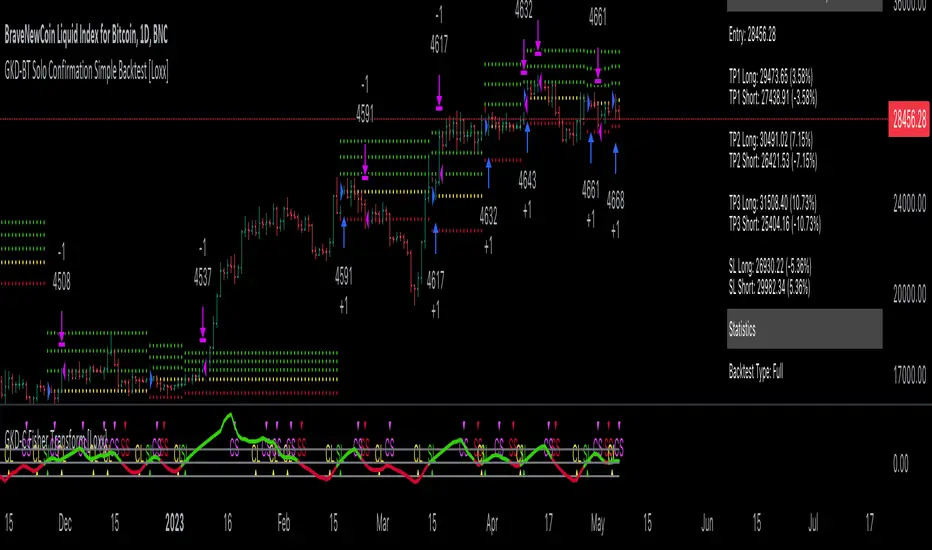
Ruckard TradingLatinoThis strategy tries to mimic TradingLatino strategy.
The current implementation is beta.
Si hablas castellano o espanyol por favor consulta MENSAJE EN CASTELLANO más abajo.
It's aimed at BTCUSDT pair and 4h timeframe.
STRATEGY DEFAULT SETTINGS EXPLANATION
max_bars_back=5000 : This is a random number of bars so that the strategy test lasts for one or two years
calc_on_order_fills=false : To wait for the 4h closing is too much. Try to check if it's worth entering a position after closing one. I finally decided not to recheck if it's worth entering after an order is closed. So it is false.
calc_on_every_tick=false
pyramiding=0 : We only want one entry allowed in the same direction. And we don't want the order to scale by error.
initial_capital=1000 : These are 1000 USDT. By using 1% maximum loss per trade and 7% as a default stop loss by using 1000 USDT at 12000 USDT per BTC price you would entry with around 142 USDT which are converted into: 0.010 BTC . The maximum number of decimal for contracts on this BTCUSDT market is 3 decimals. E.g. the minimum might be: 0.001 BTC . So, this minimal 1000 amount ensures us not to entry with less than 0.001 entries which might have happened when using 100 USDT as an initial capital.
slippage=1 : Binance BTCUSDT mintick is: 0.01. Binance slippage: 0.1 % (Let's assume). TV has an integer slippage. It does not have a percentage based slippage. If we assume a 1000 initial capital, the recommended equity is 142 which at 11996 USDT per BTC price means: 0.011 BTC. The 0.1% slippage of: 0.011 BTC would be: 0.000011 . This is way smaller than the mintick. So our slippage is going to be 1. E.g. 1 (slippage) * 0.01 (mintick)
commission_type=strategy.commission.percent and commission_value=0.1 : According to: binance . com / en / fee / schedule in VIP 0 level both maker and taker fees are: 0.1 %.
BACKGROUND
Jaime Merino is a well known Youtuber focused on crypto trading
His channel TradingLatino
features monday to friday videos where he explains his strategy.
JAIME MERINO STANCE ON BOTS
Jaime Merino stance on bots (taken from memory out of a 2020 June video from him):
'~
You know. They can program you a bot and it might work.
But, there are some special situations that the bot would not be able to handle.
And, I, as a human, I would handle it. And the bot wouldn't do it.
~'
My long term target with this strategy script is add as many
special situations as I can to the script
so that it can match Jaime Merino behaviour even in non normal circumstances.
My alternate target is learn Pine script
and enjoy programming with it.
WARNING
This script might be bigger than other TradingView scripts.
However, please, do not be confused because the current status is beta.
This script has not been tested with real money.
This is NOT an official strategy from Jaime Merino.
This is NOT an official strategy from TradingLatino . net .
HOW IT WORKS
It basically uses ADX slope and LazyBear's Squeeze Momentum Indicator
to make its buy and sell decisions.
Fast paced EMA being bigger than slow paced EMA
(on higher timeframe) advices going long.
Fast paced EMA being smaller than slow paced EMA
(on higher timeframe) advices going short.
It finally add many substrats that TradingLatino uses.
SETTINGS
__ SETTINGS - Basics
____ SETTINGS - Basics - ADX
(ADX) Smoothing {14}
(ADX) DI Length {14}
(ADX) key level {23}
____ SETTINGS - Basics - LazyBear Squeeze Momentum
(SQZMOM) BB Length {20}
(SQZMOM) BB MultFactor {2.0}
(SQZMOM) KC Length {20}
(SQZMOM) KC MultFactor {1.5}
(SQZMOM) Use TrueRange (KC) {True}
____ SETTINGS - Basics - EMAs
(EMAS) EMA10 - Length {10}
(EMAS) EMA10 - Source {close}
(EMAS) EMA55 - Length {55}
(EMAS) EMA55 - Source {close}
____ SETTINGS - Volume Profile
Lowest and highest VPoC from last three days
is used to know if an entry has a support
VPVR of last 100 4h bars
is also taken into account
(VP) Use number of bars (not VP timeframe): Uses 'Number of bars {100}' setting instead of 'Volume Profile timeframe' setting for calculating session VPoC
(VP) Show tick difference from current price {False}: BETA . Might be useful for actions some day.
(VP) Number of bars {100}: If 'Use number of bars (not VP timeframe)' is turned on this setting is used to calculate session VPoC.
(VP) Volume Profile timeframe {1 day}: If 'Use number of bars (not VP timeframe)' is turned off this setting is used to calculate session VPoC.
(VP) Row width multiplier {0.6}: Adjust how the extra Volume Profile bars are shown in the chart.
(VP) Resistances prices number of decimal digits : Round Volume Profile bars label numbers so that they don't have so many decimals.
(VP) Number of bars for bottom VPOC {18}: 18 bars equals 3 days in suggested timeframe of 4 hours. It's used to calculate lowest session VPoC from previous three days. It's also used as a top VPOC for sells.
(VP) Ignore VPOC bottom advice on long {False}: If turned on it ignores bottom VPOC (or top VPOC on sells) when evaluating if a buy entry is worth it.
(VP) Number of bars for VPVR VPOC {100}: Number of bars to calculate the VPVR VPoC. We use 100 as Jaime once used. When the price bounces back to the EMA55 it might just bounce to this VPVR VPoC if its price it's lower than the EMA55 (Sells have inverse algorithm).
____ SETTINGS - ADX Slope
ADX Slope
help us to understand if ADX
has a positive slope, negative slope
or it is rather still.
(ADXSLOPE) ADX cut {23}: If ADX value is greater than this cut (23) then ADX has strength
(ADXSLOPE) ADX minimum steepness entry {45}: ADX slope needs to be 45 degrees to be considered as a positive one.
(ADXSLOPE) ADX minimum steepness exit {45}: ADX slope needs to be -45 degrees to be considered as a negative one.
(ADXSLOPE) ADX steepness periods {3}: In order to avoid false detection the slope is calculated along 3 periods.
____ SETTINGS - Next to EMA55
(NEXTEMA55) EMA10 to EMA55 bounce back percentage {80}: EMA10 might bounce back to EMA55 or maybe to 80% of its complete way to EMA55
(NEXTEMA55) Next to EMA55 percentage {15}: How much next to the EMA55 you need to be to consider it's going to bounce back upwards again.
____ SETTINGS - Stop Loss and Take Profit
You can set a default stop loss or a default take profit.
(STOPTAKE) Stop Loss % {7.0}
(STOPTAKE) Take Profit % {2.0}
____ SETTINGS - Trailing Take Profit
You can customize the default trailing take profit values
(TRAILING) Trailing Take Profit (%) {1.0}: Trailing take profit offset in percentage
(TRAILING) Trailing Take Profit Trigger (%) {2.0}: When 2.0% of benefit is reached then activate the trailing take profit.
____ SETTINGS - MAIN TURN ON/OFF OPTIONS
(EMAS) Ignore advice based on emas {false}.
(EMAS) Ignore advice based on emas (On closing long signal) {False}: Ignore advice based on emas but only when deciding to close a buy entry.
(SQZMOM) Ignore advice based on SQZMOM {false}: Ignores advice based on SQZMOM indicator.
(ADXSLOPE) Ignore advice based on ADX positive slope {false}
(ADXSLOPE) Ignore advice based on ADX cut (23) {true}
(STOPTAKE) Take Profit? {false}: Enables simple Take Profit.
(STOPTAKE) Stop Loss? {True}: Enables simple Stop Loss.
(TRAILING) Enable Trailing Take Profit (%) {True}: Enables Trailing Take Profit.
____ SETTINGS - Strategy mode
(STRAT) Type Strategy: 'Long and Short', 'Long Only' or 'Short Only'. Default: 'Long and Short'.
____ SETTINGS - Risk Management
(RISKM) Risk Management Type: 'Safe', 'Somewhat safe compound' or 'Unsafe compound'. ' Safe ': Calculations are always done with the initial capital (1000) in mind. The maximum losses per trade/day/week/month are taken into account. ' Somewhat safe compound ': Calculations are done with initial capital (1000) or a higher capital if it increases. The maximum losses per trade/day/week/month are taken into account. ' Unsafe compound ': In each order all the current capital is gambled and only the default stop loss per order is taken into account. That means that the maximum losses per trade/day/week/month are not taken into account. Default : 'Somewhat safe compound'.
(RISKM) Maximum loss per trade % {1.0}.
(RISKM) Maximum loss per day % {6.0}.
(RISKM) Maximum loss per week % {8.0}.
(RISKM) Maximum loss per month % {10.0}.
____ SETTINGS - Decimals
(DECIMAL) Maximum number of decimal for contracts {3}: How small (3 decimals means 0.001) an entry position might be in your exchange.
EXTRA 1 - PRICE IS IN RANGE indicator
(PRANGE) Print price is in range {False}: Enable a bottom label that indicates if the price is in range or not.
(PRANGE) Price range periods {5}: How many previous periods are used to calculate the medians
(PRANGE) Price range maximum desviation (%) {0.6} ( > 0 ): Maximum positive desviation for range detection
(PRANGE) Price range minimum desviation (%) {0.6} ( > 0 ): Mininum negative desviation for range detection
EXTRA 2 - SQUEEZE MOMENTUM Desviation indicator
(SQZDIVER) Show degrees {False}: Show degrees of each Squeeze Momentum Divergence lines to the x-axis.
(SQZDIVER) Show desviation labels {False}: Whether to show or not desviation labels for the Squeeze Momentum Divergences.
(SQZDIVER) Show desviation lines {False}: Whether to show or not desviation lines for the Squeeze Momentum Divergences.
EXTRA 3 - VOLUME PROFILE indicator
WARNING: This indicator works not on current bar but on previous bar. So in the worst case it might be VP from 4 hours ago. Don't worry, inside the strategy calculus the correct values are used. It's just that I cannot show the most recent one in the chart.
(VP) Print recent profile {False}: Show Volume Profile indicator
(VP) Avoid label price overlaps {False}: Avoid label prices to overlap on the chart.
EXTRA 4 - ZIGNALY SUPPORT
(ZIG) Zignaly Alert Type {Email}: 'Email', 'Webhook'. ' Email ': Prepare alert_message variable content to be compatible with zignaly expected email content format. ' Webhook ': Prepare alert_message variable content to be compatible with zignaly expected json content format.
EXTRA 5 - DEBUG
(DEBUG) Enable debug on order comments {False}: If set to true it prepares the order message to match the alert_message variable. It makes easier to debug what would have been sent by email or webhook on each of the times an order is triggered.
HOW TO USE THIS STRATEGY
BOT MODE: This is the default setting.
PROPER VOLUME PROFILE VIEWING: Click on this strategy settings. Properties tab. Make sure Recalculate 'each time the order was run' is turned off.
NEWBIE USER: (Check PROPER VOLUME PROFILE VIEWING above!) You might want to turn on the 'Print recent profile {False}' setting. Alternatively you can use my alternate realtime study: 'Resistances and supports based on simplified Volume Profile' but, be aware, it might consume one indicator.
ADVANCED USER 1: Turn on the 'Print price is in range {False}' setting and help us to debug this subindicator. Also help us to figure out how to include this value in the strategy.
ADVANCED USER 2: Turn on the all the (SQZDIVER) settings and help us to figure out how to include this value in the strategy.
ADVANCED USER 3: (Check PROPER VOLUME PROFILE VIEWING above!) Turn on the 'Print recent profile {False}' setting and report any problem with it.
JAIME MERINO: Just use the indicator as it comes by default. It should only show BUY signals, SELL signals and their associated closing signals. From time to time you might want to check 'ADVANCED USER 2' instructions to check that there's actually a divergence. Check also 'ADVANCED USER 1' instructions for your amusement.
EXTRA ADVICE
It's advised that you use this strategy in addition to these two other indicators:
* Squeeze Momentum Indicator
* ADX
so that your chart matches as close as possible to TradingLatino chart.
ZIGNALY INTEGRATION
This strategy supports Zignaly email integration by default. It also supports Zignaly Webhook integration.
ZIGNALY INTEGRATION - Email integration example
What you would write in your alert message:
||{{strategy.order.alert_message}}||key=MYSECRETKEY||
ZIGNALY INTEGRATION - Webhook integration example
What you would write in your alert message:
{ {{strategy.order.alert_message}} , "key" : "MYSECRETKEY" }
CREDITS
I have reused and adapted some code from
'Directional Movement Index + ADX & Keylevel Support' study
which it's from TradingView console user.
I have reused and adapted some code from
'3ema' study
which it's from TradingView hunganhnguyen1193 user.
I have reused and adapted some code from
'Squeeze Momentum Indicator ' study
which it's from TradingView LazyBear user.
I have reused and adapted some code from
'Strategy Tester EMA-SMA-RSI-MACD' study
which it's from TradingView fikira user.
I have reused and adapted some code from
'Support Resistance MTF' study
which it's from TradingView LonesomeTheBlue user.
I have reused and adapted some code from
'TF Segmented Linear Regression' study
which it's from TradingView alexgrover user.
I have reused and adapted some code from
"Poor man's volume profile" study
which it's from TradingView IldarAkhmetgaleev user.
FEEDBACK
Please check the strategy source code for more detailed information
where, among others, I explain all of the substrats
and if they are implemented or not.
Q1. Did I understand wrong any of the Jaime substrats (which I have implemented)?
Q2. The strategy yields quite profit when we should long (EMA10 from 1d timeframe is higher than EMA55 from 1d timeframe.
Why the strategy yields much less profit when we should short (EMA10 from 1d timeframe is lower than EMA55 from 1d timeframe)?
Any idea if you need to do something else rather than just reverse what Jaime does when longing?
FREQUENTLY ASKED QUESTIONS
FAQ1. Why are you giving this strategy for free?
TradingLatino and his fellow enthusiasts taught me this strategy. Now I'm giving back to them.
FAQ2. Seriously! Why are you giving this strategy for free?
I'm confident his strategy might be improved a lot. By keeping it to myself I would avoid other people contributions to improve it.
Now that everyone can contribute this is a win-win.
FAQ3. How can I connect this strategy to my Exchange account?
It seems that you can attach alerts to strategies.
You might want to combine it with a paying account which enable Webhook URLs to work.
I don't know how all of this works right now so I cannot give you advice on it.
You will have to do your own research on this subject. But, be careful. Automating trades, if not done properly,
might end on you automating losses.
FAQ4. I have just found that this strategy by default gives more than 3.97% of 'maximum series of losses'. That's unacceptable according to my risk management policy.
You might want to reduce default stop loss setting from 7% to something like 5% till you are ok with the 'maximum series of losses'.
FAQ5. Where can I learn more about your work on this strategy?
Check the source code. You might find unused strategies. Either because there's not a substantial increases on earnings. Or maybe because they have not been implemented yet.
FAQ6. How much leverage is applied in this strategy?
No leverage.
FAQ7. Any difference with original Jaime Merino strategy?
Most of the times Jaime defines an stop loss at the price entry. That's not the case here. The default stop loss is 7% (but, don't be confused it only means losing 1% of your investment thanks to risk management). There's also a trailing take profit that triggers at 2% profit with a 1% trailing.
FAQ8. Why this strategy return is so small?
The strategy should be improved a lot. And, well, backtesting in this platform is not guaranteed to return theoric results comparable to real-life returns. That's why I'm personally forward testing this strategy to verify it.
MENSAJE EN CASTELLANO
En primer lugar se agradece feedback para mejorar la estrategia.
Si eres un usuario avanzado y quieres colaborar en mejorar el script no dudes en comentar abajo.
Ten en cuenta que aunque toda esta descripción tenga que estar en inglés no es obligatorio que el comentario esté en inglés.
CHISTE - CASTELLANO
¡Pero Jaime!
¡400.000!
¡Tu da mun!
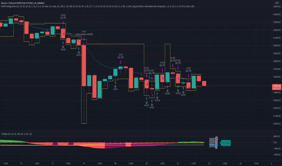
Stochastic Hash Strat [Hash Capital Research]# Stochastic Hash Strategy by Hash Capital Research
## 🎯 What Is This Strategy?
The **Stochastic Slow Strategy** is a momentum-based trading system that identifies oversold and overbought market conditions to capture mean-reversion opportunities. Think of it as a "buy low, sell high" approach with smart mathematical filters that remove emotion from your trading decisions.
Unlike fast-moving indicators that generate excessive noise, this strategy uses **smoothed stochastic oscillators** to identify only the highest-probability setups when momentum truly shifts.
---
## 💡 Why This Strategy Works
Most traders fail because they:
- **Chase prices** after big moves (buying high, selling low)
- **Overtrade** in choppy, directionless markets
- **Exit too early** or hold losses too long
This strategy solves all three problems:
1. **Entry Discipline**: Only trades when the stochastic oscillator crosses in extreme zones (oversold for longs, overbought for shorts)
2. **Cooldown Filter**: Prevents revenge trading by forcing a waiting period after each trade
3. **Fixed Risk/Reward**: Pre-defined stop-loss and take-profit levels ensure consistent risk management
**The Math Behind It**: The stochastic oscillator measures where the current price sits relative to its recent high-low range. When it's below 25, the market is oversold (time to buy). When above 70, it's overbought (time to sell). The crossover with its moving average confirms momentum is shifting.
---
## 📊 Best Markets & Timeframes
### ⭐ OPTIMAL PERFORMANCE:
**Crude Oil (WTI) - 12H Timeframe**
- **Why it works**: Oil markets have predictable volatility patterns and respect technical levels
**AAVE/USD - 4H to 12H Timeframe**
- **Why it works**: DeFi tokens exhibit strong momentum cycles with clear extremes
### ✅ Also Works Well On:
- **BTC/USD** (12H, Daily) - Lower frequency but high win rate
- **ETH/USD** (8H, 12H) - Balanced volatility and liquidity
- **Gold (XAU/USD)** (Daily) - Classic mean-reversion asset
- **EUR/USD** (4H, 8H) - Lower volatility, requires patience
### ❌ Avoid Using On:
- Timeframes below 4H (too much noise)
- Low-liquidity altcoins (wide spreads kill performance)
- Strongly trending markets without pullbacks (Bitcoin in 2021)
- News-driven instruments during major events
---
## 🎛️ Understanding The Settings
### Core Stochastic Parameters
**Stochastic Length (Default: 16)**
- Controls the lookback period for price comparison
- Lower = faster reactions, more signals (10-14 for volatile markets)
- Higher = smoother signals, fewer trades (16-21 for stable markets)
- **Pro tip**: Use 10 for crypto 4H, 16 for commodities 12H
**Overbought Level (Default: 70)**
- Threshold for short entries
- Lower values (65-70) = more trades, earlier entries
- Higher values (75-80) = fewer but higher-conviction trades
- **Sweet spot**: 70 works for most assets
**Oversold Level (Default: 25)**
- Threshold for long entries
- Higher values (25-30) = more trades, earlier entries
- Lower values (15-20) = fewer but stronger bounce setups
- **Sweet spot**: 20-25 depending on market conditions
**Smooth K & Smooth D (Default: 7 & 3)**
- Additional smoothing to filter out whipsaws
- K=7 makes the indicator slower and more reliable
- D=3 is the signal line that confirms the trend
- **Don't change these unless you know what you're doing**
---
### Risk Management
**Stop Loss % (Default: 2.2%)**
- Automatically exits losing trades
- Should be 1.5x to 2x your average market volatility
- Too tight = death by a thousand cuts
- Too wide = uncontrolled losses
- **Calibration**: Check ATR indicator and set SL slightly above it
**Take Profit % (Default: 7%)**
- Automatically exits winning trades
- Should be 2.5x to 3x your stop loss (reward-to-risk ratio)
- This default gives 7% / 2.2% = 3.18:1 R:R
- **The golden rule**: Never have R:R below 2:1
---
### Trade Filters
**Bar Cooldown Filter (Default: ON, 3 bars)**
- **What it does**: Forces you to wait X bars after closing a trade before entering a new one
- **Why it matters**: Prevents emotional revenge trading and overtrading in choppy markets
- **Settings guide**:
- 3 bars = Standard (good for most cases)
- 5-7 bars = Conservative (oil, slow-moving assets)
- 1-2 bars = Aggressive (only for experienced traders)
**Exit on Opposite Extreme (Default: ON)**
- Closes your long when stochastic hits overbought (and vice versa)
- Acts as an early profit-taking mechanism
- **Leave this ON** unless you're testing other exit strategies
**Divergence Filter (Default: OFF)**
- Looks for price/momentum divergences for additional confirmation
- **When to enable**: Trending markets where you want fewer but higher-quality trades
- **Keep OFF for**: Mean-reverting markets (oil, forex, most of the time)
---
## 🚀 Quick Start Guide
### Step 1: Set Up in TradingView
1. Open TradingView and navigate to your chart
2. Click "Pine Editor" at the bottom
3. Copy and paste the strategy code
4. Click "Add to Chart"
5. The strategy will appear in a separate pane below your price chart
### Step 2: Choose Your Market
**If you're trading Crude Oil:**
- Timeframe: 12H
- Keep all default settings
- Watch for signals during London/NY overlap (8am-11am EST)
**If you're trading AAVE or crypto:**
- Timeframe: 4H or 12H
- Consider these adjustments:
- Stochastic Length: 10-14 (faster)
- Oversold: 20 (more aggressive)
- Take Profit: 8-10% (higher targets)
### Step 3: Wait for Your First Signal
**LONG Entry** (Green circle appears):
- Stochastic crosses up below oversold level (25)
- Price likely near recent lows
- System places limit order at take profit and stop loss
**SHORT Entry** (Red circle appears):
- Stochastic crosses down above overbought level (70)
- Price likely near recent highs
- System places limit order at take profit and stop loss
**EXIT** (Orange circle):
- Position closes either at stop, target, or opposite extreme
- Cooldown period begins
### Step 4: Let It Run
The biggest mistake? **Interfering with the system.**
- Don't close trades early because you're scared
- Don't skip signals because you "have a feeling"
- Don't increase position size after a big win
- Don't revenge trade after a loss
**Follow the system or don't use it at all.**
---
### Important Risks:
1. **Drawdown Pain**: You WILL experience losing streaks of 5-7 trades. This is mathematically normal.
2. **Whipsaw Markets**: Choppy, range-bound conditions can trigger multiple small losses.
3. **Gap Risk**: Overnight gaps can cause your actual fill to be worse than the stop loss.
4. **Slippage**: Real execution prices differ from backtested prices (factor in 0.1-0.2% slippage).
---
## 🔧 Optimization Guide
### When to Adjust Settings:
**Market Volatility Increased?**
- Widen stop loss by 0.5-1%
- Increase take profit proportionally
- Consider increasing cooldown to 5-7 bars
**Getting Too Few Signals?**
- Decrease stochastic length to 10-12
- Increase oversold to 30, decrease overbought to 65
- Reduce cooldown to 2 bars
**Getting Too Many Losses?**
- Increase stochastic length to 18-21 (slower, smoother)
- Enable divergence filter
- Increase cooldown to 5+ bars
- Verify you're on the right timeframe
### A/B Testing Method:
1. **Run default settings for 50 trades** on your chosen market
2. Document: Win rate, profit factor, max drawdown, emotional tolerance
3. **Change ONE variable** (e.g., oversold from 25 to 20)
4. Run another 50 trades
5. Compare results
6. Keep the better version
**Never change multiple settings at once** or you won't know what worked.
---
## 📚 Educational Resources
### Key Concepts to Learn:
**Stochastic Oscillator**
- Developed by George Lane in the 1950s
- Measures momentum by comparing closing price to price range
- Formula: %K = (Close - Low) / (High - Low) × 100
- Similar to RSI but more sensitive to price movements
**Mean Reversion vs. Trend Following**
- This is a **mean reversion** strategy (price returns to average)
- Works best in ranging markets with defined support/resistance
- Fails in strong trending markets (2017 Bitcoin, 2020 Tech stocks)
- Complement with trend filters for better results
**Risk:Reward Ratio**
- The cornerstone of profitable trading
- Winning 40% of trades with 3:1 R:R = profitable
- Winning 60% of trades with 1:1 R:R = breakeven (after fees)
- **This strategy aims for 45% win rate with 2.5-3:1 R:R**
### Recommended Reading:
- *"Trading Systems and Methods"* by Perry Kaufman (Chapter on Oscillators)
- *"Mean Reversion Trading Systems"* by Howard Bandy
- *"The New Trading for a Living"* by Dr. Alexander Elder
---
## 🛠️ Troubleshooting
### "I'm not seeing any signals!"
**Check:**
- Is your timeframe 4H or higher?
- Is the stochastic actually reaching extreme levels (check if your asset is stuck in middle range)?
- Is cooldown still active from a previous trade?
- Are you on a low-liquidity pair?
**Solution**: Switch to a more volatile asset or lower the overbought/oversold thresholds.
---
### "The strategy keeps losing money!"
**Check:**
- What's your win rate? (Below 35% is concerning)
- What's your profit factor? (Below 0.8 means serious issues)
- Are you trading during major news events?
- Is the market in a strong trend?
**Solution**:
1. Verify you're using recommended markets/timeframes
2. Increase cooldown period to avoid choppy markets
3. Reduce position size to 5% while you diagnose
4. Consider switching to daily timeframe for less noise
---
### "My stop losses keep getting hit!"
**Check:**
- Is your stop loss tighter than the average ATR?
- Are you trading during high-volatility sessions?
- Is slippage eating into your buffer?
**Solution**:
1. Calculate the 14-period ATR
2. Set stop loss to 1.5x the ATR value
3. Avoid trading right after market open or major news
4. Factor in 0.2% slippage for crypto, 0.1% for oil
---
## 💪 Pro Tips from the Trenches
### Psychological Discipline
**The Three Deadly Sins:**
1. **Skipping signals** - "This one doesn't feel right"
2. **Early exits** - "I'll just take profit here to be safe"
3. **Revenge trading** - "I need to make back that loss NOW"
**The Solution:** Treat your strategy like a business system. Would McDonald's skip making fries because the cashier "doesn't feel like it today"? No. Systems work because of consistency.
---
### Position Management
**Scaling In/Out** (Advanced)
- Enter 50% position at signal
- Add 50% if stochastic reaches 10 (oversold) or 90 (overbought)
- Exit 50% at 1.5x take profit, let the rest run
**This is NOT for beginners.** Master the basic system first.
---
### Market Awareness
**Oil Traders:**
- OPEC meetings = volatility spikes (avoid or widen stops)
- US inventory reports (Wed 10:30am EST) = avoid trading 2 hours before/after
- Summer driving season = different patterns than winter
**Crypto Traders:**
- Monday-Tuesday = typically lower volatility (fewer signals)
- Thursday-Sunday = higher volatility (more signals)
- Avoid trading during exchange maintenance windows
---
## ⚖️ Legal Disclaimer
This trading strategy is provided for **educational purposes only**.
- Past performance does not guarantee future results
- Trading involves substantial risk of loss
- Only trade with capital you can afford to lose
- No one associated with this strategy is a licensed financial advisor
- You are solely responsible for your trading decisions
**By using this strategy, you acknowledge that you understand and accept these risks.**
---
## 🙏 Acknowledgments
Strategy development inspired by:
- George Lane's original Stochastic Oscillator work
- Modern quantitative trading research
- Community feedback from hundreds of backtests
Built with ❤️ for retail traders who want systematic, disciplined approaches to the markets.
---
**Good luck, stay disciplined, and trade the system, not your emotions.**
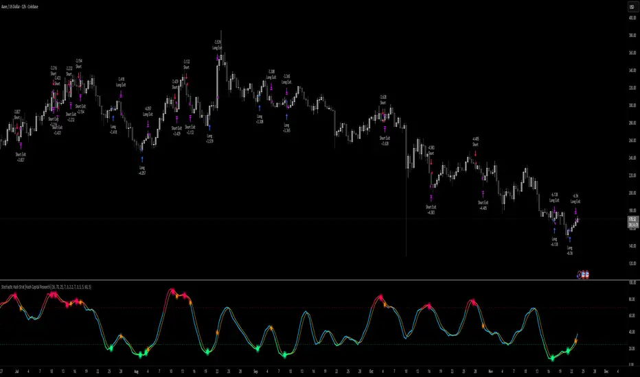
Golden Cross 50/200 EMATrend-following systems are characterized by having a low win rate, yet in the right circumstances (trending markets and higher timeframes) they can deliver returns that even surpass those of systems with a high win rate.
Below, I show you a simple bullish trend-following system with clear execution rules:
System Rules
-Long entries when the 50-period EMA crosses above the 200-period EMA.
-Stop Loss (SL) placed at the lowest low of the 15 candles prior to the entry candle.
-Take Profit (TP) triggered when the 50-period EMA crosses below the 200-period EMA.
Risk Management
-Initial capital: $10,000
-Position size: 10% of capital per trade
-Commissions: 0.1% per trade
Important Note:
In the code, the stop loss is defined using the swing low (15 candles), but the position size is not adjusted based on the distance to the stop loss. In other words, 10% of the equity is risked on each trade, but the actual loss on the trade is not controlled by a maximum fixed percentage of the account — it depends entirely on the stop loss level. This means the loss on a single trade could be significantly higher or lower than 10% of the account equity, depending on volatility.
Implementing leverage or reducing position size based on volatility is something I haven’t been able to include in the code, but it would dramatically improve the system’s performance. It would fix a consistent percentage loss per trade, preventing losses from fluctuating wildly with changes in volatility.
For example, we can maintain a fixed loss percentage when volatility is low by using the following formula:
Leverage = % of SL you’re willing to risk / % volatility from entry point to stop loss
And when volatility is high and would exceed the fixed percentage we want to expose per trade (if the SL is hit), we could reduce the position size accordingly.
Practical example:
Imagine we only want to risk 15% of the position value if the stop loss is triggered on Tesla (which has high volatility), but the distance to the SL represents a potential 23.57% drop. In this case, we subtract the desired risk (15%) from the actual volatility-based loss (23.57%):
23.57% − 15% = 8.57%
Now suppose we normally use $200 per trade.
To calculate 8.57% of $200:
200 × (8.57 / 100) = $17.14
Then subtract that amount from the original position size:
$200 − $17.14 = $182.86
In summary:
If we reduce the position size to $182.86 (instead of the usual $200), even if Tesla moves 23.57% against us and hits the stop loss, we would still only lose approximately 15% of the original $200 position — exactly the risk level we defined. This way, we strictly respect our risk management rules regardless of volatility swings.
I hope this clearly explains the importance of capping losses at a fixed percentage per trade. This keeps risk under control while maintaining a consistent percentage of capital invested per trade — preventing both statistical distortion of the system and the potential destruction of the account.
About the code:
Strategy declaration:
The strategy is named 'Golden Cross 50/200 EMA'.
overlay=true means it will be drawn directly on the price chart.
initial_capital=10000 sets the initial capital to $10,000.
default_qty_type=strategy.percent_of_equity and default_qty_value=10 means each trade uses 10% of available equity.
margin_long=0 indicates no margin is used for long positions (this is likely for simulation purposes only; in real trading, margin would be required).
commission_type=strategy.commission.percent and commission_value=0.1 sets a 0.1% commission per trade.
Indicators:
Calculates two EMAs: a 50-period EMA (ema50) and a 200-period EMA (ema200).
Crossover detection:
bullCross is triggered when the 50-period EMA crosses above the 200-period EMA (Golden Cross).
bearCross is triggered when the 50-period EMA crosses below the 200-period EMA (Death Cross).
Recent swing:
swingLow calculates the lowest low of the previous 15 periods.
Stop Loss:
entryStopLoss is a variable initialized as na (not available) and is updated to the current swingLow value whenever a bullCross occurs.
Entry and exit conditions:
Entry: When a bullCross occurs, the initial stop loss is set to the current swingLow and a long position is opened.
Exit on opposite signal: When a bearCross occurs, the long position is closed.
Exit on stop loss: If the price falls below entryStopLoss while a position is open, the position is closed.
Visualization:
Both EMAs are plotted (50-period in blue, 200-period in red).
Green triangles are plotted below the bar on a bullCross, and red triangles above the bar on a bearCross.
A horizontal orange line is drawn that shows the stop loss level whenever a position is open.
Alerts:
Alerts are created for:Long entry
Exit on bearish crossover (Death Cross)
Exit triggered by stop loss
Favorable Conditions:
Tesla (45-minute timeframe)
June 29, 2010 – November 17, 2025
Total net profit: $12,458.73 or +124.59%
Maximum drawdown: $1,210.40 or 8.29%
Total trades: 107
Winning trades: 27.10% (29/107)
Profit factor: 3.141
Tesla (1-hour timeframe)
June 29, 2010 – November 17, 2025
Total net profit: $7,681.83 or +76.82%
Maximum drawdown: $993.36 or 7.30%
Total trades: 75
Winning trades: 29.33% (22/75)
Profit factor: 3.157
Netflix (45-minute timeframe)
May 23, 2002 – November 17, 2025
Total net profit: $11,380.73 or +113.81%
Maximum drawdown: $699.45 or 5.98%
Total trades: 134
Winning trades: 36.57% (49/134)
Profit factor: 2.885
Netflix (1-hour timeframe)
May 23, 2002 – November 17, 2025
Total net profit: $11,689.05 or +116.89%
Maximum drawdown: $844.55 or 7.24%
Total trades: 107
Winning trades: 37.38% (40/107)
Profit factor: 2.915
Netflix (2-hour timeframe)
May 23, 2002 – November 17, 2025
Total net profit: $12,807.71 or +128.10%
Maximum drawdown: $866.52 or 6.03%
Total trades: 56
Winning trades: 41.07% (23/56)
Profit factor: 3.891
Meta (45-minute timeframe)
May 18, 2012 – November 17, 2025
Total net profit: $2,370.02 or +23.70%
Maximum drawdown: $365.27 or 3.50%
Total trades: 83
Winning trades: 31.33% (26/83)
Profit factor: 2.419
Apple (45-minute timeframe)
January 3, 2000 – November 17, 2025
Total net profit: $8,232.55 or +80.59%
Maximum drawdown: $581.11 or 3.16%
Total trades: 140
Winning trades: 34.29% (48/140)
Profit factor: 3.009
Apple (1-hour timeframe)
January 3, 2000 – November 17, 2025
Total net profit: $9,685.89 or +94.93%
Maximum drawdown: $374.69 or 2.26%
Total trades: 118
Winning trades: 35.59% (42/118)
Profit factor: 3.463
Apple (2-hour timeframe)
January 3, 2000 – November 17, 2025
Total net profit: $8,001.28 or +77.99%
Maximum drawdown: $755.84 or 7.56%
Total trades: 67
Winning trades: 41.79% (28/67)
Profit factor: 3.825
NVDA (15-minute timeframe)
January 3, 2000 – November 17, 2025
Total net profit: $11,828.56 or +118.29%
Maximum drawdown: $1,275.43 or 8.06%
Total trades: 466
Winning trades: 28.11% (131/466)
Profit factor: 2.033
NVDA (30-minute timeframe)
January 3, 2000 – November 17, 2025
Total net profit: $12,203.21 or +122.03%
Maximum drawdown: $1,661.86 or 10.35%
Total trades: 245
Winning trades: 28.98% (71/245)
Profit factor: 2.291
NVDA (45-minute timeframe)
January 3, 2000 – November 17, 2025
Total net profit: $16,793.48 or +167.93%
Maximum drawdown: $1,458.81 or 8.40%
Total trades: 172
Winning trades: 33.14% (57/172)
Profit factor: 2.927

Multi Channel GRID & DCA LTF [trade_lexx]Multi Channel GRID & DCA LTF
Usage Guide
Part 1: The concept and general possibilities of the "Multi Channel GRID & DCA LTF" strategy
Introduction
Welcome to the guide to "Multi Channel GRID & DCA LTF", a powerful and versatile automated trading strategy for the TradingView platform. This tool was developed for traders who are looking for flexibility, control and a high degree of adaptability to various market conditions.
The strategy is based on a hybrid approach that combines two popular and time-tested techniques.:
1. GRID (grid trading): The classic method of averaging a position is by placing a grid of limit orders.
2. DCA (Dollar Cost averaging): Smart position averaging based on signals from external indicators.
However, "Multi Channel GRID & DCA LTF" goes far beyond the simple combination of these two techniques. The strategy includes a number of unique and innovative features, such as cascading MultiGRID grids for dealing with extreme volatility, Channel Mode range trading mode for profiting from sideways movement, and Low Time Frame analysis (LTF) to achieve surgical accuracy in backtesting. Deep customization options for risk management, capital, take profits, and stop losses allow you to configure a strategy for almost any trading style, asset, and timeframe.
The basic idea: How does it work?
Let's take a detailed look at each of the key concepts embedded in the logic of the strategy.
1. GRID — Automatic placement of buy and sell orders at certain price intervals.
This is a fundamental mode of operation. Its main goal is to systematically improve the average entry price for a position if the market is going against you.
* The principle of operation: After opening the base (first) order (`BO`), the strategy automatically places a series of pending limit orders (here they are called "safety orders" or "SO") at certain price intervals. For a long position, orders are placed below the entry price, and for a short position, orders are placed higher.
* Target: When the price moves against an open position, it consistently hits and executes safety orders. Each such execution adds additional volume to the position at a more favorable price, thereby shifting the overall average entry price (`position_avg_price') closer to the current market price. This means that a much smaller corrective movement will be required to gain ground.
* Flexibility: You have full control over the geometry of the grid: the number of safety orders, the percentage distance between them (`SO Step`), and you can even set a coefficient that will increase this step for each subsequent order (`SO Multiplier`), creating an expanding grid.
2. DCA (Signal Averaging) — Smart Averaging
This mode adds an additional layer of analysis to the averaging process. Instead of just buying/selling at the set price levels, the strategy waits for a confirmation signal.
* Working principle: You can connect any external indicator (for example, RSI, CCI, or even your own complex signal system) to the strategy, which outputs numerical values. As standard, 1 is used for a long signal, and -1 is used for a short signal. The strategy will place the next averaging order only at the moment when it receives the appropriate signal.
* Goal: To average a position not just during a fall (or a rise for a short), but at the moments that your main trading system considers the most favorable for this. This allows you to avoid "catching falling knives" and enter only if there are good reasons.
3. Hybrid Mode (GRID+DCA) is the best of the previous two modes
This mode is designed for maximum filtering and control. It requires two conditions to be fulfilled simultaneously.
* Working principle: The safety order will be executed only if the price has reached the calculated grid level and a confirmation signal has been received from your external indicator. If a confirmation signal is received from an external indicator, the next calculated grid level activates the limit order.
* Goal: To create the most reliable averaging system that protects against premature entries and requires double confirmation (both by price and indicator) before increasing the position size.
4. MultiGRID — Adaptation to extreme volatility
This is one of the most powerful and unique features of a strategy designed to survive and make a profit in the face of strong, protracted trends or "black swans".
* The problem it solves: The usual grid of orders has a limited depth. If the price goes beyond the last safety order, the strategy loses the opportunity to average and becomes vulnerable.
* The principle of operation: The MultiGRID function allows you to create "cascades" — several grids following one another. When all the orders of the first grid are executed, the strategy does not stop. Instead, she can activate the second, third (and so on) a grid of orders. The new grid can be activated by one of two triggers:
1. Offset: The new grid is activated when the price passes another set percentage deviation from the last executed order.
2. Signal: The new grid is activated when a signal is received from an external indicator.
* Goal: To significantly expand the working range of the strategy. This allows it to adapt to strong market movements that would "break" the usual grid, and continue to effectively average a position at a much greater depth of decline or growth.
5. Channel Mode — Trading in the range
This feature turns a standard averaging strategy into a machine for "farming" profits within a price channel that is formed during a sideways market movement.
* The problem it solves: In the standard grid strategy, after partially closing a take profit position, the volume of this part "leaves" the trade until the deal is fully closed. You are missing the opportunity to reuse this capital.
* Operating principle: When Channel Mode is enabled, the following happens. Suppose the price went against you, executed several safety orders, and then turned around and reached one of the partial take profits. At this point, the strategy is:
1. Fixes the profit, as it should be.
2. Instantly places a new limit order to buy (or sell for a short) at exactly the same price level where the last triggered safety order was executed. The volume of this order is equal to the volume of the part that was just closed for take profit.
3. If the price goes down again and executes this "repeat" order, the strategy immediately sets a corresponding take profit for it at the level where the previous profit was taken.
* Goal: To create a continuous buy-sell cycle within the local range (channel). The lower limit of the channel is the price of the last averaging, and the upper limit is the price of a partial take profit. This allows you to repeatedly profit from sideways price fluctuations, without waiting for the full closure of the main, large transaction.
6. LTF (Lower Timeframe Analysis) — Surgical precision of backtesting
This feature is critically important for obtaining reliable results during historical testing (backtesting) of grid strategies.
* The problem it solves: The standard testing mechanism in TradingView has a serious limitation. Working, for example, on a 4-hour chart, he sees only 4 candle points: Open, High, Low and Close. He does not know in what order the price moved within these 4 hours. He could have touched High first and then Low, or vice versa. For grid strategies, this is fatal — the engine can show that a take profit has been executed, although in reality the price first went down, collected the entire grid of orders and only then turned around.
* How it works: When you turn on the LTF mode, the strategy for each candle on your main chart (for example, 4H) requests and analyzes all candles from the lower timeframe you specified (for example, 1-minute). Then it virtually trades the entire price path for these minute candles, executing orders, take profits and stop losses in the sequence in which they would occur in reality. It works in the single take profit mode of the Grid strategy.
* Goal: To provide the most realistic and reliable backtest that reflects the real dynamics of the market. This allows you to avoid false expectations and accurately assess the potential performance of the strategy.
// ------------------------
Part 2: Detailed description of the strategy settings
This section is your main guide to all the switches and options available in the strategy. Understanding each setting is the key to unlocking the full potential of this powerful tool.
1. 🛡️ Risk Management 🛡️
This group contains fundamental parameters that determine the basic logic of risk management and the geometry of grid orders.
* Strategy type: Determines the direction of transactions.
* Long: The strategy will only open long positions (buy).
* Short: The strategy will only open short positions (sell).
* Both: The strategy will work both ways, opening long or short depending on the incoming signal.
* SO Count: Sets the maximum number of Safety (averaging) Orders (SO) that the strategy will place within the same grid. If you have MultiGRID enabled, this number applies to each individual grid.
* SO Step (%): This is the base percentage deviation from the entry price at which the first safety order will be placed. For example, at a value of 0.5, the first SO in a long trade will be placed 0.5% lower than the opening price of the base order.
* SO Multiplier: A coefficient that exponentially increases the step for each subsequent safety order. This allows you to create an expanding grid where averaging orders are placed further and further apart, which is effective with strong and accelerating price movements.
* *The step formula for the nth order*: Step(N) = (SO Step) * (SO Multiplier ^(N-1)).
* If the value is 1, all steps will be the same.
* With a value of 1.6, the step of the second SO will be 1.6 times larger than the first, the step of the third will be 1.6 times larger than the second, and so on.
* 1️⃣ TP/SL: These are simplified settings for quick configuration. They allow you to turn on/off the main take profit and stop loss and set basic percentage values for them. More detailed settings for these parameters can be found in the relevant sections below.
// ------------------------
2. 💰 Money Management 💰
Everything related to position size, leverage, and capital is configured here.
* Volume BO (Base Order): Determines the size of the trade's opening order.
* Volume BO: A fixed amount in the quote currency (for example, in USDT).
* USDT (check mark): Manages the information in the comments to the orders. If enabled, the volume of orders in USDT will be displayed in the comments. This is convenient for visual analysis and for sending the amount of USDT by the placeholder {{strategy.order.comment}} via webhooks when connecting the strategy to the exchange or trading terminals.
* or % of deposit: The amount calculated as a percentage of the available capital of the strategy. The check mark to the right of this field enables this mode. Important: using a percentage activates the effect of compounding (compound interest), as the amount of each new transaction will be automatically recalculated based on the current capital (initial capital + profit/loss). If enabled, the percentage of orders will be displayed in the comments. This is convenient for visual analysis and for sending percentages on the placeholder {{strategy.order.comment}} via webhooks when connecting the strategy to the stock exchange, trading terminals, or creating Copy trading.
* Martingale: The coefficient applied to the volume of orders. It increases the size of each subsequent insurance order compared to the base one.
* Volume formula for the nth SO: Volume SO (N) = (Volume BO) * (Martingale^N).
* With a value of 1.2, the volume of the first SO will be 1.2 times greater than the base, the second — 1.44 times (`1.2 * 1.2`) and so on.
* Leverage: Specify the size of your leverage. This parameter is used exclusively for calculating and displaying the approximate liquidation price. It does not affect the size of positions, but it helps to visually assess the risks.
* Liquidation: Enables or disables the calculation and display of the liquidation line on the chart.
* Margin type: Allows you to select a method for calculating the liquidation price, simulating the logic of exchanges:
* Isolated: The liquidation price is calculated based on the size and leverage of the current open position only.
* Cross: The calculation simulates using the entire available balance to maintain a position. In the strategy, the liquidation price is calculated as the level at which the loss on the current transaction is equal to the current capital.
* Commission (%): Specify the percentage of your exchange's commission per transaction. The correct value of this parameter is crucial for obtaining realistic backtest results.
// ------------------------
3. 🕸️ Grid Management 🕸️
This group is responsible for the logic of safety orders and advanced mechanics such as Channel Mode and MultiGRID.
* SO Type: Defines the logic of placing averaging orders.
* GRID: Classic grid. All safety orders are placed in advance as limit orders.
* DCA: Signal averaging. The strategy is waiting for a signal from an external indicator to place a market averaging order.
* GRID+DCA: Hybrid. The strategy waits for a signal, and if it arrives, places a limit order at the appropriate price level of the grid or executes a market order if the signal has arrived below the limit order level.
* Signal for SO: A data source (indicator) that will be used for signals in DCA and GRID+DCA modes.
* ↔️ Channel Mode: When this option is enabled, the strategy tries to trade in a sideways range. After partially closing a take profit position, it immediately places a limit order for re-entry at the price of the last triggered safety order. This creates a buy-sell cycle within the local channel.
* Best Price Only: This filter adds an additional condition for averaging in DCA and MultiGRID modes (when it operates on a signal). The next averaging order or a new grid will be activated only if the current price is more favorable (lower for long, higher for short) than the price of the previous entry.
* 🧩 MultiGRID ⮕ Enables cascading grid mode.
* Grid Count: The total number of grids that can be activated sequentially.
* Offset: Percentage deviation from the price of the last order of the previous grid. When this margin is reached, the following grid of orders is activated (this mode does not require a signal).
* Or signal: Allows you to use the signal from an external indicator as a trigger to activate the next grid. The checkmark on the right turns on this mode.
// ------------------------
4. 🎯 Entry and Stop 🎯
This group of settings allows you to fine-tune the conditions for starting a new trade and all aspects related to protective stop orders, including the complex mechanics of trailing and managing SL after partial take profits.
* 🎯 Signal: A data source (indicator) that will be used to determine when to enter a trade. The strategy expects a value of 1 for the start of a long trade and -1 for a short trade.
* Min Bars: Sets the minimum number of candles that must pass from the moment of opening the previous trade to the moment of opening the next one. A value of 0 disables this filter. This is a useful tool to prevent overly frequent entries in a "noisy" market.
* Non-stop: If this option is enabled, the strategy ignores the Entry Signal and opens a new trade immediately after closing the previous one (taking into account the Min Bars filter, if it is set). This turns the strategy into a constantly working mechanism that is always on the market.
* 🛑 SL Type: Defines the base price from which the stop loss percentage will be calculated. The stop loss in the first section must be enabled for this block of settings to work.
* From the entry point: SL is always calculated from the opening price of the very first base order. It remains static throughout the entire transaction unless it is moved by other functions.
* From breakeven line: SL is dynamically recalculated and shifted each time a safety order is executed. It always follows the average price of the position, being at a given percentage distance from it.
* From last executed SO: SL is recalculated from the price of the last executed order, whether it is a base or a safety order.
* From last SO: SL is calculated from the price of the most recent possible safety order in the grid. This is usually the most remote and conservative type of SL.
* Trailing SL Type: Defines the algorithm by which the stop loss will move after its activation.
* Standard: Classic trailing. After activation, SL will follow the price at a fixed distance.
* ATR: SL will follow the price at a distance equal to the value of the ATR indicator multiplied by the specified multiplier.
* External Source: SL will follow any selected line of the third-party indicator.
* Period and Multiplier: Common parameters for all types of trailing.
* Source: The source of the line for the trailing SL of the third-party indicator.
* Trailing SL after entry: The mode of activation of the trailing SL after entering the transaction
* SL management after TP (sections 1️⃣, 2️⃣, 3️⃣): These three blocks allow you to create a complex stop loss management logic as profits are recorded.
For each take profit level (TP1, TP2, TP3), you can configure:
* SL BE / SL TP1 / SL TP2: When the corresponding TP is reached, the stop loss will be moved to the breakeven point (for TP1), to the TP1 price level (for TP2) or to the TP2 price level (for TP3).
* Trailing SL: When the corresponding TP is reached, the trailing stop loss is activated according to the settings above.
* By ↔️ Signal: A very powerful option. If it is enabled, the above action (SL transfer or trailing activation) will occur when the opposite trading signal is received from an external indicator. This allows you to protect profits or reduce losses if the market turns sharply, even before reaching the target.
* SL Delay ⮕ Allows you to delay the activation of the stop loss.
* Number of Bars: The Stop loss will be physically placed on the market only after the specified number of candles has passed since entering the trade. This can help to avoid "taking out" the stop with a random short movement (squiz) immediately after opening a position.
* SL Block: Unique defensive mechanics for trading both ways (`Strategy Type: Both`).
* Number of SL: If the strategy receives the specified number of stop losses in a row in one direction (for example, 2 stops long), it temporarily blocks the opportunity to open new trades in that direction.
* Lock Reset mode:
* By direction: The lock is lifted if a profitable trade is closed in the allowed direction or if a stop loss is triggered in the opposite direction.
* First profit: The lock is lifted after closing any profitable transaction, regardless of its direction.
// ------------------------
5. ✅ Take Profit ✅
This group of settings provides comprehensive control over profit taking, from a simple take profit to a complex system of partial closures and trailing.
* ✅ TP Type: Defines the base price for calculating the percentage deviation of the take profit.
* From entry point: TP is calculated from the base order price.
* From breakeven line: TP dynamically follows the average position price.
* From last executed SO: TP is calculated from the price of the last executed order.
* Filters for closing on signal
* Only ➕: If TP is triggered by a signal, the deal will be closed only if it is in the black relative to the average price.
* Or >TP: If TP is triggered by a signal, the trade will be closed only if the closing price is better than (or equal to) the estimated price of this TP.
* TP type of trailing: Yes, take profit has a trailing too! It works differently than the SL trailing.
* Standard / ATR: After the price touches the "virtual" TP level, the trailing is activated. He does not place a stop order, but begins to move away from the price, dynamically moving the limit order to close further and further in the profitable direction, allowing him to collect the maximum from the impulse movement.
* External Source: TP will follow any selected line of the third-party indicator.
* Period and Multiplier: Parameters for calculating the trailing margin TP.
* Source: The source of the line for the trailing TP of the third-party indicator.
* TP level settings (sections 1️⃣, 2️⃣, 3️⃣, 4️⃣): The strategy supports up to four independent take profit levels, which allows for a flexible system of partial commits.
For each level, you can set:
* TP: Enable the level and set its percentage deviation from the base price.
* Size: What percentage of the current position will be closed when this level is reached. For the last active TP, this parameter is ignored, and 100% of the remaining position is closed.
* Trailing TP: Enable the above-described trailing mechanism for this particular level.
* Signal: Enable closing based on the signal from the external indicator for this level.
* Or take: If both the closing on the signal and the limit order are enabled, then whatever comes first will work.
* After SO: Activate this TP level only after the specified number of safety orders has been executed. This allows you to set closer targets for riskier (deeply averaged) positions.
// ------------------------
6. 🔬 GRID and MultiGrid Analysis on Lower TFs (LTF) 🔬
This group activates one of the most important functions for accurate testing of grid strategies.
* Enable LTF Calculation ⮕ The main switch of the analysis mode on the lower timeframes.
* Timeframe selection: A drop-down list where you can select a timeframe for detailed analysis. For example, if your main schedule is 1 hour, you can select 1 minute here. The strategy will emulate the trading of minute candles within each hour candle.
❗️Important: As mentioned in the first part, the use of this mode is critically necessary to obtain realistic backtest results, especially for strategies with a dense grid of orders. Without it, the results may be overly optimistic and not reflect the real dynamics of the market. It should be remembered that TradingView imposes a limit on the number of intra-bars (minor TF bars) that can be requested. This is usually about 100,000 bars.
// ------------------------
7. 🕘 Backtest Date Range 🕘
This group allows you to focus testing on a specific historical period.
* Limit Date Range: Enables date filtering.
* Start time: The date and time when the strategy will start analyzing and opening deals.
* End time: The date and time after which the strategy will stop opening new deals and complete testing.
// ------------------------
8. 🎨 Visualization 🎨
All the options responsible for the appearance and information content of the chart are collected here.
* Show PnL labels: Enables/disables the display of text labels with the result (profit/loss) after closing each trade.
* Statistics Table: Enables/disables the main dashboard with detailed statistics on the results of the backtest.
* Strategy Settings Table: Enables/disables an additional panel that summarizes all the key parameters of the current configuration.
* Monthly Profit Table: Enables/disables a table with a breakdown of percentage returns by month and year.
* Table settings: For each of the three tables, you can individually adjust the Text size and Table Position on the screen to position them as conveniently as possible.
* Decimal places: Defines how many decimal places will be displayed in numeric values in tables and on labels.
// ------------------------
9. ✉️ Webhook Settings ✉️
This group is intended for traders who want to automate trading on strategy signals using third-party services and exchanges (for example, 3Commas, WunderTrading, Cryptorobotics, Cryptohopper, Bitsgap, Binance, ByBit, OKX, Pionex, Bitget or proprietary solutions).
For each key event in the strategy, there is a separate switch and a text field:
* Webhook for Open: Enable and set a message for the webhook that will be sent when the base order is opened.
* Webhook for Averaging: A message sent when executing any insurance order.
* Webhook for Take Profit: A message sent when closing on take profit (including partial ones).
* Webhook for Stop-Loss: A message sent when a stop loss is closed.
You can insert a JSON code or any other message format that your service requires for automation into the text fields. The strategy supports special placeholders (for example, `{{strategy.order.alert_message}}`), which allow you to dynamically insert the necessary data into the message, such as the amount of USDT or the percentage of the deposit for entry, averaging and take profit orders.

AccumulationPro Money Flow StrategyAccumulationPro Money Flow Strategy identifies stock trading opportunities by analyzing money flow and potential long-only opportunities following periods of increased money inflow. It employs proprietary responsive indicators and oscillators to gauge the strength and momentum of the inflow relative to previous periods, detecting money inflow, buying/selling pressure, and potential continuation/reversals, while using trailing stop exits to maximize gains while minimizing losses, with careful consideration of risk management and position sizing.
Setup Instructions:
1. Configuring the Strategy Properties:
Click the "Settings" icon (the gear symbol) next to the strategy name.
Navigate to the "Properties" tab within the Settings window.
Initial Capital: This value sets the starting equity for the strategy backtesting. Keep in mind that you will need to specify your current account size in the "Inputs" settings for position sizing.
Base Currency: Leave this setting at its "Default" value.
Order Size: This setting, which determines the capital used for each trade during backtesting, is automatically calculated and updated by the script. You should leave it set to "1 Contract" and the script will calculate the appropriate number of contracts based on your risk per trade, account size, and stop-loss placement.
Pyramiding: Set this setting at 1 order to prevent the strategy from adding to existing positions.
Commission: Enter your broker's commission fee per trade as a percentage, some brokers might offer commission free trading. Verify Price for limit orders: Keep this value as 0 ticks.
Slippage: This value depends on the instrument you are trading, If you are trading liquid stocks on a 1D chart slippage might be neglected. You can Keep this value as 1 ticks if you want to be conservative.
Margin for long positions/short positions: Set both of these to 100% since this strategy does not employ leverage or margin trading.
Recalculate:
Select the "After order is filled" option.
Select the "On every tick" option.
Fill Orders: Keep “Using bar magnifier” unselected.
Select "On bar close". Select "Using standard OHLC"
2. Configuring the Strategy Inputs:
Click the "Inputs" tab in the Settings window.
From/Thru (Date Range): To effectively backtest the strategy, define a substantial period that includes various bullish and bearish cycles. This ensures the testing window captures a range of market conditions and provides an adequate number of trades. It is usually favorable to use a minimum of 8 years for backtesting. Ensure the "Show Date Range" box is checked.
Account Size: This is your actual current Account Size used in the position sizing table calculations.
Risk on Capital %: This setting allows you to specify the percentage of your capital you are willing to risk on each trade. A common value is 0.5%.
3. Configuring Strategy Style:
Select the "Style" tab.
Select the checkbox for “Stop Loss” and “Stop Loss Final” to display the black/red Average True Range Stop Loss step-lines
Make sure the checkboxes for "Upper Channel", "Middle Line", and "Lower Channel" are selected.
Select the "Plots Background" checkboxes for "Color 0" and "Color 1" so that the potential entry and exit zones become color-coded.
Having the checkbox for "Tables" selected allows you to see position sizing and other useful information within the chart.
Have the checkboxes for "Trades on chart" and "Signal Labels" selected for viewing entry and exit point labels and positions.
Uncheck* the "Quantity" checkbox.
Precision: select “Default”.
Check “Labels on price scale”
Check “Values in status line”
Strategy Application Guidelines:
Entry Conditions:
The strategy identifies long entry opportunities based on substantial money inflow, as detected by our proprietary indicators and oscillators. This assessment considers the strength and momentum of the inflow relative to previous periods, in conjunction with strong price momentum (indicated by our modified, less-lagging MACD) and/or a potential price reversal (indicated by our modified, less-noisy Stochastic). Additional confirmation criteria related to price action are also incorporated. Potential entry and exit zones are visually represented by bands on the chart.
A blue upward-pointing arrow, accompanied by the label 'Long' and green band fills, signifies a long entry opportunity. Conversely, a magenta downward-pointing arrow, labeled 'Close entry(s) order Long' with yellow band fills, indicates a potential exit.
Take Profit:
The strategy employs trailing stops, rather than fixed take-profit levels, to maximize gains while minimizing losses. Trailing stops adjust the stop-loss level as the stock price moves in a favorable direction. The strategy utilizes two types of trailing stop mechanisms: one based on the Average True Range (ATR), and another based on price action, which attempts to identify shifts in price momentum.
Stop Loss:
The strategy uses an Average True Range (ATR)-based stop-loss, represented by two lines on the chart. The black line indicates the primary ATR-based stop-loss level, set upon trade entry. The red line represents a secondary ATR stop-loss buffer, used in the position sizing calculation to account for potential slippage or price gaps.
To potentially reduce the risk of stop-hunting, discretionary traders might consider using a market sell order within the final 30 to 60 minutes of the main session, instead of automated stop-loss orders.
Order Types:
Market Orders are intended for use with this strategy, specifically when the candle and signal on the chart stabilize within the final 30 to 60 minutes of the main trading session.
Position Sizing:
A key aspect of this strategy is that its position size is calculated and displayed in a table on the chart. The position size is calculated based on stop-loss placement, including the stop-loss buffer, and the capital at risk per trade which is commonly set around 0.5% Risk on Capital per Trade.
Backtesting:
The backtesting results presented below the chart are for informational purposes only and are not intended to predict future performance. Instead, they serve as a tool for identifying instruments with which the strategy has historically performed well.
It's important to note that the backtester utilizes a tiny portion of the capital for each trade while our strategy relies on a diversified portfolio of multiple stocks or instruments being traded at once.
Important Considerations:
Volume data is crucial; the strategy will not load or function correctly without it. Ensure that your charts include volume data, preferably from a centralized exchange.
Our system is designed for trading a portfolio. Therefore, if you intend to use our system, you should employ appropriate position sizing, without leverage or margin, and seek out a variety of long opportunities, rather than opening a single trade with an excessively large position size.
If you are trading without automated signals, always allow the chart to stabilize. Refrain from taking action until the final 1 hour to 30 minutes before the end of the main trading session to minimize the risk of acting on false signals.
To align with the strategy's design, it's generally preferable to enter a trade during the same session that the signal appears, rather than waiting for a later session.
Disclaimer:
Trading in financial markets involves a substantial degree of risk. You should be aware of the potential for significant financial losses. It is imperative that you trade responsibly and avoid overtrading, as this can amplify losses. Remember that market conditions can change rapidly, and past performance is not indicative of future results. You could lose some or all of your initial investment. It is strongly recommended that you fully understand the risks involved in trading and seek independent financial advice from a qualified professional before using this strategy.

Custom Strategy: ETH Martingale 2.0Strategic characteristics
ETH Little Martin 2.0 is a self-developed trading strategy based on the Martingale strategy, mainly used for trading ETH (Ethereum). The core idea of this strategy is to place orders in the same direction at a fixed price interval, and then use Martin's multiple investment principle to reduce losses, but this is also the main source of losses.
Parameter description:
1 Interval: The minimum spacing for taking profit, stop loss, and opening/closing of orders. Different targets have different spacing. Taking ETH as an example, it is generally recommended to have a spacing of 2% for fluctuations in the target.
2 Base Price: This is the price at which you triggered the first order. Similarly, I am using ETH as an example. If you have other targets, I suggest using the initial value of a price that can be backtesting. The Base Price is only an initial order price and has no impact on subsequent orders.
3 Initial Order Amount: Users can set an initial order amount to control the risk of each transaction. If the stop loss is reached, we will double the amount based on this value. This refers to the value of the position held, not the number of positions held.
4 Loss Multiplier: The strategy will increase the next order amount based on the set multiple after the stop loss, in order to make up for the previous losses through a larger position. Note that after taking profit, it will be reset to 1 times the Initial Order Amount.
5. Long Short Operation: The first order of the strategy is a multiple entry, and in subsequent orders, if the stop loss is reached, a reverse order will be opened. The position value of a one-way order is based on the Loss Multiplier multiple investment, so it is generally recommended that the Loss Multiplier default to 2.
Improvement direction
Although this strategy already has a certain trading logic, there are still some improvement directions that can be considered:
1. Dynamic adjustment of spacing: Currently, the spacing is fixed, and it can be considered to dynamically adjust the spacing based on market volatility to improve the adaptability of the strategy. Try using dynamic spacing, which may be more suitable for the actual market situation.
2. Filtering criteria: Orders and no orders can be optimized separately. The biggest problem with this strategy is that it will result in continuous losses during fluctuations, and eventually increase the investment amount. You can consider filtering out some fluctuations or only focusing on trend trends.
3. Risk management: Add more risk management measures, such as setting a maximum loss limit to avoid huge losses caused by continuous stop loss.
4. Optimize the stop loss multiple: Currently, the stop loss multiple is fixed, and it can be considered to dynamically adjust the multiple according to market conditions to reduce risk.

Donchian Quest Research// =================================
Trend following strategy.
// =================================
Strategy uses two channels. One channel - for opening trades. Second channel - for closing.
Channel is similar to Donchian channel, but uses Close prices (not High/Low). That helps don't react to wicks of volatile candles (“stop hunting”). In most cases openings occur earlier than in Donchian channel. Closings occur only for real breakout.
// =================================
Strategy waits for beginning of trend - when price breakout of channel. Default length of both channels = 50 candles.
Conditions of trading:
- Open Long: If last Close = max Close for 50 closes.
- Close Long: If last Close = min Close for 50 closes.
- Open Short: If last Close = min Close for 50 closes.
- Close Short: If last Close = max Close for 50 closes.
// =================================
Color of lines:
- black - channel for opening trade.
- red - channel for closing trade.
- yellow - entry price.
- fuchsia - stoploss and breakeven.
- vertical green - go Long.
- vertical red - go Short.
- vertical gray - close in end, don't trade anymore.
// =================================
Order size calculated with ATR and volatility.
You can't trade 1 contract in BTC and 1 contract in XRP - for example. They have different price and volatility, so 1 contract BTC not equal 1 contract XRP.
Script uses universal calculation for every market. It is based on:
- Risk - USD sum you ready to loss in one trade. It calculated as percent of Equity.
- ATR indicator - measurement of volatility.
With default setting your stoploss = 0.5 percent of equity:
- If initial capital is 1000 USD and used parameter "Permit stop" - loss will be 5 USD (0.5 % of equity).
- If your Equity rises to 2000 USD and used parameter "Permit stop"- loss will be 10 USD (0.5 % of Equity).
// =================================
This Risk works only if you enable “Permit stop” parameter in Settings.
If this parameter disabled - strategy works as reversal strategy:
⁃ If close Long - channel border works as stoploss and momentarily go Short.
⁃ If close Short - channel border works as stoploss and momentarily go Long.
Channel borders changed dynamically. So sometime your loss will be greater than ‘Risk %’. Sometime - less than ‘Risk %’.
If this parameter enabled - maximum loss always equal to 'Risk %'. This parameter also include breakeven: if profit % = Risk %, then move stoploss to entry price.
// =================================
Like all trend following strategies - it works only in trend conditions. If no trend - slowly bleeding. There is no special additional indicator to filter trend/notrend. You need to trade every signal of strategy.
Strategy gives many losses:
⁃ 30 % of trades will close with profit.
⁃ 70 % of trades will close with loss.
⁃ But profit from 30% will be much greater than loss from 70 %.
Your task - patiently wait for it and don't use risky setting for position sizing.
// =================================
Recommended timeframe - Daily.
// =================================
Trend can vary in lengths. Selecting length of channels determine which trend you will be hunting:
⁃ 20/10 - from several days to several weeks.
⁃ 20/20 or 50/20 - from several weeks to several months.
⁃ 50/50 or 100/50 or 100/100 - from several months to several years.
// =================================
Inputs (Settings):
- Length: length of channel for trade opening/closing. You can choose 20/10, 20/20, 50/20, 50/50, 100/50, 100/100. Default value: 50/50.
- Permit Long / Permit short: Longs are most profitable for this strategy. You can disable Shorts and enable Longs only. Default value: permit all directions.
- Risk % of Equity: for position sizing used Equity percent. Don't use values greater than 5 % - it's risky. Default value: 0.5%.
⁃ ATR multiplier: this multiplier moves stoploss up or down. Big multiplier = small size of order, small profit, stoploss far from entry, low chance of stoploss. Small multiplier = big size of order, big profit, stop near entry, high chance of stoploss. Default value: 2.
- ATR length: number of candles to calculate ATR indicator. It used for order size and stoploss. Default value: 20.
- Close in end - to close active trade in the end (and don't trade anymore) or leave it open. You can see difference in Strategy Tester. Default value: don’t close.
- Permit stop: use stop or go reversal. Default value: without stop, reversal strategy.
// =================================
Properties (Settings):
- Initial capital - 1000 USD.
- Script don't uses 'Order size' - you need to change 'Risk %' in Inputs instead.
- Script don't uses 'Pyramiding'.
- 'Commission' 0.055 % and 'Slippage' 0 - this parameters are for crypto exchanges with perpetual contracts (for example Bybit). If use on other markets - set it accordingly to your exchange parameters.
// =================================
Big dataset used for chart - 'BITCOIN ALL TIME HISTORY INDEX'. It gives enough trades to understand logic of script. It have several good trends.
// =================================
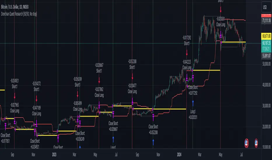
RSI & Backed-Weighted MA StrategyRSI & MA Strategy :
INTRODUCTION :
This strategy is based on two well-known indicators that work best together: the Relative Strength Index (RSI) and the Moving Average (MA). We're going to use the RSI as a trend-follower indicator, rather than a reversal indicator as most are used to. To the signals sent by the RSI, we'll add a condition on the chart's MA, filtering out irrelevant signals and considerably increasing our winning rate. This is a medium/long-term strategy. There's also a money management method enabling us to reinvest part of the profits or reduce the size of orders in the event of substantial losses.
RSI :
The RSI is one of the best-known and most widely used indicators in trading. Its purpose is to warn traders when an asset is overbought or oversold. It was designed to send reversal signals, but we're going to use it as a trend indicator by increasing its length to 20. The RSI formula is as follows :
RSI (n) = 100 - (100 / (1 + (H (n)/L (n))))
With n the length of the RSI, H(n) the average of days closing above the open and L(n) the average of days closing below the open.
MA :
The Moving Average is also widely used in technical analysis, to smooth out variations in an asset. The SMA formula is as follows :
SMA (n) = (P1 + P2 + ... + Pn) / n
where n is the length of the MA.
However, an SMA does not weight any of its terms, which means that the price 10 days ago has the same importance as the price 2 days ago or today's price... That's why in this strategy we use a RWMA, i.e. a back-weighted moving average. It weights old prices more heavily than new ones. This will enable us to limit the impact of short-term variations and focus on the trend that was dominating. The RWMA used weights :
The 4 most recent terms by : 100 / (4+(n-4)*1.30)
The other oldest terms by : weight_4_first_term*1.30
So the older terms are weighted 1.30 more than the more recent ones. The moving average thus traces a trend that accentuates past values and limits the noise of short-term variations.
PARAMETERS :
RSI Length : Lenght of RSI. Default is 20.
MA Type : Choice between a SMA or a RWMA which permits to minimize the impact of short term reversal. Default is RWMA.
MA Length : Length of the selected MA. Default is 19.
RSI Long Signal : Minimum value of RSI to send a LONG signal. Default is 60.
RSI Short signal : Maximum value of RSI to send a SHORT signal. Default is 40.
ROC MA Long Signal : Maximum value of Rate of Change MA to send a LONG signal. Default is 0.
ROC MA Short signal : Minimum value of Rate of Change MA to send a SHORT signal. Default is 0.
TP activation in multiple of ATR : Threshold value to trigger trailing stop Take Profit. This threshold is calculated as multiple of the ATR (Average True Range). Default value is 5 meaning that to trigger the trailing TP the price need to move 5*ATR in the right direction.
Trailing TP in percentage : Percentage value of trailing Take Profit. This Trailing TP follows the profit if it increases, remaining selected percentage below it, but stops if the profit decreases. Default is 3%.
Fixed Ratio : This is the amount of gain or loss at which the order quantity is changed. Default is 400, which means that for each $400 gain or loss, the order size is increased or decreased by a user-selected amount.
Increasing Order Amount : This is the amount to be added to or subtracted from orders when the fixed ratio is reached. The default is $200, which means that for every $400 gain, $200 is reinvested in the strategy. On the other hand, for every $400 loss, the order size is reduced by $200.
Initial capital : $1000
Fees : Interactive Broker fees apply to this strategy. They are set at 0.18% of the trade value.
Slippage : 3 ticks or $0.03 per trade. Corresponds to the latency time between the moment the signal is received and the moment the order is executed by the broker.
Important : A bot has been used to test the different parameters and determine which ones maximize return while limiting drawdown. This strategy is the most optimal on BITSTAMP:ETHUSD with a timeframe set to 6h. Parameters are set as follows :
MA type: RWMA
MA Length: 19
RSI Long Signal: >60
RSI Short Signal : <40
ROC MA Long Signal : <0
ROC MA Short Signal : >0
TP Activation in multiple ATR : 5
Trailing TP in percentage : 3
ENTER RULES :
The principle is very simple:
If the asset is overbought after a bear market, we are LONG.
If the asset is oversold after a bull market, we are SHORT.
We have defined a bear market as follows : Rate of Change (20) RWMA < 0
We have defined a bull market as follows : Rate of Change (20) RWMA > 0
The Rate of Change is calculated using this formula : (RWMA/RWMA(20) - 1)*100
Overbought is defined as follows : RSI > 60
Oversold is defined as follows : RSI < 40
LONG CONDITION :
RSI > 60 and (RWMA/RWMA(20) - 1)*100 < -1
SHORT CONDITION :
RSI < 40 and (RWMA/RWMA(20) - 1)*100 > 1
EXIT RULES FOR WINNING TRADE :
We have a trailing TP allowing us to exit once the price has reached the "TP Activation in multiple ATR" parameter, i.e. 5*ATR by default in the profit direction. TP trailing is triggered at this point, not limiting our gains, and securing our profits at 3% below this trigger threshold.
Remember that the True Range is : maximum(H-L, H-C(1), C-L(1))
with C : Close, H : High, L : Low
The Average True Range is therefore the average of these TRs over a length defined by default in the strategy, i.e. 20.
RISK MANAGEMENT :
This strategy may incur losses. The method for limiting losses is to set a Stop Loss equal to 3*ATR. This means that if the price moves against our position and reaches three times the ATR, we exit with a loss.
Sometimes the ATR can result in a SL set below 10% of the trade value, which is not acceptable. In this case, we set the SL at 10%, limiting losses to a maximum of 10%.
MONEY MANAGEMENT :
The fixed ratio method was used to manage our gains and losses. For each gain of an amount equal to the value of the fixed ratio, we increase the order size by a value defined by the user in the "Increasing order amount" parameter. Similarly, each time we lose an amount equal to the value of the fixed ratio, we decrease the order size by the same user-defined value. This strategy increases both performance and drawdown.
Enjoy the strategy and don't forget to take the trade :)
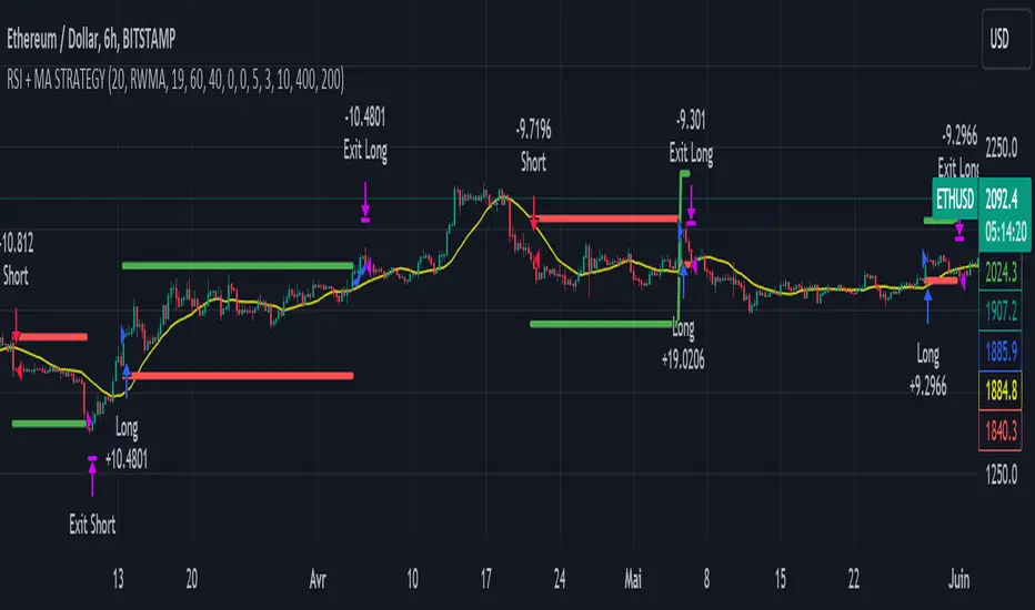
SOFEX Strong Volatility Trend Follower + BacktestingWhat is the SOFEX Strong Volatility Trend Follower + Backtesting script?
🔬 Trading Philosophy
This script is trend-following, attempting to avoid choppy markets.
It has been developed for Bitcoin and Ethereum trading, on 1H timeframe.
The strategy does not aim to make a lot of trades, or to always remain in a position and switch from long to short. Many times there is no direction and the market is in "random walk mode", and chasing trades is futile.
Expectations of performance should be realistic.
The script focuses on a balanced take-profit to stop-loss ratio. In the default set-up of the script, that is a 2% : 2% (1:1) ratio. A relatively low stop loss and take profit build onto the idea that positions should be exited promptly. There are many options to edit these values, including enabling trailing take profit and stop loss. Traders can also completely turn off TP and SL levels, and rely on opposing signals to exit and enter new trades.
Extreme scenarios can happen on the cryptocurrency markets, and disabling stop-loss levels completely is not recommended. The position size should be monitored since all of it is at risk with no stop-loss.
⚙️ Logic of the indicator
The Strong Volatility Trend Follower indicator aims at evading ranging market conditions. It does not seek to chase volatile, yet choppy markets. It aims at aggressively following confirmed trends. The indicator works best during strong, volatile trends, however, it has the downside of entering trades at trend tops or bottoms.
This indicator also leverages proprietary adaptive moving averages to identify and follow strong trend volatility effectively. Furthermore, it uses the Average Directional Index, Awesome Oscillator, ATR and a modified version of VWAP, to categorize trends into weak or strong ones. The VWAP indicator is used to identify the monetary (volume) inflow into a given trend, further helping to avoid short-term manipulations. It also helps to distinguish choppy-market volatility with a trending market one.
📟 Parameters Menu
The script has a comprehensive parameter menu:
Preset Selection : Choose between Bitcoin or Ethereum presets to tailor the indicator to your preferred cryptocurrency market.
Indicator Sensitivity Parameter : Adjust the sensitivity to adapt the indicator, particularly to make it seek higher-strength trends.
Indicator Signal Direction : Set the signal direction as Long, Short, or Both, depending on your preference.
Exit of Signals : You have options regarding Take-Profit (TP) and Stop-Loss (SL) levels. Enable TP/SL levels to exit trades at predetermined levels, or disable them to rely on direction changes for exits. Be aware that removing stop losses can introduce additional risk, and position sizing should be carefully monitored.
By enabling Trailing TP/SL, the system switches to a trailing approach, allowing you to:
- Place an initial customizable SL.
- Specify a level (%) for the Trailing SL to become active.
- When the activation level is reached, the system moves the trailing stop by a given Offset (%).
Additionally, you can enable exit at break-even, where the system places an exit order when the trail activation level is reached, accounting for fees and slippage.
Alert Messages : Define the fields for alert messages based on specific conditions. You can set up alerts to receive email, SMS, and in-app notifications. If you use webhooks for alerts, exercise caution, as these alerts can potentially execute trades without human supervision.
Backtesting : Default backtesting parameters are set to provide realistic backtesting performance:
- 0.04% Commission per trade (for both entries and exits)
- 3 ticks Slippage (highly dependent on exchange)
- Initial capital of $1000
- Order size of $1000
While the order size is equal to the initial capital, the script employs a 2% stop-loss order to limit losses and attempts to prevent risky trades from creating big losses. The order size is a set dollar value, so that the backtesting performance is linear, instead of using % of capital which may result in unrealistic backtesting performance.
Risk Disclaimer
Please be aware that backtesting results, while valuable for statistical overview, do not guarantee future performance in any way. Cryptocurrency markets are inherently volatile and risky. Always trade responsibly and do not risk more than you can afford to lose.
