Globex, Extended, Daily, Weekly, Monthly, Yearly Range* Adds Right Side Only Price Line & Labels for Tracking without Extending Both Sides
* Tracks Current, Previous, and Two Previous Globex Sessions/ Futures:
* Tracks Current, Previous, and Two Previous Extended Session/ Stocks:
* Tracks Current, Previous, Two, & Three Previous Day Session/ Equities:
* Tracks Current, Last, Two, Three, Four, & Five Week Session/ Equities:
* Tracks Current, Last, Two, Three, Four, & Five Month Session/ Equities:
* Tracks Current, Last, Two, Three, Four, & Five Year Session/ Equities:
* Allows Custom Range on Globex, Extended, & Daily Sessions
* Allows Custom Range on Weekly, Monthly, & Yearly Sessions
* Lines & Labels Are Not Visible on Chart Scales
* Reversible Text & Background Color
* Lines Extend Accordingly with Range
* Labels show Price & Percent Change
* Background Colors should match Chart Color to avoid Overlapping Text & Labels
* Lines have Offset Extension
* Labels have Offset Extension
* Globex Session is only visible on Futures & if Current Timeframe is Intraday
* Extended Session is only visible on Stocks & if Current Timeframe is Intraday
* Daily, Weekly, Monthly, & Yearly Sessions are visible on All Symbols & All Timeframes
* Globex, Extended, & Regular use their Default Time Sessions but allow Customization
* For Back Testing Default Sessions, switch over on the Menu to Style and Turn On/Off their Background Color; Any Area on the Chart Without Background Color is Regular Session
"text"に関するスクリプトを検索
Multiple Percentile Ranks (up to 5 sources at a time)This indicator is a visual percentile rank indicator that can display 1 to 5 sources at one time.
The options:
“Sources”
Choose the number of sources you would like to display. The minimum is 1, the maximum is 5.
“Label percent position”
The label for the current percentage of where the source candle ranks.
“Label position”
This displays the source/s you’ve selected, and the chosen bottom rank % and top rank %.
“Label text size”
Displays the text size of all labels.
“Display current % labels”
Switches the labels on/off only for the current percentage rank of each source.
Source options:
ATR: Average True Range
CCI: Commodity Channel Index
COG: Centre of Gravity
Close: closing price
Close Percent: close percentage from previous close
Dollar Value: volume * (high * low * close / 3)
EOM: Ease of Movement: how much volume it takes to move the price in a certain direction
OBV: On-Balance Volume
RANGE: percentage range of the close price
RSI: Relative Strength Index
RVI: Relative Vigor Index
Time Close: if you select the 1 second timeframe it will provide the gap of time between each 1 second close
Volume: each bar’s volume
Volume (MA): volume moving average
Source # where # is the number of the source. Selects the source you’d like.
Ma Length is the number of previous candles to consider when calculating the moving average of the source. Note, the “MA Length” only applies to sources that have the “(MA)” at the end of their name.
Bottom % is the bottom percentage rank of the source you’ve selected. This is a filter to display the candle line graph in red once the percentage rank is equal to the percentage you’ve chosen or below.
Top % is the top percentage rank of the source you’ve selected. This is a filter to display the candle line graph in green once the percentage rank is equal to the percentage you’ve chosen or higher.
A simple example of how to use the indicator:
Select the dropdown menu for source 1 and select volume.
As the candles populate, it will look at previous candles and assign a percentage rank of where the candles are in relation to previous candles.
*Note, the way Tradingview works is it will populate the first candle the chart was active, and continue on. So, let’s say the 3rd candle was the highest volume day. This candle will show up as 100%. If the next day, the 4th candle has an even higher volume, it will show up as 100% also, the previous candles won’t “repaint” to other values and are instead set based on when they were confirmed. So, this indicator works best when there are a lot of previous candles to compare itself to.
To use the bottom % rank filter enter a percentage such as 5%. As it comes across a candle that is 5% or less compared to previous volume candles, then the line graph will shade in red.
The same can be said for the top % rank. So, if you want to see the line graph change to green when it comes across the top 99th percentile rank of volume bars, then set the top % rank to 1% and it will give you extremely high-volume bars in green instead of blue.

Major and Minor Trend Indicator by Nikhil34a V 2.2Title: Major and Minor Trend Indicator by Nikhil34a V 2.2
Description:
The Major and Minor Trend Indicator v2.2 is a comprehensive technical analysis script designed for use with the TradingView platform. This powerful tool is developed in Pine Script version 5 and helps traders identify potential buying and selling opportunities in the stock market.
Features:
SMA Trend Analysis: The script calculates two Simple Moving Averages (SMAs) with user-defined lengths for major and minor trends. It displays these SMAs on the chart, allowing traders to visualize the prevailing trends easily.
Surge Detection: The indicator can detect buying and selling surges based on specific conditions, such as volume, RSI, MACD, and stochastic indicators. Both Buying and Selling surges are marked in black on the chart.
Option Buy Zone Detection: The script identifies the option buy zone based on SMA crossovers, RSI, and MACD values. The buy zone is categorized as "CE Zone" or "PE Zone" and displayed in the table along with the trigger time.
Two-Day High and Low Range: The script calculates the highest high and lowest low of the previous two trading days and plots them on the chart. The area between these points is shaded in semi-transparent green and red colors.
Crossover Analysis: The script analyzes moving average crossovers on multiple timeframes (2-minute, 3-minute, and 5-minute) and displays buy and sell signals accordingly.
Trend Identification: The script identifies the major and minor trends as either bullish or bearish, providing valuable insights into the overall market sentiment.
Usage:
Customize Major and Minor SMA Periods: Adjust the lengths of major and minor SMAs through input parameters to suit your trading preferences.
Enable/Disable Moving Averages: Choose which SMAs to display on the chart by toggling the "showXMA" input options.
Set Surge and Option Buy Zone Thresholds: Modify the surgeThreshold, volumeThreshold, RSIThreshold, and StochThreshold inputs to refine the surge and buy zone detection.
Analyze Crossover Signals: Monitor the crossover signals in the table, categorized by timeframes (2-minute, 3-minute, and 5-minute).
Explore Market Bias and Distance to 2-Day High/Low: The table provides information on market bias, current price movement relative to the previous two-day high and low, and the option buy zone status.
Additional Use Cases:
Surge Indicator:
The script includes a Surge Indicator that detects sudden buying or selling surges in the market. When a buying surge is identified, the "BSurge" label will appear below the corresponding candle with black text on a white background. Similarly, a selling surge will display the "SSurge" label in white text on a black background. These indicators help traders quickly spot strong buying or selling activities that may influence their trading decisions. These surges can be used to identify sudden premium dump zones.
Option Buy Zone:
The Option Buy Zone is an essential feature that identifies potential zones for buying call options (CE Zone) or put options (PE Zone) based on specific technical conditions. The indicator evaluates SMA crossovers, RSI, and MACD values to determine the current market sentiment. When the option buy zone is triggered, the script will display the respective zone ("CE Zone" or "PE Zone") in the table, highlighted with a white background. Additionally, the time when the buy zone was triggered will be shown under the "Option Buy Zone Trigger Time" column.
Price Movement Relative to 2-Day High/Low:
The script calculates the highest high and lowest low of the previous two trading days (high2DaysAgo and low2DaysAgo) and plots these points on the chart. The area between these two points is shaded in semi-transparent green and red colors. The green region indicates the price range between the highpricetoconsider (highest high of the previous two days) and the lower value between highPreviousDay and high2DaysAgo. Similarly, the red region represents the price range between the lowpricetoconsider (lowest low of the previous two days) and the higher value between lowPreviousDay and low2DaysAgo.
Entry Time and Current Zone:
The script identifies potential entry times for trades within the option buy zone. When a valid buy zone trigger occurs, the script calculates the entryTime by adding the durationInMinutes (user-defined) to the startTime. The entryTime will be displayed in the "Entry Time" column of the table. Depending on the comparison between optionbuyzonetriggertime and entryTime, the background color of the entry time will change. If optionbuyzonetriggertime is greater than entryTime, the background color will be yellow, indicating that a new trigger has occurred before the specified duration. Otherwise, the background color will be green, suggesting that the entry time is still within the defined duration.
Current Zone Indicator:
The script further categorizes the current zone as either "CE Zone" (call option zone) or "PE Zone" (put option zone). When the market is trending upwards and the minor SMA is above the major SMA, the currentZone will be set to "CE Zone." Conversely, when the market is trending downwards and the minor SMA is below the major SMA, the currentZone will be "PE Zone." This information is displayed in the "Current Zone" column of the table.
These additional use cases empower traders with valuable insights into market trends, buying and selling surges, option buy zones, and potential entry times. Traders can combine this information with their analysis and risk management strategies to make informed and confident trading decisions.
Note:
The script is optimized for identifying trends and potential trade opportunities. It is crucial to perform additional analysis and risk management before executing any trades based on the provided signals.
Happy Trading!

debugLibrary "debug"
Show Array or Matrix Elements In Table
Use anytime you want to see the elements in an array or a matrix displayed.
Effective debugger, particularly for strategies and complex logic structures.
Look in code to find instructions. Reach out if you need assistance.
Functionality includes:
Viewing the contents of an array or matrix on screen.
Track variables and variable updates using debug()
Track if and when local scopes fire using debugs()
Types Allowed:
string
float
int
string
debug(_col, _row, _name, _value, _msg, _ip)
Debug Variables in Matrix
Parameters:
_col (int) : (int) Assign Column
_row (int) : (int) Assign Row
_name (matrix) : (simple matrix) Matrix Name
_value (string) : (string) Assign variable as a string (str.tostring())
_msg (string)
_ip (int) : (int) (default 1) 1 for continuous updates. 2 for barstate.isnew updates. 3 for barstate.isconfirmed updates. -1 to only add once
Returns: Returns Variable _value output and _msg formatted as '_msg: variableOutput' in designated column and row
debug(_col, _row, _name, _value, _msg, _ip)
Parameters:
_col (int)
_row (int)
_name (matrix)
_value (float)
_msg (string)
_ip (int)
debug(_col, _row, _name, _value, _msg, _ip)
Parameters:
_col (int)
_row (int)
_name (matrix)
_value (int)
_msg (string)
_ip (int)
debug(_col, _row, _name, _value, _msg, _ip)
Parameters:
_col (int)
_row (int)
_name (matrix)
_value (bool)
_msg (string)
_ip (int)
debugs(_col, _row, _name, _msg)
Debug Scope in Matrix - Identify When Scope Is Accessed
Parameters:
_col (int) : (int) Column Number
_row (int) : (int) Row Number
_name (matrix) : (simple matrix) Matrix Name
_msg (string) : (string) Message
Returns: Message appears in debug panel using _col/_row as the identifier
viewArray(_arrayName, _pos, _txtSize, _tRows, s_index, s_border, _rowCol, bCol, _fillCond, _offset)
Array Element Display (Supports float , int , string , and bool )
Parameters:
_arrayName (float ) : ID of Array to be Displayed
_pos (string) : Position for Table
_txtSize (string) : Size of Table Cell Text
_tRows (int) : Number of Rows to Display Data In (columns will be calculated accordingly)
s_index (bool) : (Optional. Default True.) Show/Hide Index Numbers
s_border (bool) : (Optional. Default False.) Show/Hide Border
_rowCol (string)
bCol (color) : = (Optional. Default Black.) Frame/Border Color.
_fillCond (bool) : (Optional) Conditional statement. Function displays array only when true. For instances where size is not immediately known or indices are na. Default = true, indicating array size is set at bar_index 0.
_offset (int) : (Optional) Use to view historical array states. Default = 0, displaying realtime bar.
Returns: A Display of Array Values in a Table
viewArray(_arrayName, _pos, _txtSize, _tRows, s_index, s_border, _rowCol, bCol, _fillCond, _offset)
Parameters:
_arrayName (int )
_pos (string)
_txtSize (string)
_tRows (int)
s_index (bool)
s_border (bool)
_rowCol (string)
bCol (color)
_fillCond (bool)
_offset (int)
viewArray(_arrayName, _pos, _txtSize, _tRows, s_index, s_border, _rowCol, bCol, _fillCond, _offset)
Parameters:
_arrayName (string )
_pos (string)
_txtSize (string)
_tRows (int)
s_index (bool)
s_border (bool)
_rowCol (string)
bCol (color)
_fillCond (bool)
_offset (int)
viewArray(_arrayName, _pos, _txtSize, _tRows, s_index, s_border, _rowCol, bCol, _fillCond, _offset)
Parameters:
_arrayName (bool )
_pos (string)
_txtSize (string)
_tRows (int)
s_index (bool)
s_border (bool)
_rowCol (string)
bCol (color)
_fillCond (bool)
_offset (int)
viewMatrix(_matrixName, _pos, _txtSize, s_index, _resetIdx, s_border, bCol, _fillCond, _offset)
Matrix Element Display (Supports , , , and )
Parameters:
_matrixName (matrix) : ID of Matrix to be Displayed
_pos (string) : Position for Table
_txtSize (string) : Size of Table Cell Text
s_index (bool) : (Optional. Default True.) Show/Hide Index Numbers
_resetIdx (bool)
s_border (bool) : (Optional. Default False.) Show/Hide Border
bCol (color) : = (Optional. Default Black.) Frame/Border Color.
_fillCond (bool) : (Optional) Conditional statement. Function displays matrix only when true. For instances where size is not immediately known or indices are na. Default = true, indicating matrix size is set at bar_index 0.
_offset (int) : (Optional) Use to view historical matrix states. Default = 0, displaying realtime bar.
Returns: A Display of Matrix Values in a Table
viewMatrix(_matrixName, _pos, _txtSize, s_index, _resetIdx, s_border, bCol, _fillCond, _offset)
Parameters:
_matrixName (matrix)
_pos (string)
_txtSize (string)
s_index (bool)
_resetIdx (bool)
s_border (bool)
bCol (color)
_fillCond (bool)
_offset (int)
viewMatrix(_matrixName, _pos, _txtSize, s_index, _resetIdx, s_border, bCol, _fillCond, _offset)
Parameters:
_matrixName (matrix)
_pos (string)
_txtSize (string)
s_index (bool)
_resetIdx (bool)
s_border (bool)
bCol (color)
_fillCond (bool)
_offset (int)
viewMatrix(_matrixName, _pos, _txtSize, s_index, _resetIdx, s_border, bCol, _fillCond, _offset)
Parameters:
_matrixName (matrix)
_pos (string)
_txtSize (string)
s_index (bool)
_resetIdx (bool)
s_border (bool)
bCol (color)
_fillCond (bool)
_offset (int)

Open Interest Chart [LuxAlgo]The Open Interest Chart displays Commitments of Traders %change of futures open interest , with a unique circular plotting technique, inspired from this publication Periodic Ellipses .
🔶 USAGE
Open interest represents the total number of contracts that have been entered by market participants but have not yet been offset or delivered. This can be a direct indicator of market activity/liquidity, with higher open interest indicating a more active market.
Increasing open interest is highlighted in green on the circular plot, indicating money coming into the market, while decreasing open interests highlighted in red indicates money coming out of the market.
You can set up to 6 different Futures Open interest tickers for a quick follow up:
🔶 DETAILS
Circles are drawn, using plot() , with the functions createOuterCircle() (for the largest circle) and createInnerCircle() (for inner circles).
Following snippet will reload the chart, so the circles will remain at the right side of the chart:
if ta.change(chart.left_visible_bar_time ) or
ta.change(chart.right_visible_bar_time)
n := bar_index
Here is a snippet which will draw a 39-bars wide circle that will keep updating its position to the right.
//@version=5
indicator("")
n = bar_index
barsTillEnd = last_bar_index - n
if ta.change(chart.left_visible_bar_time ) or
ta.change(chart.right_visible_bar_time)
n := bar_index
createOuterCircle(radius) =>
var int end = na
var int start = na
var basis = 0.
barsFromNearestEdgeCircle = 0.
barsTillEndFromCircleStart = radius
startCylce = barsTillEnd % barsTillEndFromCircleStart == 0 // start circle
bars = ta.barssince(startCylce)
barsFromNearestEdgeCircle := barsTillEndFromCircleStart -1
basis := math.min(startCylce ? -1 : basis + 1 / barsFromNearestEdgeCircle * 2, 1) // 0 -> 1
shape = math.sqrt(1 - basis * basis)
rad = radius / 2
isOK = barsTillEnd <= barsTillEndFromCircleStart and barsTillEnd > 0
hi = isOK ? (rad + shape * radius) - rad : na
lo = isOK ? (rad - shape * radius) - rad : na
start := barsTillEnd == barsTillEndFromCircleStart ? n -1 : start
end := barsTillEnd == 0 ? start + radius : end
= createOuterCircle(40)
plot(h), plot(l)
🔶 LIMITATIONS
Due to the inability to draw between bars, from time to time, drawings can be slightly off.
Bar-replay can be demanding, since it has to reload on every bar progression. We don't recommend using this script on bar-replay. If you do, please choose the lowest speed and from time to time pause bar-replay for a second. You'll see the script gets reloaded.
🔶 SETTINGS
🔹 TICKERS
Toggle :
• Enabled -> uses the first column with a pre-filled list of Futures Open Interest tickers/symbols
• Disabled -> uses the empty field where you can enter your own ticker/symbol
Pre-filled list : the first column is filled with a list, so you can choose your open interest easily, otherwise you would see COT:088691_F_OI aka Gold Futures Open Interest for example.
If applicable, you will see 3 different COT data:
• COT: Legacy Commitments of Traders report data
• COT2: Disaggregated Commitments of Traders report data
• COT3: Traders in Financial Futures report data
Empty field : When needed, you can pick another ticker/symbol in the empty field at the right and disable the toggle.
Timeframe : Commitments of Traders (COT) data is tallied by the Commodity Futures Trading Commission (CFTC) and is published weekly. Therefore data won't change every day.
Default set TF is Daily
🔹 STYLE
From middle:
• Enabled (default): Drawings start from the middle circle -> towards outer circle is + %change , towards middle of the circle is - %change
• Disabled: Drawings start from the middle POINT of the circle, towards outer circle is + OR -
-> in both options, + %change will be coloured green , - %change will be coloured red .
-> 0 %change will be coloured blue , and when no data is available, this will be coloured gray .
Size circle : options tiny, small, normal, large, huge.
Angle : Only applicable if "From middle" is disabled!
-> sets the angle of the spike:
Show Ticker : Name of ticker, as seen in table, will be added to labels.
Text - fill
• Sets colour for +/- %change
Table
• Sets 2 text colours, size and position
Circles
• Sets the colour of circles, style can be changed in the Style section.
You can make it as crazy as you want:

Correlation TrackerCorrelation Tracker Indicator
The Correlation Tracker indicator calculates and visualizes the correlation between two symbols on a chart. It helps traders and investors understand the relationship and strength of correlation between the selected symbol and another symbol of their choice.
Indicator Features:
- Correlation Calculation: The indicator calculates the correlation between two symbols based on the provided lookback period.
- Correlation Scale: The correlation value is normalized to a scale ranging from 0 to 1 for easy interpretation.
- Table Display: A table is displayed on the chart showing the correlation value and a descriptive label indicating the strength of the correlation.
- Customization Options: Users can customize the text color, table background color, and choose whether to display the Pearson correlation value.
- The Correlation Tracker indicator utilizes a logarithmic scale calculation, making it particularly suitable for longer timeframes such as weekly charts, thereby providing a more accurate and balanced measure of correlations across a wide range of values.
How to Use:
1. Select the symbol for which you want to track the correlation (default symbol is "SPX").
2. Adjust the lookback period to define the historical data range for correlation calculation.
3. Customize the text color and table background color according to your preference.
4. Choose whether to display the Pearson correlation value or a descriptive label for correlation strength.
5. Observe the correlation line on the chart, which changes color based on the strength of the correlation.
6. Refer to the correlation table for the exact correlation value or the descriptive label indicating the correlation strength.
Note: The indicator can be applied to any time frame chart and is not limited to logarithmic scale.

Mad_StandardpartsLibrary "Mad_Standardparts"
This are my Standardparts used in upcoming scipts
roundTo(_value, _decimals)
Round a floating point value to a specified number of decimal places.
@description This function takes a floating point value and rounds it to a specified number of decimal places.
Parameters:
_value (float) : The floating point value to be rounded.
_decimals (int) : The number of decimal places to round to. Must be a non-negative integer.
Returns: The rounded value, as a floating point number.
clear_all()
Delete all drawings on the chart.
@description This function deletes all drawings on the chart, including lines, boxes, and labels.
Returns: None.
shifting(_value)
Create a string of spaces to shift text over by a specified amount.
@description This function takes an integer value and returns a string consisting of that many spaces, which can be used to shift text over in a PineScript chart.
Parameters:
_value (int) : The number of spaces to create in the output string.
Returns: A string consisting of the specified number of spaces.
fromLog(_value)
Convert a linear value to a logarithmic value.
@description This function takes a linear value and converts it to a logarithmic value, using the formula specified in the code.
Parameters:
_value (float)
Returns: The corresponding logarithmic value, as a floating point number.
toLog(_value)
Convert a logarithmic value to a linear value.
@description This function takes a logarithmic value and converts it to a linear value, using the formula specified in the code.
Parameters:
_value (float)
Returns: The corresponding linear value, as a floating point number.
f_getbartime()
Calculate the time per bar on the chart.
@description This function calculates the time per bar on the chart based on the first 100 bars.
Returns: The time per bar, as an integer value.

SuperTrend with Chebyshev FilterModified Super Trend with Chebyshev Filter
The Modified Super Trend is an innovative take on the classic Super Trend indicator. This advanced version incorporates a Chebyshev filter, which significantly enhances its capabilities by reducing false signals and improving overall signal quality. In this post, we'll dive deep into the Modified Super Trend, exploring its history, the benefits of the Chebyshev filter, and how it effectively addresses the challenges associated with smoothing, delay, and noise.
History of the Super Trend
The Super Trend indicator, developed by Olivier Seban, has been a popular tool among traders since its inception. It helps traders identify market trends and potential entry and exit points. The Super Trend uses average true range (ATR) and a multiplier to create a volatility-based trailing stop, providing traders with a dynamic tool that adapts to changing market conditions. However, the original Super Trend has its limitations, such as the tendency to produce false signals during periods of low volatility or sideways trading.
The Chebyshev Filter
The Chebyshev filter is a powerful mathematical tool that makes an excellent addition to the Super Trend indicator. It effectively addresses the issues of smoothing, delay, and noise associated with traditional moving averages. Chebyshev filters are named after Pafnuty Chebyshev, a renowned Russian mathematician who made significant contributions to the field of approximation theory.
The Chebyshev filter is capable of producing smoother, more responsive moving averages without introducing additional lag. This is possible because the filter minimizes the worst-case error between the ideal and the actual frequency response. There are two types of Chebyshev filters: Type I and Type II. Type I Chebyshev filters are designed to have an equiripple response in the passband, while Type II Chebyshev filters have an equiripple response in the stopband. The Modified Super Trend allows users to choose between these two types based on their preferences.
Overcoming the Challenges
The Modified Super Trend addresses several challenges associated with the original Super Trend:
Smoothing: The Chebyshev filter produces a smoother moving average without introducing additional lag. This feature is particularly beneficial during periods of low volatility or sideways trading, as it reduces the number of false signals.
Delay: The Chebyshev filter helps minimize the delay between price action and the generated signal, allowing traders to make timely decisions based on more accurate information.
Noise Reduction: The Chebyshev filter's ability to minimize the worst-case error between the ideal and actual frequency response reduces the impact of noise on the generated signals. This feature is especially useful when using the true range as an offset for the price, as it helps generate more reliable signals within a reasonable time frame.
The Great Replacement
The Modified Super Trend with Chebyshev filter is an excellent replacement for the original Super Trend indicator. It offers significant improvements in terms of signal quality, responsiveness, and accuracy. By incorporating the Chebyshev filter, the Modified Super Trend effectively reduces the number of false signals during low volatility or sideways trading, making it a more reliable tool for identifying market trends and potential entry and exit points.
In-Depth Guide to the Modified Super Trend Settings
The Modified Super Trend with Chebyshev filter offers a wide range of settings that allow traders to fine-tune the indicator to suit their specific trading styles and objectives. In this section, we will discuss each setting in detail, explaining its purpose and how to use it effectively.
Source
The source setting determines the price data used for calculations. The default setting is hl2, which calculates the average of the high and low prices. You can choose other price data sources such as close, open, or ohlc4 (average of open, high, low, and close prices) based on your preference.
Up Color and Down Color
These settings control the color of the trend line when the market is in an uptrend (up_color) and a downtrend (down_color). You can customize these colors to your liking, making it easier to visually identify the current market trend.
Text Color
This setting controls the color of the text displayed on the chart when using labels to indicate trend changes. You can choose any color that contrasts well with your chart background for better readability.
Mean Length
The mean_length setting determines the length (number of bars) used for the Chebyshev moving average calculation. A shorter length will make the moving average more responsive to price changes, while a longer length will produce a smoother moving average. It is crucial to find the right balance between responsiveness and smoothness, as a too-short length may generate false signals, while a too-long length might produce lagging signals. The default value is 64, but you can experiment with different values to find the optimal setting for your trading strategy.
Mean Ripple
The mean_ripple setting influences the Chebyshev filter's ripple effect in the passband (Type I) or stopband (Type II). The ripple effect represents small oscillations in the frequency response, which can impact the moving average's smoothness. The default value is 0.01, but you can experiment with different values to find the best balance between smoothness and responsiveness.
Chebyshev Type: Type I or Type II
The style setting allows you to choose between Type I and Type II Chebyshev filters. Type I filters have an equiripple response in the passband, while Type II filters have an equiripple response in the stopband. Depending on your preference for smoothness and responsiveness, you can choose the type that best fits your trading style.
ATR Style
The atr_style setting determines the method used for calculating the Average True Range (ATR). By default (false), it uses the traditional high-low range. When set to true, it uses the absolute difference between the open and close prices. You can choose the method that works best for your trading strategy and the market you are trading.
ATR Length
The atr_length setting controls the length (number of bars) used for calculating the ATR. Similar to the mean_length, a shorter length will make the ATR more responsive to price changes, while a longer length will produce a smoother ATR. The default value is 64, but you can experiment with different values to find the optimal setting for your trading strategy.
ATR Ripple
The atr_ripple setting, like the mean_ripple, influences the ripple effect of the Chebyshev filter used in the ATR calculation. The default value is 0.05, but you can experiment with different values to find the best balance between smoothness and responsiveness.
Multiplier
The multiplier setting determines the factor by which the ATR is multiplied before being added
Super Trend Logic and Signal Optimization
The Modified Super Trend with Chebyshev filter is designed to minimize false signals and provide a clear indication of market trends. It does so by using a combination of moving averages, Average True Range (ATR), and a multiplier. In this section, we will discuss the Super Trend's logic, its ability to prevent false signals, and the early warning crosses added to the indicator.
Super Trend Logic
The Super Trend's logic is based on a combination of the Chebyshev moving average and ATR. The Chebyshev moving average is a smooth moving average that effectively filters out market noise, while the ATR is a measure of market volatility.
The Super Trend is calculated by adding or subtracting a multiple of the ATR from the Chebyshev moving average. The multiplier is a user-defined value that determines the distance between the trend line and the price action. A larger multiplier results in a wider channel, reducing the likelihood of false signals but potentially missing out on valid trend changes.
Preventing False Signals
The Super Trend is designed to minimize false signals by maintaining its trend direction until a significant change in the market occurs. In a downtrend, the trend line will only decrease in value, and in an uptrend, it will only increase. This helps prevent false signals caused by temporary price fluctuations or market noise.
When the price crosses the trend line, the Super Trend does not immediately change its direction. Instead, it employs a safety logic to ensure that the trend change is genuine. The safety logic checks if the new trend line (calculated using the updated moving average and ATR) is more extreme than the previous one. If it is, the trend line is updated; otherwise, the previous trend line is maintained. This mechanism further reduces the likelihood of false signals by ensuring that the trend line only changes when there is a significant shift in the market.
Early Warning Crosses
To provide traders with additional insight, the Modified Super Trend with Chebyshev filter includes early warning crosses. These crosses are plotted on the chart when the price crosses the trend line without the safety logic. Although these crosses do not necessarily indicate a trend change, they can serve as a valuable heads-up for traders to monitor the market closely and prepare for potential trend reversals.
In conclusion, the Modified Super Trend with Chebyshev filter offers a significant improvement over the original Super Trend indicator. By incorporating the Chebyshev filter, this modified version effectively addresses the challenges of smoothing, delay, and noise reduction while minimizing false signals. The wide range of customizable settings allows traders to tailor the indicator to their specific needs, while the inclusion of early warning crosses provides valuable insight into potential trend reversals.
Ultimately, the Modified Super Trend with Chebyshev filter is an excellent tool for traders looking to enhance their trend identification and decision-making abilities. With its advanced features, this indicator can help traders navigate volatile markets with confidence, making more informed decisions based on accurate, timely information.

Sushi Trend [HG]🍣 The Sushi Roll, a trading concept conceived at a restaurant by Mark Fisher.
While the indicator itself goes by Sushi Trend, it is completely backed by the idea of Mark Fisher's Sushi Roll Reversal Pattern. No, it has nothing to do with raw fish, it just so happens that somebody was ordering sushi during the discussion of the idea, and that's how it got its name.
📝 Origin
First mentioned in his book, The Logical Trader --- the idea of the Sushi Roll is to serve as an early warning system to identify reversals in the market. Fisher defines the pattern as a series of 10 bars, split into two different sections, seen as 5 and 5. In order for the pattern to be emitted, the 5 bars to the right must completely engulf the 5 bars to the left. It's not a super complex system and is in fact extremely simple to grasp.
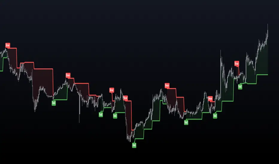
📈 Supertrend Similarities
Instead of displaying the pattern in the way Fisher meant for it to be portrayed (as seen in the photo above), I instead turned it into an indicator similar to that of Supertrend while also inheriting the same concepts from the pattern. I did this because the pattern itself has inconsistencies which can be quite noticeable when trading with it after a while. For example, these patterns can occur even during consolidating periods, and even though the pattern is meant to be recognized during trending markets, the engulfing bars can sometimes be left with indecisive directions.
➡️ The Result
Here is the result, visualized to be better in a trending format. (The indicator will not contain the boxes.)
While Fisher does mention the pattern to include 10 bars, you can actually use this pattern with any number of bars. At the end of the day, it's a concept derived from a discussion at a Japanese restaurant, and a pattern that has been around for years that has seen results. Due to this, I added an input option to control the series of bars for right-bar engulf detection.
To reassure the meaning of the pattern --> "A series of 10 bars" means 5 left bars and 5 right bars. So if you want to check if 5 right bars are engulfing the previous 5 bars (as seen in the photo above), you would want to select 5 in the input settings.
You can learn more about it from the following links
Market Reversals and the Sushi Roll Technique
The Logical Trader
Forex Sessions by CryptoforForex Sessions Boxes
Killzones are the period of greatest volatility, and volatility is one of the main factors for finding the optimal trade time (OTT/Optimal Trade Time). That is, in a period of high volatility, we as traders have the most chances to open a good position, and at the same time not to sit on the charts for too long waiting for its closing.
Sessions:
1. Asian Session:
2. Frankfurt Session:
3. London Session:
3. New York Session:
Features:
Time zone change
Session time change
Show/hide Historical Data
Show/hide Pips
Show/hide Previous Day High/Low
Show/hide New York Midnight/True Daily Open
Text size and align customization
Borders style
Line and border sizes
Full customization of colors: borders, price lines, text, background
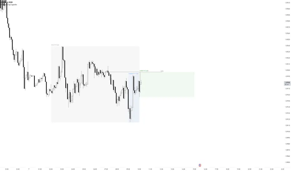
Statistics: High & Low timings of custom session; 1yr historyGet statistics of the Session High and Session Low timings for any custom session; based on around 1yr of data.
//Purpose:
-To get data on the 'time of day' tendencies of an asset.
-Narrow in on a custom defined session and get statistics on that session.
//Notes:
-Input times are always in New York time (but changing the timezone after setting WILL adust both table stats and background highlight correctly.
-For particularly long sessions, make sure text size is set to 'tiny' (very long vertical table), or adjust table to display horizontally.
-You'll notice most assets show higher readings around NY equities open (9:30am NY time). Other assets will have 'hot-spots' at other times too.
-Timings represent the beginning of a 15m candle. i.e. reading for 15:45 represents a high occurring between 15:45 and 1600.
-Premium users should get 20k bars => around 1year's worth of data on a 15minute chart. Days of history is displayed in the top left corner of the table.
//Limitations
-only designed and working on 15minute timeframe (to gather a full year of meaningful/comparable % stats, need 15minute 'buckets' of time.
-sessions cannot cross through midnight, or start at midnight (00:15 is ok). 00:15 >> 23:45 is the max session length. On BTC, same applies but 01:00 instead of midnight (all in NY time).
-if your session crosses through 'dead time' (e.g. 17:00-18:00 S&P NY time); table will correctly omit these non-existent candles, but it will add on the missing hour before the start time.
//Cautionary note:
-Since markets are not uncommonly in a trending state when your defined session starts or ends, the high/low timings % readings for start and end of session may be misleadingly high. Try to look for unusually high readings that are not at the start/end of your session.
Wheat (ZW1!) 15min chart; Table displayed vertically:
Nasdaq (NQ1!) 15m chart; Table displayed horizontally and with smaller text to view a very long custom session:

Pivot Highs&lows: Short/Medium/Long-term + Spikeyness FilterShows Pivot Highs & Lows defined or 'Graded' on a fractal basis: Short-term, medium-term and long-term. Also applies 'Spikeyness' condition by default to filter-out weak/rounded pivots
ES1! 4hr chart (CME) shown above, with lookback = 15; clearly identifying the major highs & lows on the basis of how they are fractally 'nested' within lesser Pivots.
-- in the above chart Short term pivot highs (STH) are simply represented by green 'ʌ', and short-term pivot lows (STL) are simply represented by orange 'v'.
//Basics: (as applying to pivot highs, the following is reversed for pivot lows)
-Short term highs (STH) are simple pivot highs, albeit refined from standard with the 'spikeyness' filter.
-Medium-term highs (MTH) are defined as having a lower STH on either side of them.
-Long-term highs (LTH) are defined as having a lower MTH on either side of them.
//Purpose:
-Education: Quick and easy visualization of the strength or importance of a pivot high or low; a way of grading them based on their larger context.
-Backtesting: use in combination with other trading methods when backtesting to see the relative significance and price sensitivity of LTHs/LTLs compared to lower grade highs and lows.
//Settings:
-Choose Pivot lookback/lookforward bars: One setting, the basis from which all further pivot calculations are done.
-Toggle on/off 'Spikeyness' condition to filter-out weak/rounded/unimpressive pivot highs or lows (default is ON).
-Toggle on/off each of STH, MTH, LTH, STL, MTL, LTL; and choose label text-styles/colors/sizes independently.
-Set text Vertically, horizonally, or simply use 'ʌ' or 'v' symbols if you want to declutter your chart.
//Usage notes:
-Pivots take time to print (lookback bars must have elapsed before confirmation). Fractally nested pivots as here (i.e. a LTH), take even longer to print/confirm, so please be patient.
-Works across timeframes & Assets. Different timeframes may require slightly tweaked lookback/forward settings for optimal use; default is 15 bars.
Example usage with just symbolic labels short-term, med-term, long-term with 1x, 2x and 3x ʌ/v respectively:

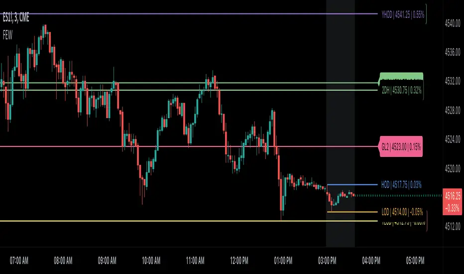
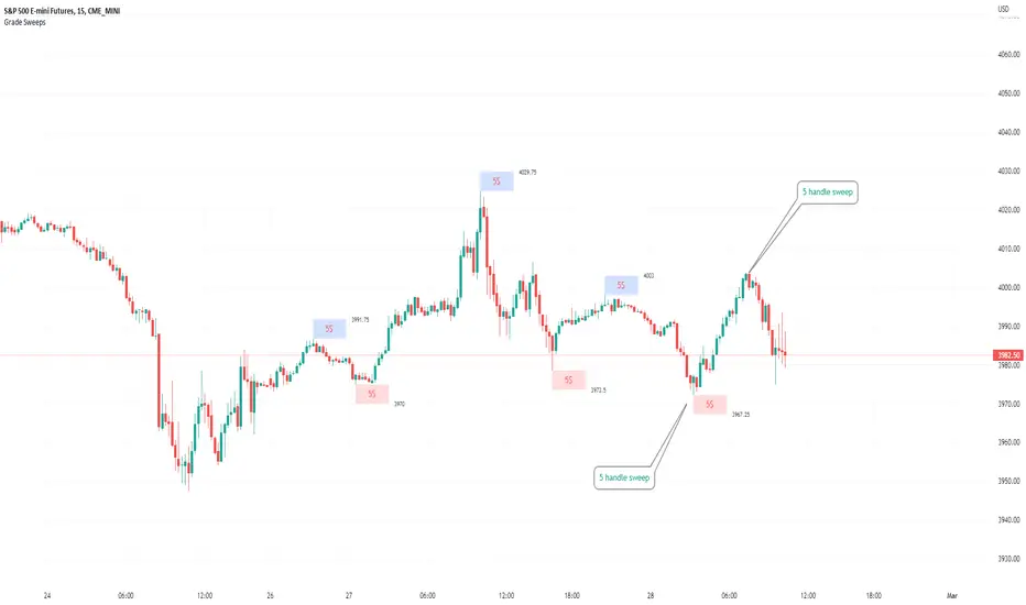
Typical Sweeps: Pivot high/low boxes. Grade sweeps, Handles/PipsTool to show typical pip-grade/ handle-grade sweep distance above pivot highs and pivot lows
-In consolidation/ranging periods (i.e. most of the time); Highs/Lows may by swept by fairly consistent distances in typical stop raids.
-Idea is from ICT teaching on typical Pip-grade sweeps in FX (10,20,30pips). Designed to work on FX, Indices, Commodities, Bitcoin.
-Above chart shows S&P; sweeping below and then above by 5 handles.
///inputs///
~choose sweep distance handles ($) or pips: will auto-calculate depending on the asset: FX= pips; Indices/stocks/commodities = handles ($)
--(2,5,10,20,30,50,100, 500, 1000)
~choose pivot lookback: larger number for more significant swing highs/lows
~choose number of historical boxes to display
~toggle on/off Pivot high boxes and Pivot low boxes independently
~extend boxes fully to the right (default is not extend)
~toggle on/off text
~text & box formatting options
Bitcoin, hourly chart; Pivot lookback = 15; $100 sweep boxes:
Eur/Usd; 15m chart; Pivot lookback = 30; 10pip sweep boxes; Boxes extended fully to the right:
Peer Performance - NIFTY36STOCKSI have created a peer performance dashboard for:
36 stocks from:
5 sectors of Nifty 100
This kind of dashboard is very useful for traders when they are planing to trade in a stocks and like to see how that is stocks is performing against other stocks in the same sector . Picking outperforming stocks will always give outstanding results when market starts moving. os having view on teh complete sector will always be good for traders before picking a specific stock.
Sectors covered in this indicators are:
Indian Auto Sector
Banking Sector
Oil, Gas and Energy Stocks
Cement Sector
Technology Sector
It will help traders reviewing performance ( stock return in last 1 year) of group of stocks from a particular sector .
Basically 5 functions are used to plot this dashboard
using "if " function to shortlist the stocks and the sector it belongs to.
tablo function to plot a table with specific parameters like number of row and columns, color of the frame of table
Getting yearly return into a series of variables using "request.security" function
str.tostring function is used to convert yearly return into a series of text so that it can inserted into the table cell.
finally plotting all the text and yearly return values using table.cell function

Bodies X Wix Version of Smart Money Tools by makuchaku & eFeThis is the same Script as Super Fair Value Gaps / FVG /BoS / by makuchaku & eFe. Mine Should Default to Large Text instead of small. The Super Order Blocks I believe was meant to for you to find one of the many Smart Money tools such as turn on the Fair Value gap but leave the others off, or Turn on where the Break of Structure and leave the others off. The reason I believe this is because the default values for each of the structures were default colored (green for positive and red for negative) for all.
Mine has a different Color for every possible structure. As long as you can read with the larger text that I added, then you can create your own boxes positive for break of structure, rejection block, order blocks and fair value gaps for any time frame. The reason I did that is because There's only certain things I believe I will need to mark for myself in each time frame, and then from there You can stretch iyour own box out further in time because if price touches a fair value gap for example, the fair value gap should conyinue in time until at least 2 candles have filed the Fair valu gap going both directions. That's truly when the fair value gap should is mitigated and will from off the chart. However, If I knew How to add the code for that, I would.
Additionally, I have the Max Boxes per chart, so you should have the ability to see every OB, FVG,RJB, & BoS on the chart
I tried my hardest to create a colored border that was different from the box. But the way the original was coded was almost impossible to do. Because they defined each of the structures (FVG, OB, BoS, RJB) outer levels, when the outer levels connect via math in the code, then it joins all the outside lines for a rectangle. When creating a box, the coloe will always be the same as the border unfortunately. (Unless I replan this from the beginning)
I also Changed the default labels for reach structure from a hard to read gray to a white that pops out.
Also, chart indicators are a little large as well. Such as the cross, sideways cross, The green Triangle, and the white Diamond. You'll get used to it or you can change it as well.
Creating videos for students, you need something they can see.
So, I just wanted to ensure everything was a little more unique and easily usable when showing this to my students when I send them private videos for our weekly lessons. I'm trying to learn how to use the IPFS for THAT, (which i see has invaded PineScript) Hope this indicator helps.
If you're to borrow this, Just make sure you keep the authors in the name makuchaku & efe

ahpuhelperLibrary "ahpuhelper"
Helper Library for Auto Harmonic Patterns UltimateX. It is not meaningful for others. This is supposed to be private library. But, publishing it to make sure that I don't delete accidentally. Some functions may be useful for coders.
insert_open_trades_table_column(showOpenTrades, table_id, column, colors, values, intStatus, harmonicTrailingStartState, lblSizeOpenTrades)
add data to open trades table column
Parameters:
showOpenTrades : flag to show open trades table
table_id : Table Id
column : refers to pattern data
colors : backgroud and text color array
values : cell values
intStatus : status as integer
harmonicTrailingStartState : trailing Start state as per configs
lblSizeOpenTrades : text size
Returns: nextColumn
populate_closed_stats(ClosedStatsPosition, bullishCounts, bearishCounts, bullishRetouchCounts, bearishRetouchCounts, bullishSizeMatrix, bearishSizeMatrix, bullishRR, bearishRR, allPatternLabels, flags, rowMain, rowHeaders)
populate closed stats for harmonic patterns
Parameters:
ClosedStatsPosition : Table position for closed stats
bullishCounts : Matrix containing bullish trade stats
bearishCounts : Matrix containing bearish trade stats
bullishRetouchCounts : Matrix containing bullish trade stats for those which retouched entry
bearishRetouchCounts : Matrix containing bearish trade stats for those which retouched entry
bullishSizeMatrix : Matrix containing data about size of bullish patterns
bearishSizeMatrix : Matrix containing data about size of bearish patterns
bullishRR : Matrix containing Risk Reward data of bullish patterns
bearishRR : Matrix containing Risk Reward data of bearish patterns
allPatternLabels : array containing pattern labels
flags : display flags
rowMain : Pattern header data
rowHeaders : header grouping data
Returns: void
get_rr_details(patternTradeDetails, harmonicTrailingStartState, disableTrail, breakEvenTrail)
calculate and return risk reward based on targets and stops
Parameters:
patternTradeDetails : array containing stop, entry and targets
harmonicTrailingStartState : trailing point
disableTrail : If set, ignores trailing point
breakEvenTrail : If set, trailing does not go beyond breakeven.
Returns: nextColumn

SUPER MULTI MOVING AVERAGE [Gabbo]📈 Moving Average Indicator Update - Version 2
🔹 New Features and Improvements:
1️⃣ Enhanced MA Selection for Table Lines:
Previously, the indicator did not allow users to choose a different Moving Average type for the table lines. Now, you can select the MA type for the table.
2️⃣ New Table Text Customization Inputs:
Added inputs to choose the table text color and size for a more personalized display.
3️⃣ Improved Input Visibility and Organization:
We’ve reorganized the inputs so that the most commonly used options are now placed at the beginning for quicker and more convenient configuration.
4️⃣ Bug Fixes and Code Improvements:
Minor bugs have been fixed, and the code has been optimized for improved stability and performance. The code is now cleaner and fully functional in version 6.
5️⃣ Cometreon Public Library Integration:
To lighten the code and improve modularity, we’ve integrated the Cometreon public library. This makes the code more efficient and reduces the need to duplicate common functions.
☄️ With this update, the Moving Average indicator becomes even more versatile and user-friendly, offering a refined table interface and enhanced customization options!

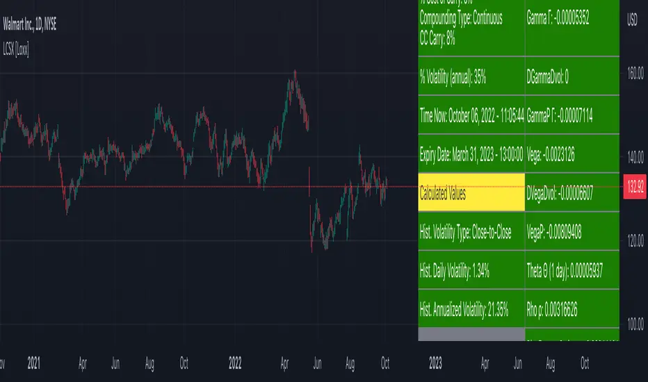
Reset Strike Options-Type 2 (Gray Whaley) [Loxx]For a reset option type 2, the strike is reset in a similar way as a reset option 1. That is, the strike is reset to the asset price at a predetermined future time, if the asset price is below (above) the initial strike price for a call (put). The payoff for such a reset call is max(S - X, 0), and max(X - S, 0) for a put, where X is equal to the original strike X if not reset, and equal to the reset strike if reset. Gray and Whaley (1999) have derived a closed-form solution for the price of European reset strike options. The price of the call option is then given by (via "The Complete Guide to Option Pricing Formulas")
c = Se^(b-r)T2 * M(a1, y1; p) - Xe^(-rT2) * M(a2, y2; p) - Se^(b-r)T1 * N(-a1) * N(z2) * e^-r(T2-T1) + Se^(b-r)T2 * N(-a1) * N(z1)
p = Se^(b-r)T1 * N(a1) * N(-z2) * e^-r(T2-T1) + Se^(b-r)T2 * N(a1) * N(-z1) + Xe^(-rT2) * M(-a2, -y2; p) - Se^(b-r)T2 * M(-a1, -y1; p)
where b is the cost-of-carry of the underlying asset, a is the volatility of the relative price changes in the asset, and r is the risk-free interest rate. K is the strike price of the option, T1 the time to reset (in years), and T2 is its time to expiration. N(x) and M(a,b; p) are, respectively, the univariate and bivariate cumulative normal distribution functions. Further
a1 = (log(S/X) + (b+v^2/2)T1) / v*T1^0.5 ... a2 = a1 - v*T1^0.5
z1 = ((b+v^2/2)(T2-T1)) / v*(T2-T1)^0.5 ... z2 = z1 - v*(T2-T1)^0.5
y1 = (log(S/X) + (b+v^2/2)T1) / v*T1^0.5 ... y2 = a1 - v*T1^0.5
and p = (T1/T2)^0.5. For reset options with multiple reset rights, see Dai, Kwok, and Wu (2003) and Liao and Wang (2003).
Inputs
Asset price ( S )
Strike price ( K )
Reset time ( T1 )
Time to maturity ( T2 )
Risk-free rate ( r )
Cost of carry ( b )
Volatility ( s )
Numerical Greeks or Greeks by Finite Difference
Analytical Greeks are the standard approach to estimating Delta, Gamma etc... That is what we typically use when we can derive from closed form solutions. Normally, these are well-defined and available in text books. Previously, we relied on closed form solutions for the call or put formulae differentiated with respect to the Black Scholes parameters. When Greeks formulae are difficult to develop or tease out, we can alternatively employ numerical Greeks - sometimes referred to finite difference approximations. A key advantage of numerical Greeks relates to their estimation independent of deriving mathematical Greeks. This could be important when we examine American options where there may not technically exist an exact closed form solution that is straightforward to work with. (via VinegarHill FinanceLabs)
Numerical Greeks Outputs
Delta D
Elasticity L
Gamma G
DGammaDvol
GammaP G
Vega
DvegaDvol
VegaP
Theta Q (1 day)
Rho r
Rho futures option r
Phi/Rho2
Carry
DDeltaDvol
Speed
Strike Delta
Strike gamma
Things to know
Only works on the daily timeframe and for the current source price.
You can adjust the text size to fit the screen

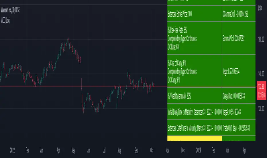
Writer Extendible Option [Loxx]These options can be exercised at their initial maturity date /I but are extended to T2 if the option is out-of-the-money at ti. The payoff from a writer-extendible call option at time T1 (T1 < T2) is (via "The Complete Guide to Option Pricing Formulas")
c(S, X1, X2, t1, T2) = (S - X1) if S>= X1 else cBSM(S, X2, T2-T1)
and for a writer-extendible put is
c(S, X1, X2, T1, T2) = (X1 - S) if S< X1 else pBSM(S, X2, T2-T1)
Writer-Extendible Call
c = cBSM(S, X1, T1) + Se^(b-r)T2 * M(Z1, -Z2; -p) - X2e^-rT2 * M(Z1 - vT^0.5, -Z2 + vT^0.5; -p)
Writer-Extendible Put
p = cBSM(S, X1, T1) + X2e^-rT2 * M(-Z1 + vT^0.5, Z2 - vT^0.5; -p) - Se^(b-r)T2 * M(-Z1, Z2; -p)
b=r options on non-dividend paying stock
b=r-q options on stock or index paying a dividend yield of q
b=0 options on futures
b=r-rf currency options (where rf is the rate in the second currency)
Inputs
Asset price ( S )
Initial strike price ( X1 )
Extended strike price ( X2 )
Initial time to maturity ( t1 )
Extended time to maturity ( T2 )
Risk-free rate ( r )
Cost of carry ( b )
Volatility ( s )
Numerical Greeks or Greeks by Finite Difference
Analytical Greeks are the standard approach to estimating Delta, Gamma etc... That is what we typically use when we can derive from closed form solutions. Normally, these are well-defined and available in text books. Previously, we relied on closed form solutions for the call or put formulae differentiated with respect to the Black Scholes parameters. When Greeks formulae are difficult to develop or tease out, we can alternatively employ numerical Greeks - sometimes referred to finite difference approximations. A key advantage of numerical Greeks relates to their estimation independent of deriving mathematical Greeks. This could be important when we examine American options where there may not technically exist an exact closed form solution that is straightforward to work with. (via VinegarHill FinanceLabs)
Numerical Greeks Output
Delta
Elasticity
Gamma
DGammaDvol
GammaP
Vega
DvegaDvol
VegaP
Theta (1 day)
Rho
Rho futures option
Phi/Rho2
Carry
DDeltaDvol
Speed
Things to know
Only works on the daily timeframe and for the current source price.
You can adjust the text size to fit the screen
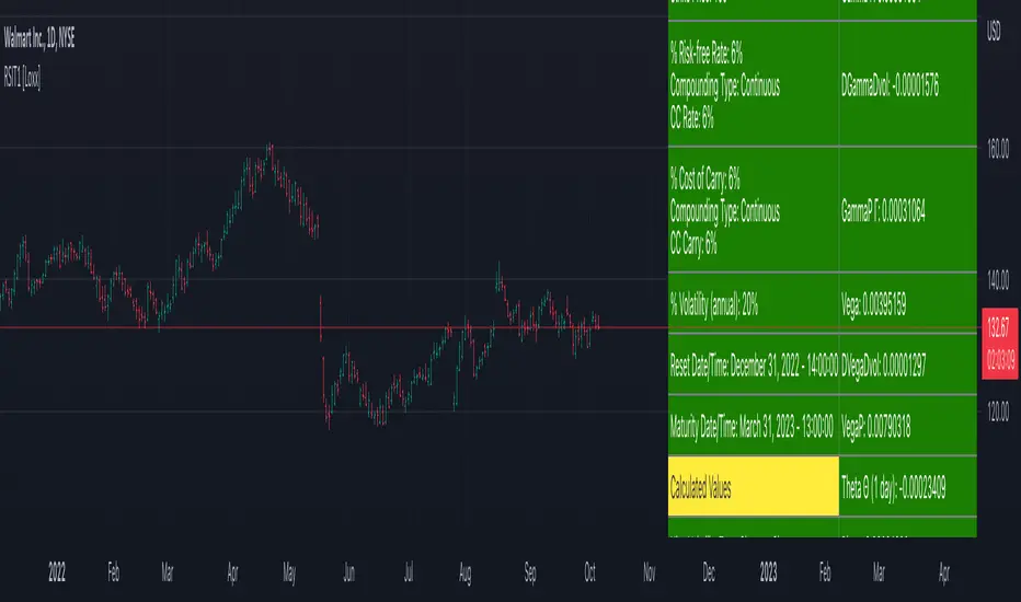
Reset Strike Options-Type 1 [Loxx]In a reset call (put) option, the strike is reset to the asset price at a predetermined future time, if the asset price is below (above) the initial strike price. This makes the strike path-dependent. The payoff for a call at maturity is equal to max((S-X)/X, 0) where is equal to the original strike X if not reset, and equal to the reset strike if reset. Similarly, for a put, the payoff is max((X-S)/X, 0) Gray and Whaley (1997) x have derived a closed-form solution for such an option. For a call, we have
c = e^(b-r)(T2-T1) * N(-a2) * N(z1) * e^(-rt1) - e^(-rT2) * N(-a2)*N(z2) - e^(-rT2) * M(a2, y2; p) + (S/X) * e^(b-r)T2 * M(a1, y1; p)
and for a put,
p = e^(-rT2) * N(a2) * N(-z2) - e^(b-r)(T2-T1) * N(a2) * N(-z1) * e^(-rT1) + e^(-rT2) * M(-a2, -y2; p) - (S/X) * e^(b-r)T2 * M(-a1, -y1; p)
where b is the cost-of-carry of the underlying asset, a is the volatil- ity of the relative price changes in the asset, and r is the risk-free interest rate. X is the strike price of the option, r the time to reset (in years), and T is its time to expiration. N(x) and M(a, b; p) are, respec- tively, the univariate and bivariate cumulative normal distribution functions. The remaining parameters are p = (T1/T2)^0.5 and
a1 = (log(S/X) + (b+v^2/2)T1) / vT1^0.5 ... a2 = a1 - vT1^0.5
z1 = (b+v^2/2)(T2-T1)/v(T2-T1)^0.5 ... z2 = z1 - v(T2-T1)^0.5
y1 = log(S/X) + (b+v^2)T2 / vT2^0.5 ... y2 = y1 - vT2^0.5
b=r options on non-dividend paying stock
b=r-q options on stock or index paying a dividend yield of q
b=0 options on futures
b=r-rf currency options (where rf is the rate in the second currency)
Inputs
Asset price ( S )
Initial strike price ( X1 )
Extended strike price ( X2 )
Initial time to maturity ( t1 )
Extended time to maturity ( T2 )
Risk-free rate ( r )
Cost of carry ( b )
Volatility ( s )
Numerical Greeks or Greeks by Finite Difference
Analytical Greeks are the standard approach to estimating Delta, Gamma etc... That is what we typically use when we can derive from closed form solutions. Normally, these are well-defined and available in text books. Previously, we relied on closed form solutions for the call or put formulae differentiated with respect to the Black Scholes parameters. When Greeks formulae are difficult to develop or tease out, we can alternatively employ numerical Greeks - sometimes referred to finite difference approximations. A key advantage of numerical Greeks relates to their estimation independent of deriving mathematical Greeks. This could be important when we examine American options where there may not technically exist an exact closed form solution that is straightforward to work with. (via VinegarHill FinanceLabs)
Numerical Greeks Ouput
Delta
Elasticity
Gamma
DGammaDvol
GammaP
Vega
DvegaDvol
VegaP
Theta (1 day)
Rho
Rho futures option
Phi/Rho2
Carry
DDeltaDvol
Speed
Things to know
Only works on the daily timeframe and for the current source price.
You can adjust the text size to fit the screen
Fade-in Options [Loxx]A fade-in call has the same payoff as a standard call except the size of the payoff is weighted by how many fixings the asset price were inside a predefined range (L, U). If the asset price is inside the range for every fixing, the payoff will be identical to a plain vanilla option. More precisely, for a call option, the payoff will be max(S(T) - X, 0) X 1/n Sum(n(i)), where n is the total number of fixings and n(i) = 1 if at fixing i the asset price is inside the range, and n(i) = 0 otherwise. Similarly, for a put, the payoff is max(X - S(T), 0) X 1/n Sum(n(i)).
Brockhaus, Ferraris, Gallus, Long, Martin, and Overhaus (1999) describe a closed-form formula for fade-in options. For a call the value is given by
max(X - S(T), 0) X 1/n Sum(n(i))
describe a closed-form formula for fade-in options. For a call the value is given by
c = 1/n * Sum(S^((b-r)*T) * (M(-d5, d1; -p) - M(-d3, d1; -p)) - Xe^(-rT) * (M(-d6, d2; -p) - M(-d4, d2; -p))
where n is the number of fixings, p = (t1^0.5/T^0.5), t1 = iT/n
d1 = (log(S/X) + (b + v^2/2)*T) / (v * T^0.5) ... d2 = d1 - v*T^0.5
d3 = (log(S/L) + (b + v^2/2)*t1) / (v * t1^0.5) ... d4 = d3 - v*t1^0.5
d5 = (log(S/U) + (b + v^2/2)*t1) / (v * t1^0.5) ... d6 = d5 - v*t1^0.5
The value of a put is similarly
p = 1/n * Sum(Xe^(-rT) * (M(-d6, -d2; -p) - M(-d4, -d2; -p))) - S^((b-r)*T) * (M(-d5, -d1; -p) - M(-d3, -d1; -p)
b=r options on non-dividend paying stock
b=r-q options on stock or index paying a dividend yield of q
b=0 options on futures
b=r-rf currency options (where rf is the rate in the second currency)
Inputs
Asset price ( S )
Strike price ( K )
Lower barrier ( L )
Upper barrier ( U )
Time to maturity ( T )
Risk-free rate ( r )
Cost of carry ( b )
Volatility ( s )
Fixings ( n )
cnd1(x) = Cumulative Normal Distribution
nd(x) = Standard Normal Density Function
cbnd3() = Cumulative Bivariate Distribution
convertingToCCRate(r, cmp ) = Rate compounder
Numerical Greeks or Greeks by Finite Difference
Analytical Greeks are the standard approach to estimating Delta, Gamma etc... That is what we typically use when we can derive from closed form solutions. Normally, these are well-defined and available in text books. Previously, we relied on closed form solutions for the call or put formulae differentiated with respect to the Black Scholes parameters. When Greeks formulae are difficult to develop or tease out, we can alternatively employ numerical Greeks - sometimes referred to finite difference approximations. A key advantage of numerical Greeks relates to their estimation independent of deriving mathematical Greeks. This could be important when we examine American options where there may not technically exist an exact closed form solution that is straightforward to work with. (via VinegarHill FinanceLabs)
Things to know
Only works on the daily timeframe and for the current source price.
You can adjust the text size to fit the screen

Log Contract Ln(S/X) [Loxx]A log contract, first introduced by Neuberger (1994) and Neuberger (1996), is not strictly an option. It is, however, an important building block in volatility derivatives (see Chapter 6 as well as Demeterfi, Derman, Kamal, and Zou, 1999). The payoff from a log contract at maturity T is simply the natural logarithm of the underlying asset divided by the strike price, ln(S/ X). The payoff is thus nonlinear and has many similarities with options. The value of this contract is (via "The Complete Guide to Option Pricing Formulas")
L = e^(-r * T) * (log(S/X) + (b-v^2/2)*T)
The delta of a log contract is
delta = (e^(-r*T) / S)
and the gamma is
gamma = (e^(-r*T) / S^2)
Inputs
S = Stock price.
K = Strike price of option.
T = Time to expiration in years.
r = Risk-free rate
c = Cost of Carry
V = Variance of the underlying asset price
cnd1(x) = Cumulative Normal Distribution
nd(x) = Standard Normal Density Function
convertingToCCRate(r, cmp ) = Rate compounder
Numerical Greeks or Greeks by Finite Difference
Analytical Greeks are the standard approach to estimating Delta, Gamma etc... That is what we typically use when we can derive from closed form solutions. Normally, these are well-defined and available in text books. Previously, we relied on closed form solutions for the call or put formulae differentiated with respect to the Black Scholes parameters. When Greeks formulae are difficult to develop or tease out, we can alternatively employ numerical Greeks - sometimes referred to finite difference approximations. A key advantage of numerical Greeks relates to their estimation independent of deriving mathematical Greeks. This could be important when we examine American options where there may not technically exist an exact closed form solution that is straightforward to work with. (via VinegarHill FinanceLabs)
Things to know
Only works on the daily timeframe and for the current source price.
You can adjust the text size to fit the screen
Log Option [Loxx]A log option introduced by Wilmott (2000) has a payoff at maturity equal to max(log(S/X), 0), which is basically an option on the rate of return on the underlying asset with strike log(X). The value of a log option is given by: (via "The Complete Guide to Option Pricing Formulas")
e^−rT * n(d2)σ√(T − t) + e^−rT*(log(S/K) + (b −σ^2/2)T) * N(d2)
where N(*) is the cumulative normal distribution function, n(*) is the normal density function, and
d = ((log(S/X) + (b - v^2/2)*T) / (v*T^0.5)
b=r options on non-dividend paying stock
b=r-q options on stock or index paying a dividend yield of q
b=0 options on futures
b=r-rf currency options (where rf is the rate in the second currency)
Inputs
S = Stock price.
K = Strike price of option.
T = Time to expiration in years.
r = Risk-free rate
c = Cost of Carry
V = Variance of the underlying asset price
cnd1(x) = Cumulative Normal Distribution
nd(x) = Standard Normal Density Function
convertingToCCRate(r, cmp ) = Rate compounder
Numerical Greeks or Greeks by Finite Difference
Analytical Greeks are the standard approach to estimating Delta, Gamma etc... That is what we typically use when we can derive from closed form solutions. Normally, these are well-defined and available in text books. Previously, we relied on closed form solutions for the call or put formulae differentiated with respect to the Black Scholes parameters. When Greeks formulae are difficult to develop or tease out, we can alternatively employ numerical Greeks - sometimes referred to finite difference approximations. A key advantage of numerical Greeks relates to their estimation independent of deriving mathematical Greeks. This could be important when we examine American options where there may not technically exist an exact closed form solution that is straightforward to work with. (via VinegarHill FinanceLabs)
Things to know
Only works on the daily timeframe and for the current source price.
You can adjust the text size to fit the screen