"williams"に関するスクリプトを検索

Williams Fractals by Sheridan Sadewa modif untuk menggunakan fractal yang ukurannya lebih kecil dan deket

Williams %R - Multi TimeframeThis indicator implements the William %R multi-timeframe. On the 1H chart, the curves for 1H (with signal), 4H, and 1D are displayed. On the 4H chart, the curves for 4H (with signal) and 1D are shown. On all other timeframes, only the %R and signal are displayed. The indicator is useful to use on 1H and 4H charts to find confluence among the different curves and identify better entries based on their alignment across all timeframes. Signals above 80 often indicate a potential bearish reversal in price, while signals below 20 often suggest a bullish price reversal.

Williams %R SKGThis is William% R indicator alongwith EMA and RSI overbought and oversold background


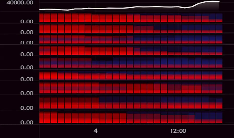
Williams Alligator Trend Filter HeatmapHello I've decided that the alligator lines can be used to find a trend. This script expands on that and checks 10 different multipliers to see trend over the long term and have 10 values. Those 10 values each give a color to one of the 10 lines in turn giving this Fire like plotting. I personaly use this to see if there is fear (red) in the markets or greed (blue), plotted 9 different crypto coins on the chart and have 4 columns in my setup to see the values on different timeframes. In the chart preview this is 1H,30M,10M,1M to see current environment. The colors use alot of data to generate especialy the bottom part, that colors based on a very long time zone.
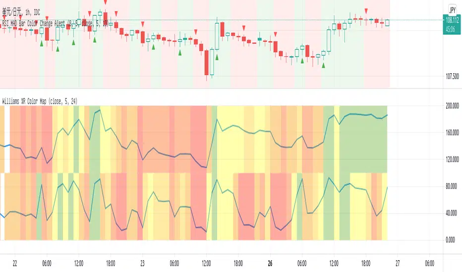
Williams %R Color MapThis script is used to have a quick view for my triple screen trading system.
I use it in 1 hour chart so that the higher timeframe is 5-hour and daily.
Visual for the current price on which fib area of 5-hour and daily chart.
Williams Gator Oscillator// The Gator Oscillator histogram above zero shows the absolute difference between blue and red lines of Alligator indicator,
// while histogram below zero shows the absolute difference between red and green lines.
//
// There are green and red bars on the Gator Oscillator histograms.
// A green bar appears when its value is higher than the value of the previous bar.
// A red bars appears when its value is lower than the value of the previous bar.
//
// Gator Oscillator helps to better visualize the upcoming changes in the trends: to know when Alligator sleeps, eats, fills //out and is about to go to sleep.

CCO_LibraryLibrary "CCO_Library"
Contrarian Crowd Oscillator (CCO) Library - Multi-oscillator consensus indicator for contrarian trading signals
@author B3AR_Trades
calculate_oscillators(rsi_length, stoch_length, cci_length, williams_length, roc_length, mfi_length, percentile_lookback, use_rsi, use_stochastic, use_williams, use_cci, use_roc, use_mfi)
Calculate normalized oscillator values
Parameters:
rsi_length (simple int) : (int) RSI calculation period
stoch_length (int) : (int) Stochastic calculation period
cci_length (int) : (int) CCI calculation period
williams_length (int) : (int) Williams %R calculation period
roc_length (int) : (int) ROC calculation period
mfi_length (int) : (int) MFI calculation period
percentile_lookback (int) : (int) Lookback period for CCI/ROC percentile ranking
use_rsi (bool) : (bool) Include RSI in calculations
use_stochastic (bool) : (bool) Include Stochastic in calculations
use_williams (bool) : (bool) Include Williams %R in calculations
use_cci (bool) : (bool) Include CCI in calculations
use_roc (bool) : (bool) Include ROC in calculations
use_mfi (bool) : (bool) Include MFI in calculations
Returns: (OscillatorValues) Normalized oscillator values
calculate_consensus_score(oscillators, use_rsi, use_stochastic, use_williams, use_cci, use_roc, use_mfi, weight_by_reliability, consensus_smoothing)
Calculate weighted consensus score
Parameters:
oscillators (OscillatorValues) : (OscillatorValues) Individual oscillator values
use_rsi (bool) : (bool) Include RSI in consensus
use_stochastic (bool) : (bool) Include Stochastic in consensus
use_williams (bool) : (bool) Include Williams %R in consensus
use_cci (bool) : (bool) Include CCI in consensus
use_roc (bool) : (bool) Include ROC in consensus
use_mfi (bool) : (bool) Include MFI in consensus
weight_by_reliability (bool) : (bool) Apply reliability-based weights
consensus_smoothing (int) : (int) Smoothing period for consensus
Returns: (float) Weighted consensus score (0-100)
calculate_consensus_strength(oscillators, consensus_score, use_rsi, use_stochastic, use_williams, use_cci, use_roc, use_mfi)
Calculate consensus strength (agreement between oscillators)
Parameters:
oscillators (OscillatorValues) : (OscillatorValues) Individual oscillator values
consensus_score (float) : (float) Current consensus score
use_rsi (bool) : (bool) Include RSI in strength calculation
use_stochastic (bool) : (bool) Include Stochastic in strength calculation
use_williams (bool) : (bool) Include Williams %R in strength calculation
use_cci (bool) : (bool) Include CCI in strength calculation
use_roc (bool) : (bool) Include ROC in strength calculation
use_mfi (bool) : (bool) Include MFI in strength calculation
Returns: (float) Consensus strength (0-100)
classify_regime(consensus_score)
Classify consensus regime
Parameters:
consensus_score (float) : (float) Current consensus score
Returns: (ConsensusRegime) Regime classification
detect_signals(consensus_score, consensus_strength, consensus_momentum, regime)
Detect trading signals
Parameters:
consensus_score (float) : (float) Current consensus score
consensus_strength (float) : (float) Current consensus strength
consensus_momentum (float) : (float) Consensus momentum
regime (ConsensusRegime) : (ConsensusRegime) Current regime classification
Returns: (TradingSignals) Trading signal conditions
calculate_cco(rsi_length, stoch_length, cci_length, williams_length, roc_length, mfi_length, consensus_smoothing, percentile_lookback, use_rsi, use_stochastic, use_williams, use_cci, use_roc, use_mfi, weight_by_reliability, detect_momentum)
Calculate complete CCO analysis
Parameters:
rsi_length (simple int) : (int) RSI calculation period
stoch_length (int) : (int) Stochastic calculation period
cci_length (int) : (int) CCI calculation period
williams_length (int) : (int) Williams %R calculation period
roc_length (int) : (int) ROC calculation period
mfi_length (int) : (int) MFI calculation period
consensus_smoothing (int) : (int) Consensus smoothing period
percentile_lookback (int) : (int) Percentile ranking lookback
use_rsi (bool) : (bool) Include RSI
use_stochastic (bool) : (bool) Include Stochastic
use_williams (bool) : (bool) Include Williams %R
use_cci (bool) : (bool) Include CCI
use_roc (bool) : (bool) Include ROC
use_mfi (bool) : (bool) Include MFI
weight_by_reliability (bool) : (bool) Apply reliability weights
detect_momentum (bool) : (bool) Calculate momentum and acceleration
Returns: (CCOResult) Complete CCO analysis results
calculate_cco_default()
Calculate CCO with default parameters
Returns: (CCOResult) CCO result with standard settings
cco_consensus_score()
Get just the consensus score with default parameters
Returns: (float) Consensus score (0-100)
cco_consensus_strength()
Get just the consensus strength with default parameters
Returns: (float) Consensus strength (0-100)
is_panic_bottom()
Check if in panic bottom condition
Returns: (bool) True if panic bottom signal active
is_euphoric_top()
Check if in euphoric top condition
Returns: (bool) True if euphoric top signal active
bullish_consensus_reversal()
Check for bullish consensus reversal
Returns: (bool) True if bullish reversal detected
bearish_consensus_reversal()
Check for bearish consensus reversal
Returns: (bool) True if bearish reversal detected
bearish_divergence()
Check for bearish divergence
Returns: (bool) True if bearish divergence detected
bullish_divergence()
Check for bullish divergence
Returns: (bool) True if bullish divergence detected
get_regime_name()
Get current regime name
Returns: (string) Current consensus regime name
get_contrarian_signal()
Get contrarian signal
Returns: (string) Current contrarian trading signal
get_position_multiplier()
Get position size multiplier
Returns: (float) Recommended position sizing multiplier
OscillatorValues
Individual oscillator values
Fields:
rsi (series float) : RSI value (0-100)
stochastic (series float) : Stochastic value (0-100)
williams (series float) : Williams %R value (0-100, normalized)
cci (series float) : CCI percentile value (0-100)
roc (series float) : ROC percentile value (0-100)
mfi (series float) : Money Flow Index value (0-100)
ConsensusRegime
Consensus regime classification
Fields:
extreme_bearish (series bool) : Extreme bearish consensus (<= 20)
moderate_bearish (series bool) : Moderate bearish consensus (20-40)
mixed (series bool) : Mixed consensus (40-60)
moderate_bullish (series bool) : Moderate bullish consensus (60-80)
extreme_bullish (series bool) : Extreme bullish consensus (>= 80)
regime_name (series string) : Text description of current regime
contrarian_signal (series string) : Contrarian trading signal
TradingSignals
Trading signals
Fields:
panic_bottom_signal (series bool) : Extreme bearish consensus with high strength
euphoric_top_signal (series bool) : Extreme bullish consensus with high strength
consensus_reversal_bullish (series bool) : Bullish consensus reversal
consensus_reversal_bearish (series bool) : Bearish consensus reversal
bearish_divergence (series bool) : Bearish price-consensus divergence
bullish_divergence (series bool) : Bullish price-consensus divergence
strong_consensus (series bool) : High consensus strength signal
CCOResult
Complete CCO calculation results
Fields:
consensus_score (series float) : Main consensus score (0-100)
consensus_strength (series float) : Consensus strength (0-100)
consensus_momentum (series float) : Rate of consensus change
consensus_acceleration (series float) : Rate of momentum change
oscillators (OscillatorValues) : Individual oscillator values
regime (ConsensusRegime) : Regime classification
signals (TradingSignals) : Trading signals
position_multiplier (series float) : Recommended position sizing multiplier

Markov Chain [3D] | FractalystWhat exactly is a Markov Chain?
This indicator uses a Markov Chain model to analyze, quantify, and visualize the transitions between market regimes (Bull, Bear, Neutral) on your chart. It dynamically detects these regimes in real-time, calculates transition probabilities, and displays them as animated 3D spheres and arrows, giving traders intuitive insight into current and future market conditions.
How does a Markov Chain work, and how should I read this spheres-and-arrows diagram?
Think of three weather modes: Sunny, Rainy, Cloudy.
Each sphere is one mode. The loop on a sphere means “stay the same next step” (e.g., Sunny again tomorrow).
The arrows leaving a sphere show where things usually go next if they change (e.g., Sunny moving to Cloudy).
Some paths matter more than others. A more prominent loop means the current mode tends to persist. A more prominent outgoing arrow means a change to that destination is the usual next step.
Direction isn’t symmetric: moving Sunny→Cloudy can behave differently than Cloudy→Sunny.
Now relabel the spheres to markets: Bull, Bear, Neutral.
Spheres: market regimes (uptrend, downtrend, range).
Self‑loop: tendency for the current regime to continue on the next bar.
Arrows: the most common next regime if a switch happens.
How to read: Start at the sphere that matches current bar state. If the loop stands out, expect continuation. If one outgoing path stands out, that switch is the typical next step. Opposite directions can differ (Bear→Neutral doesn’t have to match Neutral→Bear).
What states and transitions are shown?
The three market states visualized are:
Bullish (Bull): Upward or strong-market regime.
Bearish (Bear): Downward or weak-market regime.
Neutral: Sideways or range-bound regime.
Bidirectional animated arrows and probability labels show how likely the market is to move from one regime to another (e.g., Bull → Bear or Neutral → Bull).
How does the regime detection system work?
You can use either built-in price returns (based on adaptive Z-score normalization) or supply three custom indicators (such as volume, oscillators, etc.).
Values are statistically normalized (Z-scored) over a configurable lookback period.
The normalized outputs are classified into Bull, Bear, or Neutral zones.
If using three indicators, their regime signals are averaged and smoothed for robustness.
How are transition probabilities calculated?
On every confirmed bar, the algorithm tracks the sequence of detected market states, then builds a rolling window of transitions.
The code maintains a transition count matrix for all regime pairs (e.g., Bull → Bear).
Transition probabilities are extracted for each possible state change using Laplace smoothing for numerical stability, and frequently updated in real-time.
What is unique about the visualization?
3D animated spheres represent each regime and change visually when active.
Animated, bidirectional arrows reveal transition probabilities and allow you to see both dominant and less likely regime flows.
Particles (moving dots) animate along the arrows, enhancing the perception of regime flow direction and speed.
All elements dynamically update with each new price bar, providing a live market map in an intuitive, engaging format.
Can I use custom indicators for regime classification?
Yes! Enable the "Custom Indicators" switch and select any three chart series as inputs. These will be normalized and combined (each with equal weight), broadening the regime classification beyond just price-based movement.
What does the “Lookback Period” control?
Lookback Period (default: 100) sets how much historical data builds the probability matrix. Shorter periods adapt faster to regime changes but may be noisier. Longer periods are more stable but slower to adapt.
How is this different from a Hidden Markov Model (HMM)?
It sets the window for both regime detection and probability calculations. Lower values make the system more reactive, but potentially noisier. Higher values smooth estimates and make the system more robust.
How is this Markov Chain different from a Hidden Markov Model (HMM)?
Markov Chain (as here): All market regimes (Bull, Bear, Neutral) are directly observable on the chart. The transition matrix is built from actual detected regimes, keeping the model simple and interpretable.
Hidden Markov Model: The actual regimes are unobservable ("hidden") and must be inferred from market output or indicator "emissions" using statistical learning algorithms. HMMs are more complex, can capture more subtle structure, but are harder to visualize and require additional machine learning steps for training.
A standard Markov Chain models transitions between observable states using a simple transition matrix, while a Hidden Markov Model assumes the true states are hidden (latent) and must be inferred from observable “emissions” like price or volume data. In practical terms, a Markov Chain is transparent and easier to implement and interpret; an HMM is more expressive but requires statistical inference to estimate hidden states from data.
Markov Chain: states are observable; you directly count or estimate transition probabilities between visible states. This makes it simpler, faster, and easier to validate and tune.
HMM: states are hidden; you only observe emissions generated by those latent states. Learning involves machine learning/statistical algorithms (commonly Baum–Welch/EM for training and Viterbi for decoding) to infer both the transition dynamics and the most likely hidden state sequence from data.
How does the indicator avoid “repainting” or look-ahead bias?
All regime changes and matrix updates happen only on confirmed (closed) bars, so no future data is leaked, ensuring reliable real-time operation.
Are there practical tuning tips?
Tune the Lookback Period for your asset/timeframe: shorter for fast markets, longer for stability.
Use custom indicators if your asset has unique regime drivers.
Watch for rapid changes in transition probabilities as early warning of a possible regime shift.
Who is this indicator for?
Quants and quantitative researchers exploring probabilistic market modeling, especially those interested in regime-switching dynamics and Markov models.
Programmers and system developers who need a probabilistic regime filter for systematic and algorithmic backtesting:
The Markov Chain indicator is ideally suited for programmatic integration via its bias output (1 = Bull, 0 = Neutral, -1 = Bear).
Although the visualization is engaging, the core output is designed for automated, rules-based workflows—not for discretionary/manual trading decisions.
Developers can connect the indicator’s output directly to their Pine Script logic (using input.source()), allowing rapid and robust backtesting of regime-based strategies.
It acts as a plug-and-play regime filter: simply plug the bias output into your entry/exit logic, and you have a scientifically robust, probabilistically-derived signal for filtering, timing, position sizing, or risk regimes.
The MC's output is intentionally "trinary" (1/0/-1), focusing on clear regime states for unambiguous decision-making in code. If you require nuanced, multi-probability or soft-label state vectors, consider expanding the indicator or stacking it with a probability-weighted logic layer in your scripting.
Because it avoids subjectivity, this approach is optimal for systematic quants, algo developers building backtested, repeatable strategies based on probabilistic regime analysis.
What's the mathematical foundation behind this?
The mathematical foundation behind this Markov Chain indicator—and probabilistic regime detection in finance—draws from two principal models: the (standard) Markov Chain and the Hidden Markov Model (HMM).
How to use this indicator programmatically?
The Markov Chain indicator automatically exports a bias value (+1 for Bullish, -1 for Bearish, 0 for Neutral) as a plot visible in the Data Window. This allows you to integrate its regime signal into your own scripts and strategies for backtesting, automation, or live trading.
Step-by-Step Integration with Pine Script (input.source)
Add the Markov Chain indicator to your chart.
This must be done first, since your custom script will "pull" the bias signal from the indicator's plot.
In your strategy, create an input using input.source()
Example:
//@version=5
strategy("MC Bias Strategy Example")
mcBias = input.source(close, "MC Bias Source")
After saving, go to your script’s settings. For the “MC Bias Source” input, select the plot/output of the Markov Chain indicator (typically its bias plot).
Use the bias in your trading logic
Example (long only on Bull, flat otherwise):
if mcBias == 1
strategy.entry("Long", strategy.long)
else
strategy.close("Long")
For more advanced workflows, combine mcBias with additional filters or trailing stops.
How does this work behind-the-scenes?
TradingView’s input.source() lets you use any plot from another indicator as a real-time, “live” data feed in your own script (source).
The selected bias signal is available to your Pine code as a variable, enabling logical decisions based on regime (trend-following, mean-reversion, etc.).
This enables powerful strategy modularity : decouple regime detection from entry/exit logic, allowing fast experimentation without rewriting core signal code.
Integrating 45+ Indicators with Your Markov Chain — How & Why
The Enhanced Custom Indicators Export script exports a massive suite of over 45 technical indicators—ranging from classic momentum (RSI, MACD, Stochastic, etc.) to trend, volume, volatility, and oscillator tools—all pre-calculated, centered/scaled, and available as plots.
// Enhanced Custom Indicators Export - 45 Technical Indicators
// Comprehensive technical analysis suite for advanced market regime detection
//@version=6
indicator('Enhanced Custom Indicators Export | Fractalyst', shorttitle='Enhanced CI Export', overlay=false, scale=scale.right, max_labels_count=500, max_lines_count=500)
// |----- Input Parameters -----| //
momentum_group = "Momentum Indicators"
trend_group = "Trend Indicators"
volume_group = "Volume Indicators"
volatility_group = "Volatility Indicators"
oscillator_group = "Oscillator Indicators"
display_group = "Display Settings"
// Common lengths
length_14 = input.int(14, "Standard Length (14)", minval=1, maxval=100, group=momentum_group)
length_20 = input.int(20, "Medium Length (20)", minval=1, maxval=200, group=trend_group)
length_50 = input.int(50, "Long Length (50)", minval=1, maxval=200, group=trend_group)
// Display options
show_table = input.bool(true, "Show Values Table", group=display_group)
table_size = input.string("Small", "Table Size", options= , group=display_group)
// |----- MOMENTUM INDICATORS (15 indicators) -----| //
// 1. RSI (Relative Strength Index)
rsi_14 = ta.rsi(close, length_14)
rsi_centered = rsi_14 - 50
// 2. Stochastic Oscillator
stoch_k = ta.stoch(close, high, low, length_14)
stoch_d = ta.sma(stoch_k, 3)
stoch_centered = stoch_k - 50
// 3. Williams %R
williams_r = ta.stoch(close, high, low, length_14) - 100
// 4. MACD (Moving Average Convergence Divergence)
= ta.macd(close, 12, 26, 9)
// 5. Momentum (Rate of Change)
momentum = ta.mom(close, length_14)
momentum_pct = (momentum / close ) * 100
// 6. Rate of Change (ROC)
roc = ta.roc(close, length_14)
// 7. Commodity Channel Index (CCI)
cci = ta.cci(close, length_20)
// 8. Money Flow Index (MFI)
mfi = ta.mfi(close, length_14)
mfi_centered = mfi - 50
// 9. Awesome Oscillator (AO)
ao = ta.sma(hl2, 5) - ta.sma(hl2, 34)
// 10. Accelerator Oscillator (AC)
ac = ao - ta.sma(ao, 5)
// 11. Chande Momentum Oscillator (CMO)
cmo = ta.cmo(close, length_14)
// 12. Detrended Price Oscillator (DPO)
dpo = close - ta.sma(close, length_20)
// 13. Price Oscillator (PPO)
ppo = ta.sma(close, 12) - ta.sma(close, 26)
ppo_pct = (ppo / ta.sma(close, 26)) * 100
// 14. TRIX
trix_ema1 = ta.ema(close, length_14)
trix_ema2 = ta.ema(trix_ema1, length_14)
trix_ema3 = ta.ema(trix_ema2, length_14)
trix = ta.roc(trix_ema3, 1) * 10000
// 15. Klinger Oscillator
klinger = ta.ema(volume * (high + low + close) / 3, 34) - ta.ema(volume * (high + low + close) / 3, 55)
// 16. Fisher Transform
fisher_hl2 = 0.5 * (hl2 - ta.lowest(hl2, 10)) / (ta.highest(hl2, 10) - ta.lowest(hl2, 10)) - 0.25
fisher = 0.5 * math.log((1 + fisher_hl2) / (1 - fisher_hl2))
// 17. Stochastic RSI
stoch_rsi = ta.stoch(rsi_14, rsi_14, rsi_14, length_14)
stoch_rsi_centered = stoch_rsi - 50
// 18. Relative Vigor Index (RVI)
rvi_num = ta.swma(close - open)
rvi_den = ta.swma(high - low)
rvi = rvi_den != 0 ? rvi_num / rvi_den : 0
// 19. Balance of Power (BOP)
bop = (close - open) / (high - low)
// |----- TREND INDICATORS (10 indicators) -----| //
// 20. Simple Moving Average Momentum
sma_20 = ta.sma(close, length_20)
sma_momentum = ((close - sma_20) / sma_20) * 100
// 21. Exponential Moving Average Momentum
ema_20 = ta.ema(close, length_20)
ema_momentum = ((close - ema_20) / ema_20) * 100
// 22. Parabolic SAR
sar = ta.sar(0.02, 0.02, 0.2)
sar_trend = close > sar ? 1 : -1
// 23. Linear Regression Slope
lr_slope = ta.linreg(close, length_20, 0) - ta.linreg(close, length_20, 1)
// 24. Moving Average Convergence (MAC)
mac = ta.sma(close, 10) - ta.sma(close, 30)
// 25. Trend Intensity Index (TII)
tii_sum = 0.0
for i = 1 to length_20
tii_sum += close > close ? 1 : 0
tii = (tii_sum / length_20) * 100
// 26. Ichimoku Cloud Components
ichimoku_tenkan = (ta.highest(high, 9) + ta.lowest(low, 9)) / 2
ichimoku_kijun = (ta.highest(high, 26) + ta.lowest(low, 26)) / 2
ichimoku_signal = ichimoku_tenkan > ichimoku_kijun ? 1 : -1
// 27. MESA Adaptive Moving Average (MAMA)
mama_alpha = 2.0 / (length_20 + 1)
mama = ta.ema(close, length_20)
mama_momentum = ((close - mama) / mama) * 100
// 28. Zero Lag Exponential Moving Average (ZLEMA)
zlema_lag = math.round((length_20 - 1) / 2)
zlema_data = close + (close - close )
zlema = ta.ema(zlema_data, length_20)
zlema_momentum = ((close - zlema) / zlema) * 100
// |----- VOLUME INDICATORS (6 indicators) -----| //
// 29. On-Balance Volume (OBV)
obv = ta.obv
// 30. Volume Rate of Change (VROC)
vroc = ta.roc(volume, length_14)
// 31. Price Volume Trend (PVT)
pvt = ta.pvt
// 32. Negative Volume Index (NVI)
nvi = 0.0
nvi := volume < volume ? nvi + ((close - close ) / close ) * nvi : nvi
// 33. Positive Volume Index (PVI)
pvi = 0.0
pvi := volume > volume ? pvi + ((close - close ) / close ) * pvi : pvi
// 34. Volume Oscillator
vol_osc = ta.sma(volume, 5) - ta.sma(volume, 10)
// 35. Ease of Movement (EOM)
eom_distance = high - low
eom_box_height = volume / 1000000
eom = eom_box_height != 0 ? eom_distance / eom_box_height : 0
eom_sma = ta.sma(eom, length_14)
// 36. Force Index
force_index = volume * (close - close )
force_index_sma = ta.sma(force_index, length_14)
// |----- VOLATILITY INDICATORS (10 indicators) -----| //
// 37. Average True Range (ATR)
atr = ta.atr(length_14)
atr_pct = (atr / close) * 100
// 38. Bollinger Bands Position
bb_basis = ta.sma(close, length_20)
bb_dev = 2.0 * ta.stdev(close, length_20)
bb_upper = bb_basis + bb_dev
bb_lower = bb_basis - bb_dev
bb_position = bb_dev != 0 ? (close - bb_basis) / bb_dev : 0
bb_width = bb_dev != 0 ? (bb_upper - bb_lower) / bb_basis * 100 : 0
// 39. Keltner Channels Position
kc_basis = ta.ema(close, length_20)
kc_range = ta.ema(ta.tr, length_20)
kc_upper = kc_basis + (2.0 * kc_range)
kc_lower = kc_basis - (2.0 * kc_range)
kc_position = kc_range != 0 ? (close - kc_basis) / kc_range : 0
// 40. Donchian Channels Position
dc_upper = ta.highest(high, length_20)
dc_lower = ta.lowest(low, length_20)
dc_basis = (dc_upper + dc_lower) / 2
dc_position = (dc_upper - dc_lower) != 0 ? (close - dc_basis) / (dc_upper - dc_lower) : 0
// 41. Standard Deviation
std_dev = ta.stdev(close, length_20)
std_dev_pct = (std_dev / close) * 100
// 42. Relative Volatility Index (RVI)
rvi_up = ta.stdev(close > close ? close : 0, length_14)
rvi_down = ta.stdev(close < close ? close : 0, length_14)
rvi_total = rvi_up + rvi_down
rvi_volatility = rvi_total != 0 ? (rvi_up / rvi_total) * 100 : 50
// 43. Historical Volatility
hv_returns = math.log(close / close )
hv = ta.stdev(hv_returns, length_20) * math.sqrt(252) * 100
// 44. Garman-Klass Volatility
gk_vol = math.log(high/low) * math.log(high/low) - (2*math.log(2)-1) * math.log(close/open) * math.log(close/open)
gk_volatility = math.sqrt(ta.sma(gk_vol, length_20)) * 100
// 45. Parkinson Volatility
park_vol = math.log(high/low) * math.log(high/low)
parkinson = math.sqrt(ta.sma(park_vol, length_20) / (4 * math.log(2))) * 100
// 46. Rogers-Satchell Volatility
rs_vol = math.log(high/close) * math.log(high/open) + math.log(low/close) * math.log(low/open)
rogers_satchell = math.sqrt(ta.sma(rs_vol, length_20)) * 100
// |----- OSCILLATOR INDICATORS (5 indicators) -----| //
// 47. Elder Ray Index
elder_bull = high - ta.ema(close, 13)
elder_bear = low - ta.ema(close, 13)
elder_power = elder_bull + elder_bear
// 48. Schaff Trend Cycle (STC)
stc_macd = ta.ema(close, 23) - ta.ema(close, 50)
stc_k = ta.stoch(stc_macd, stc_macd, stc_macd, 10)
stc_d = ta.ema(stc_k, 3)
stc = ta.stoch(stc_d, stc_d, stc_d, 10)
// 49. Coppock Curve
coppock_roc1 = ta.roc(close, 14)
coppock_roc2 = ta.roc(close, 11)
coppock = ta.wma(coppock_roc1 + coppock_roc2, 10)
// 50. Know Sure Thing (KST)
kst_roc1 = ta.roc(close, 10)
kst_roc2 = ta.roc(close, 15)
kst_roc3 = ta.roc(close, 20)
kst_roc4 = ta.roc(close, 30)
kst = ta.sma(kst_roc1, 10) + 2*ta.sma(kst_roc2, 10) + 3*ta.sma(kst_roc3, 10) + 4*ta.sma(kst_roc4, 15)
// 51. Percentage Price Oscillator (PPO)
ppo_line = ((ta.ema(close, 12) - ta.ema(close, 26)) / ta.ema(close, 26)) * 100
ppo_signal = ta.ema(ppo_line, 9)
ppo_histogram = ppo_line - ppo_signal
// |----- PLOT MAIN INDICATORS -----| //
// Plot key momentum indicators
plot(rsi_centered, title="01_RSI_Centered", color=color.purple, linewidth=1)
plot(stoch_centered, title="02_Stoch_Centered", color=color.blue, linewidth=1)
plot(williams_r, title="03_Williams_R", color=color.red, linewidth=1)
plot(macd_histogram, title="04_MACD_Histogram", color=color.orange, linewidth=1)
plot(cci, title="05_CCI", color=color.green, linewidth=1)
// Plot trend indicators
plot(sma_momentum, title="06_SMA_Momentum", color=color.navy, linewidth=1)
plot(ema_momentum, title="07_EMA_Momentum", color=color.maroon, linewidth=1)
plot(sar_trend, title="08_SAR_Trend", color=color.teal, linewidth=1)
plot(lr_slope, title="09_LR_Slope", color=color.lime, linewidth=1)
plot(mac, title="10_MAC", color=color.fuchsia, linewidth=1)
// Plot volatility indicators
plot(atr_pct, title="11_ATR_Pct", color=color.yellow, linewidth=1)
plot(bb_position, title="12_BB_Position", color=color.aqua, linewidth=1)
plot(kc_position, title="13_KC_Position", color=color.olive, linewidth=1)
plot(std_dev_pct, title="14_StdDev_Pct", color=color.silver, linewidth=1)
plot(bb_width, title="15_BB_Width", color=color.gray, linewidth=1)
// Plot volume indicators
plot(vroc, title="16_VROC", color=color.blue, linewidth=1)
plot(eom_sma, title="17_EOM", color=color.red, linewidth=1)
plot(vol_osc, title="18_Vol_Osc", color=color.green, linewidth=1)
plot(force_index_sma, title="19_Force_Index", color=color.orange, linewidth=1)
plot(obv, title="20_OBV", color=color.purple, linewidth=1)
// Plot additional oscillators
plot(ao, title="21_Awesome_Osc", color=color.navy, linewidth=1)
plot(cmo, title="22_CMO", color=color.maroon, linewidth=1)
plot(dpo, title="23_DPO", color=color.teal, linewidth=1)
plot(trix, title="24_TRIX", color=color.lime, linewidth=1)
plot(fisher, title="25_Fisher", color=color.fuchsia, linewidth=1)
// Plot more momentum indicators
plot(mfi_centered, title="26_MFI_Centered", color=color.yellow, linewidth=1)
plot(ac, title="27_AC", color=color.aqua, linewidth=1)
plot(ppo_pct, title="28_PPO_Pct", color=color.olive, linewidth=1)
plot(stoch_rsi_centered, title="29_StochRSI_Centered", color=color.silver, linewidth=1)
plot(klinger, title="30_Klinger", color=color.gray, linewidth=1)
// Plot trend continuation
plot(tii, title="31_TII", color=color.blue, linewidth=1)
plot(ichimoku_signal, title="32_Ichimoku_Signal", color=color.red, linewidth=1)
plot(mama_momentum, title="33_MAMA_Momentum", color=color.green, linewidth=1)
plot(zlema_momentum, title="34_ZLEMA_Momentum", color=color.orange, linewidth=1)
plot(bop, title="35_BOP", color=color.purple, linewidth=1)
// Plot volume continuation
plot(nvi, title="36_NVI", color=color.navy, linewidth=1)
plot(pvi, title="37_PVI", color=color.maroon, linewidth=1)
plot(momentum_pct, title="38_Momentum_Pct", color=color.teal, linewidth=1)
plot(roc, title="39_ROC", color=color.lime, linewidth=1)
plot(rvi, title="40_RVI", color=color.fuchsia, linewidth=1)
// Plot volatility continuation
plot(dc_position, title="41_DC_Position", color=color.yellow, linewidth=1)
plot(rvi_volatility, title="42_RVI_Volatility", color=color.aqua, linewidth=1)
plot(hv, title="43_Historical_Vol", color=color.olive, linewidth=1)
plot(gk_volatility, title="44_GK_Volatility", color=color.silver, linewidth=1)
plot(parkinson, title="45_Parkinson_Vol", color=color.gray, linewidth=1)
// Plot final oscillators
plot(rogers_satchell, title="46_RS_Volatility", color=color.blue, linewidth=1)
plot(elder_power, title="47_Elder_Power", color=color.red, linewidth=1)
plot(stc, title="48_STC", color=color.green, linewidth=1)
plot(coppock, title="49_Coppock", color=color.orange, linewidth=1)
plot(kst, title="50_KST", color=color.purple, linewidth=1)
// Plot final indicators
plot(ppo_histogram, title="51_PPO_Histogram", color=color.navy, linewidth=1)
plot(pvt, title="52_PVT", color=color.maroon, linewidth=1)
// |----- Reference Lines -----| //
hline(0, "Zero Line", color=color.gray, linestyle=hline.style_dashed, linewidth=1)
hline(50, "Midline", color=color.gray, linestyle=hline.style_dotted, linewidth=1)
hline(-50, "Lower Midline", color=color.gray, linestyle=hline.style_dotted, linewidth=1)
hline(25, "Upper Threshold", color=color.gray, linestyle=hline.style_dotted, linewidth=1)
hline(-25, "Lower Threshold", color=color.gray, linestyle=hline.style_dotted, linewidth=1)
// |----- Enhanced Information Table -----| //
if show_table and barstate.islast
table_position = position.top_right
table_text_size = table_size == "Tiny" ? size.tiny : table_size == "Small" ? size.small : size.normal
var table info_table = table.new(table_position, 3, 18, bgcolor=color.new(color.white, 85), border_width=1, border_color=color.gray)
// Headers
table.cell(info_table, 0, 0, 'Category', text_color=color.black, text_size=table_text_size, bgcolor=color.new(color.blue, 70))
table.cell(info_table, 1, 0, 'Indicator', text_color=color.black, text_size=table_text_size, bgcolor=color.new(color.blue, 70))
table.cell(info_table, 2, 0, 'Value', text_color=color.black, text_size=table_text_size, bgcolor=color.new(color.blue, 70))
// Key Momentum Indicators
table.cell(info_table, 0, 1, 'MOMENTUM', text_color=color.purple, text_size=table_text_size, bgcolor=color.new(color.purple, 90))
table.cell(info_table, 1, 1, 'RSI Centered', text_color=color.purple, text_size=table_text_size)
table.cell(info_table, 2, 1, str.tostring(rsi_centered, '0.00'), text_color=color.purple, text_size=table_text_size)
table.cell(info_table, 0, 2, '', text_color=color.blue, text_size=table_text_size)
table.cell(info_table, 1, 2, 'Stoch Centered', text_color=color.blue, text_size=table_text_size)
table.cell(info_table, 2, 2, str.tostring(stoch_centered, '0.00'), text_color=color.blue, text_size=table_text_size)
table.cell(info_table, 0, 3, '', text_color=color.red, text_size=table_text_size)
table.cell(info_table, 1, 3, 'Williams %R', text_color=color.red, text_size=table_text_size)
table.cell(info_table, 2, 3, str.tostring(williams_r, '0.00'), text_color=color.red, text_size=table_text_size)
table.cell(info_table, 0, 4, '', text_color=color.orange, text_size=table_text_size)
table.cell(info_table, 1, 4, 'MACD Histogram', text_color=color.orange, text_size=table_text_size)
table.cell(info_table, 2, 4, str.tostring(macd_histogram, '0.000'), text_color=color.orange, text_size=table_text_size)
table.cell(info_table, 0, 5, '', text_color=color.green, text_size=table_text_size)
table.cell(info_table, 1, 5, 'CCI', text_color=color.green, text_size=table_text_size)
table.cell(info_table, 2, 5, str.tostring(cci, '0.00'), text_color=color.green, text_size=table_text_size)
// Key Trend Indicators
table.cell(info_table, 0, 6, 'TREND', text_color=color.navy, text_size=table_text_size, bgcolor=color.new(color.navy, 90))
table.cell(info_table, 1, 6, 'SMA Momentum %', text_color=color.navy, text_size=table_text_size)
table.cell(info_table, 2, 6, str.tostring(sma_momentum, '0.00'), text_color=color.navy, text_size=table_text_size)
table.cell(info_table, 0, 7, '', text_color=color.maroon, text_size=table_text_size)
table.cell(info_table, 1, 7, 'EMA Momentum %', text_color=color.maroon, text_size=table_text_size)
table.cell(info_table, 2, 7, str.tostring(ema_momentum, '0.00'), text_color=color.maroon, text_size=table_text_size)
table.cell(info_table, 0, 8, '', text_color=color.teal, text_size=table_text_size)
table.cell(info_table, 1, 8, 'SAR Trend', text_color=color.teal, text_size=table_text_size)
table.cell(info_table, 2, 8, str.tostring(sar_trend, '0'), text_color=color.teal, text_size=table_text_size)
table.cell(info_table, 0, 9, '', text_color=color.lime, text_size=table_text_size)
table.cell(info_table, 1, 9, 'Linear Regression', text_color=color.lime, text_size=table_text_size)
table.cell(info_table, 2, 9, str.tostring(lr_slope, '0.000'), text_color=color.lime, text_size=table_text_size)
// Key Volatility Indicators
table.cell(info_table, 0, 10, 'VOLATILITY', text_color=color.yellow, text_size=table_text_size, bgcolor=color.new(color.yellow, 90))
table.cell(info_table, 1, 10, 'ATR %', text_color=color.yellow, text_size=table_text_size)
table.cell(info_table, 2, 10, str.tostring(atr_pct, '0.00'), text_color=color.yellow, text_size=table_text_size)
table.cell(info_table, 0, 11, '', text_color=color.aqua, text_size=table_text_size)
table.cell(info_table, 1, 11, 'BB Position', text_color=color.aqua, text_size=table_text_size)
table.cell(info_table, 2, 11, str.tostring(bb_position, '0.00'), text_color=color.aqua, text_size=table_text_size)
table.cell(info_table, 0, 12, '', text_color=color.olive, text_size=table_text_size)
table.cell(info_table, 1, 12, 'KC Position', text_color=color.olive, text_size=table_text_size)
table.cell(info_table, 2, 12, str.tostring(kc_position, '0.00'), text_color=color.olive, text_size=table_text_size)
// Key Volume Indicators
table.cell(info_table, 0, 13, 'VOLUME', text_color=color.blue, text_size=table_text_size, bgcolor=color.new(color.blue, 90))
table.cell(info_table, 1, 13, 'Volume ROC', text_color=color.blue, text_size=table_text_size)
table.cell(info_table, 2, 13, str.tostring(vroc, '0.00'), text_color=color.blue, text_size=table_text_size)
table.cell(info_table, 0, 14, '', text_color=color.red, text_size=table_text_size)
table.cell(info_table, 1, 14, 'EOM', text_color=color.red, text_size=table_text_size)
table.cell(info_table, 2, 14, str.tostring(eom_sma, '0.000'), text_color=color.red, text_size=table_text_size)
// Key Oscillators
table.cell(info_table, 0, 15, 'OSCILLATORS', text_color=color.purple, text_size=table_text_size, bgcolor=color.new(color.purple, 90))
table.cell(info_table, 1, 15, 'Awesome Osc', text_color=color.blue, text_size=table_text_size)
table.cell(info_table, 2, 15, str.tostring(ao, '0.000'), text_color=color.blue, text_size=table_text_size)
table.cell(info_table, 0, 16, '', text_color=color.red, text_size=table_text_size)
table.cell(info_table, 1, 16, 'Fisher Transform', text_color=color.red, text_size=table_text_size)
table.cell(info_table, 2, 16, str.tostring(fisher, '0.000'), text_color=color.red, text_size=table_text_size)
// Summary Statistics
table.cell(info_table, 0, 17, 'SUMMARY', text_color=color.black, text_size=table_text_size, bgcolor=color.new(color.gray, 70))
table.cell(info_table, 1, 17, 'Total Indicators: 52', text_color=color.black, text_size=table_text_size)
regime_color = rsi_centered > 10 ? color.green : rsi_centered < -10 ? color.red : color.gray
regime_text = rsi_centered > 10 ? "BULLISH" : rsi_centered < -10 ? "BEARISH" : "NEUTRAL"
table.cell(info_table, 2, 17, regime_text, text_color=regime_color, text_size=table_text_size)
This makes it the perfect “indicator backbone” for quantitative and systematic traders who want to prototype, combine, and test new regime detection models—especially in combination with the Markov Chain indicator.
How to use this script with the Markov Chain for research and backtesting:
Add the Enhanced Indicator Export to your chart.
Every calculated indicator is available as an individual data stream.
Connect the indicator(s) you want as custom input(s) to the Markov Chain’s “Custom Indicators” option.
In the Markov Chain indicator’s settings, turn ON the custom indicator mode.
For each of the three custom indicator inputs, select the exported plot from the Enhanced Export script—the menu lists all 45+ signals by name.
This creates a powerful, modular regime-detection engine where you can mix-and-match momentum, trend, volume, or custom combinations for advanced filtering.
Backtest regime logic directly.
Once you’ve connected your chosen indicators, the Markov Chain script performs regime detection (Bull/Neutral/Bear) based on your selected features—not just price returns.
The regime detection is robust, automatically normalized (using Z-score), and outputs bias (1, -1, 0) for plug-and-play integration.
Export the regime bias for programmatic use.
As described above, use input.source() in your Pine Script strategy or system and link the bias output.
You can now filter signals, control trade direction/size, or design pairs-trading that respect true, indicator-driven market regimes.
With this framework, you’re not limited to static or simplistic regime filters. You can rigorously define, test, and refine what “market regime” means for your strategies—using the technical features that matter most to you.
Optimize your signal generation by backtesting across a universe of meaningful indicator blends.
Enhance risk management with objective, real-time regime boundaries.
Accelerate your research: iterate quickly, swap indicator components, and see results with minimal code changes.
Automate multi-asset or pairs-trading by integrating regime context directly into strategy logic.
Add both scripts to your chart, connect your preferred features, and start investigating your best regime-based trades—entirely within the TradingView ecosystem.
References & Further Reading
Ang, A., & Bekaert, G. (2002). “Regime Switches in Interest Rates.” Journal of Business & Economic Statistics, 20(2), 163–182.
Hamilton, J. D. (1989). “A New Approach to the Economic Analysis of Nonstationary Time Series and the Business Cycle.” Econometrica, 57(2), 357–384.
Markov, A. A. (1906). "Extension of the Limit Theorems of Probability Theory to a Sum of Variables Connected in a Chain." The Notes of the Imperial Academy of Sciences of St. Petersburg.
Guidolin, M., & Timmermann, A. (2007). “Asset Allocation under Multivariate Regime Switching.” Journal of Economic Dynamics and Control, 31(11), 3503–3544.
Murphy, J. J. (1999). Technical Analysis of the Financial Markets. New York Institute of Finance.
Brock, W., Lakonishok, J., & LeBaron, B. (1992). “Simple Technical Trading Rules and the Stochastic Properties of Stock Returns.” Journal of Finance, 47(5), 1731–1764.
Zucchini, W., MacDonald, I. L., & Langrock, R. (2017). Hidden Markov Models for Time Series: An Introduction Using R (2nd ed.). Chapman and Hall/CRC.
On Quantitative Finance and Markov Models:
Lo, A. W., & Hasanhodzic, J. (2009). The Heretics of Finance: Conversations with Leading Practitioners of Technical Analysis. Bloomberg Press.
Patterson, S. (2016). The Man Who Solved the Market: How Jim Simons Launched the Quant Revolution. Penguin Press.
TradingView Pine Script Documentation: www.tradingview.com
TradingView Blog: “Use an Input From Another Indicator With Your Strategy” www.tradingview.com
GeeksforGeeks: “What is the Difference Between Markov Chains and Hidden Markov Models?” www.geeksforgeeks.org
What makes this indicator original and unique?
- On‑chart, real‑time Markov. The chain is drawn directly on your chart. You see the current regime, its tendency to stay (self‑loop), and the usual next step (arrows) as bars confirm.
- Source‑agnostic by design. The engine runs on any series you select via input.source() — price, your own oscillator, a composite score, anything you compute in the script.
- Automatic normalization + regime mapping. Different inputs live on different scales. The script standardizes your chosen source and maps it into clear regimes (e.g., Bull / Bear / Neutral) without you micromanaging thresholds each time.
- Rolling, bar‑by‑bar learning. Transition tendencies are computed from a rolling window of confirmed bars. What you see is exactly what the market did in that window.
- Fast experimentation. Switch the source, adjust the window, and the Markov view updates instantly. It’s a rapid way to test ideas and feel regime persistence/switch behavior.
Integrate your own signals (using input.source())
- In settings, choose the Source . This is powered by input.source() .
- Feed it price, an indicator you compute inside the script, or a custom composite series.
- The script will automatically normalize that series and process it through the Markov engine, mapping it to regimes and updating the on‑chart spheres/arrows in real time.
Credits:
Deep gratitude to @RicardoSantos for both the foundational Markov chain processing engine and inspiring open-source contributions, which made advanced probabilistic market modeling accessible to the TradingView community.
Special thanks to @Alien_Algorithms for the innovative and visually stunning 3D sphere logic that powers the indicator’s animated, regime-based visualization.
Disclaimer
This tool summarizes recent behavior. It is not financial advice and not a guarantee of future results.

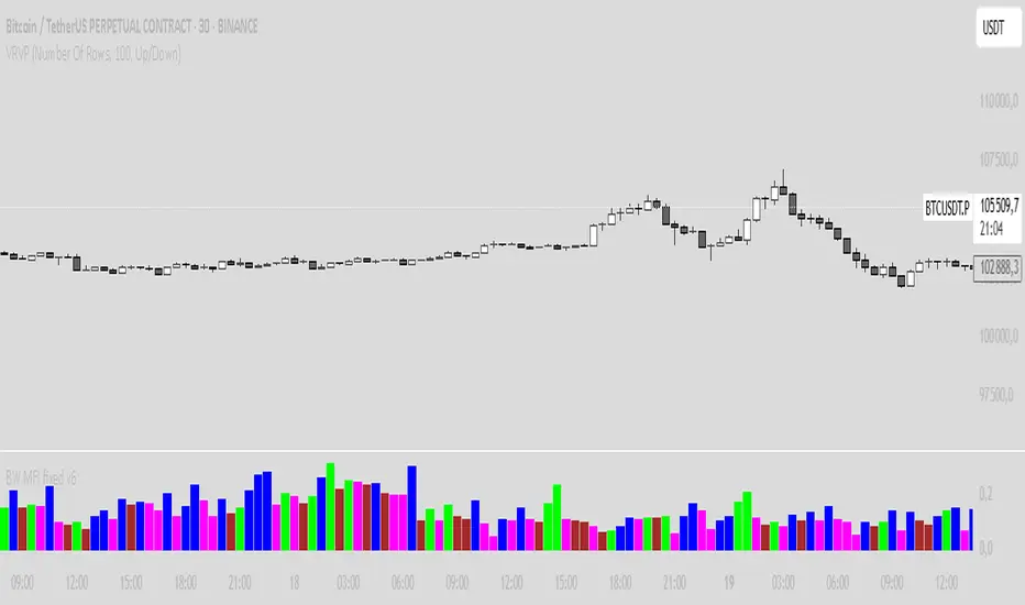
BW MFI fixed v6Bill Williams MFI
Sure! Here’s an English description of the indicator you have:
---
### Bill Williams Market Facilitation Index (MFI) — Indicator Description
This indicator implements the **Market Facilitation Index (MFI)** as introduced by Bill Williams. The MFI measures the market's willingness to move the price by comparing the price range to the volume.
---
### How it works:
* **MFI Calculation:**
The MFI is calculated as the difference between the current bar’s high and low prices divided by the volume of that bar:
$$
\text{MFI} = \frac{\text{High} - \text{Low}}{\text{Volume}}
$$
* **Color Coding Logic:**
The indicator compares the current MFI and volume values to their previous values and assigns colors to visualize market conditions according to Bill Williams’ methodology:
| Color | Condition | Market Interpretation |
| ----------- | ------------------ | --------------------------------------------------------------------------------------------- |
| **Green** | MFI ↑ and Volume ↑ | Strong trend continuation or acceleration (increased price movement supported by volume) |
| **Brown** | MFI ↓ and Volume ↓ | Trend weakening or possible pause (both price movement and volume are decreasing) |
| **Blue** | MFI ↑ and Volume ↓ | Possible false breakout or lack of conviction (price moves but volume decreases) |
| **Fuchsia** | MFI ↓ and Volume ↑ | Market indecision or battle between bulls and bears (volume rises but price movement shrinks) |
| **Gray** | None of the above | Neutral or unchanged market condition |
* **Display:**
The indicator plots the MFI values as colored columns on a separate pane below the price chart, providing a visual cue of the market’s behavior.
---
### Purpose:
This tool helps traders identify changes in market momentum and the strength behind price moves, providing insight into when trends might accelerate, weaken, or potentially reverse.
---
If you want, I can help you write a more detailed user guide or trading strategy based on this indicator!
COT IndexReference:
Trade Stocks and Commodities with the Insiders
Secrets of the COT Report by Larry Williams pg34
The equation is as below:
Current week's value- Lowest value of last three years
---------------------------------------------------------------------------- X 100%
Highest high of last three years-Lowest low of last three years
According to Larry Williams, traders should follow commercials direction. When the commercial index line (yellow line) is above 80, this indicates commercials are bullish. Hence, traders can look for potential buy setup. Conversely, when commercials index line (yellow line) is below 20, this indicates commercials are bearish, we can look for sell setup.
Do note that this is only applicable on Weekly chart as COT reports come out on weekly basis.
Modification from the original COT index from Larry Williams:
1) I've added 1year and 6months period, so traders maybe can look for pullback using shorter period. By default, Larry Williams uses 3 years Commercial index.
2) I've added non-commercials and retail traders index, they basically trade opposite way of commercials.
This indicator should not be used as a timing tool or entry tool, you can use it as your weekly or monthly bias tool. For more information, please read the books. Feel free to modify the code, if u have a better version of this, you may share to me if you want, I will be very grateful!

Student Wyckoff Target Shooter
**Target Shooter — Equal Move Target Tool (Larry Williams idea)**
**1. What this indicator does**
Target Shooter is a tool that measures the last meaningful price swing and projects an **equal move target** in the direction of the breakout.
The logic is simple:
* The market makes a move from point A to point B (a swing high to a swing low, or vice versa).
* Then price breaks out above or below this swing range.
* Target Shooter takes the size of that swing and **adds it in the direction of the breakout**, showing a logical **price target zone** where the move may:
* slow down,
* react,
* or potentially reverse.
This is a practical implementation of the “Equal Moves” idea often referenced by Larry Williams.
---
**2. Core idea (example)**
Example from the classic explanation:
* Price drops from **80 down to 20** → the move is **60 points**.
* The swing range is now: **High = 80, Low = 20**.
* Later, price **breaks above 80**.
Target Shooter assumes:
> “If the market could move 60 points in one direction, after a breakout it may travel another 60 points in the opposite direction.”
So the upside target becomes:
* Move size: 80 − 20 = 60
* Breakout above 80
* **Target = 80 + 60 = 140**
The indicator finds such swings automatically and draws:
* **UT (Upper Target)** on upside breakouts
* **DT (Down Target)** on downside breakouts
---
**3. What you see on the chart**
1. **Target lines**
* When price breaks **above** a previous swing range, the indicator plots a horizontal **UT (Upper Target)** line — the projected equal move target.
* When price breaks **below** the previous swing range, it plots a **DT (Down Target)** line — the downside target.
* Each line is drawn from the breakout bar and extended to the right for a user-defined number of bars.
2. **Price labels**
* A small label “UT” or “DT” is shown at the end of the line with the exact target price.
* This makes it easy to see where the projected target is without checking the scale.
3. **Optional swing range (debug view)**
* There is an option to display the **swing range** that the target is based on (similar to a Donchian channel on previous bars).
* This shows the upper (swing high) and lower (swing low) boundaries the indicator used to define the last move.
---
**4. Key inputs (plain language)**
* **Swing window length (bars)**
How many bars back the indicator looks to find the last meaningful swing (highest high and lowest low).
This is like the length of a Donchian channel used to define the previous range.
Smaller values → more frequent, shorter targets.
Larger values → bigger swings and more distant targets.
* **Minimum move size (in ticks)**
This is a noise filter.
If the distance between the swing high and swing low is smaller than this threshold, no targets are drawn.
The indicator will only react to moves that are big enough to matter for your trading.
* **Breakout type: Close vs High/Low**
* **Breakout by Close**:
The target appears only when the **bar closes** above/below the swing range.
More conservative and fewer false signals.
* **Breakout by High/Low**:
The target appears as soon as the **high** or **low** of the bar breaks the swing range.
Faster and more aggressive, but more sensitive to noise.
* **Target line length (bars)**
How far to the right the UT/DT lines should be extended.
Shorter length → local target zones.
Longer length → important levels visible far into the future.
* **Appearance settings**
* Separate color, width and style for **UT** and **DT** lines.
* Option to show or hide labels with price and “UT/DT” text.
---
**5. How to use Target Shooter in trading**
> Important: this is **not** an entry signal indicator.
> Target Shooter is a **targeting and context tool**, not a standalone system.
Typical uses:
1. **Planning take-profit zones**
* You already have an entry signal from your own strategy (Wyckoff, Larry Williams patterns, levels, volume, whatever you use).
* Target Shooter shows a **logical equal move target** where the current wave can reasonably “shoot”.
* You can:
* place your main take-profit around the target,
* scale out part of the position,
* tighten stops when price approaches the target.
2. **Finding potential reaction / reversal areas**
* Equal move targets often act as **zones of interest**.
* If price reaches a UT/DT level and then shows weakness/absorption/volume spikes or reversal candles, this might be a good place to take profits or look for counter-trend opportunities (for experienced traders).
3. **Assessing trend strength**
* If price **easily exceeds** the equal move target and keeps going without any reaction, it suggests a very strong trend.
* If price **fails to reach** the target and reverses early, the move is weaker than expected.
---
**6. Timeframes**
Target Shooter can be used on:
* **Intraday** (M5, M15, M30, H1) — for shorter-term targets within the day,
* **Higher timeframes** (H4, D1 and above) — for swing and position trades.
General rule:
The **higher the timeframe and the larger the swing**, the **more important** the target level tends to be.
---
**7. Notes and limitations**
* The indicator does **not** predict the future.
It simply projects a geometric equal move from the last swing.
* It should be combined with your own trading framework:
* support/resistance,
* Wyckoff / VSA,
* trend tools,
* volume/flow, etc.
* Always keep proper risk management.
A target is a **scenario**, not a guarantee.
.

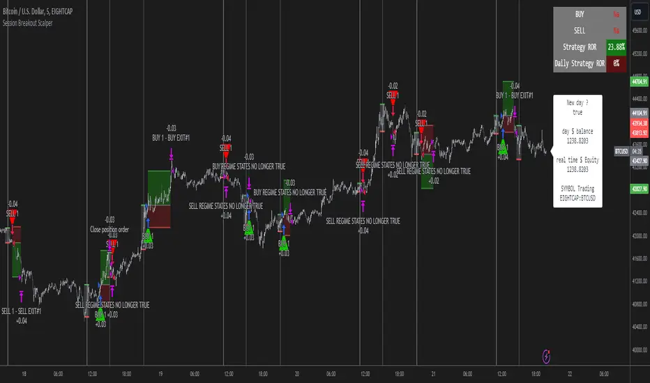
Session Breakout Scalper Trading BotHi Traders !
Introduction:
I have recently been exploring the world of automated algorithmic trading (as I prefer more objective trading strategies over subjective technical analysis (TA)) and would like to share one of my automation compatible (PineConnecter compatible) scripts “Session Breakout Scalper”.
The strategy is really simple and is based on time conditional breakouts although has more ”relatively” advanced optional features such as the regime indicators (Regime Filters) that attempt to filter out noise by adding more confluence states and the ATR multiple SL that takes into account volatility to mitigate the down side risk of the trade.
What is Algorthmic Trading:
Firstly what is algorithmic trading? Algorithmic trading also known as algo-trading, is a method of using computer programs (in this case pine script) to execute trades based on predetermined rules and instructions (this trading strategy). It's like having a robot trader who follows a strict set of commands to buy and sell assets automatically, without any human intervention.
Important Note:
For Algorithmic trading the strategy will require you having an essential TV subscription at the minimum (so that you can set alerts) plus a PineConnecter subscription (scroll down to the .”How does the strategy send signals” headings to read more)
The Strategy Explained:
Is the Time input true ? (this can be changed by toggling times under the “TRADE MEDIAN TIMES” group for user inputs).
Given the above is true the strategy waits x bars after the session and then calculates the highest high (HH) to lowest low (LL) range. For this box to form, the user defined amount of bars must print after the session. The box is symmetrical meaning the HH and LL are calculated over a lookback that is equal to the sum of user defined bars before and after the session (+ 1).
The Strategy then simultaneously defines the HH as the buy level (green line) and the LL as the sell level (red line). note the strategy will set stop orders at these levels respectively.
Enter a buy if price action crosses above the HH, and then cancel the sell order type (The opposite is true for a stop order).
If the momentum based regime filters are true the strategy will check for the regime / regimes to be true, if the regime if false the strategy will exit the current trade, as the regime filter has predicted a slowing / reversal of momentum.
The image below shows the strategy executing these trading rules ( Regime filters, "Trades on chart", "Signal & Label" and "Quantity" have been omitted. "Strategy label plots" has been switched to true)
Other Strategy Rules:
If a new session (time session which is user defined) is true (blue vertical line) and the strategy is currently still in a trade it will exit that trade immediately.
It is possible to also set a range of percentage gain per day that the strategy will try to acquire, if at any point the strategy’s profit is within the percentage range then the position / trade will be exited immediately (This can be changed in the “PERCENT DAY GAIN” group for user inputs)
Stops and Targets:
The strategy has either static (fixed) or variable SL options. TP however is only static. The “STRAT TP & TP” group of user inputs is responsible for the SL and TP values (quoted in pips). Note once the ATR stop is set to true the SL values in the above group no longer have any affect on the SL as expected.
What are the Regime Filters:
The Larry Williams Large Trade Index (LWLTI): The Larry Williams Large Trade Index (LWTI) is a momentum-based technical indicator developed by iconic trader Larry Williams. It identifies potential entries and exits for trades by gauging market sentiment, particularly the buying and selling pressure from large market players. Here's a breakdown of the LWTI:
LWLTI components and their interpretation:
Oscillator: It oscillates between 0 and 100, with 50 acting as the neutral line.
Sentiment Meter: Values above 75 suggest a bearish market dominated by large selling, while readings below 25 indicate a bullish market with strong buying from large players.
Trend Confirmation: Crossing above 75 during an uptrend and below 25 during a downtrend confirms the trend's continuation.
The Andean Oscillator (AO) : The Andean Oscillator is a trend and momentum based indicator designed to measure the degree of variations within individual uptrends and downtrends in the prices.
Regime Filter States:
In trading, a regime filter is a tool used to identify the current state or "regime" of the market.
These Regime filters are integrated within the trading strategy to attempt to lower risk (equity volatility and/or draw down). The regime filters have different states for each market order type (buy and sell). When the regime filters are set to true, if these regime states fail to be true the trade is exited immediately.
For Buy Trades:
LWLTI positive momentum state: Quotient of the lagged trailing difference and the ATR > 50
AO positive momentum state: Bull line > Bear line (signal line is omitted)
For Sell Trades:
LWLTI negative momentum stat: Quotient of the lagged trailing difference and the ATR < 50
AO negative momentum state: Bull line < Bear line (signal line is omitted)
How does the Strategy Send Signals:
The strategy triggers a TV alert (you will neet to set a alert first), TV then sends a HTTP request to the automation software (PineConnecter) which receives the request and then communicates to an MT4/5 EA to automate the trading strategy.
For the strategy to send signals you must have the following
At least a TV essential subscription
This Script added to your chart
A PineConnecter account, which is paid and not free. This will provide you with the expert advisor that executes trades based on these strategies signals.
For more detailed information on the automation process I would recommend you read the PineConnecter documentation and FAQ page.
Dashboard:
This Dashboard (top right by defualt) lists some simple trading statistics and also shows when a trade is live.
Important Notice:
- USE THIS STRATEGY AT YOUR OWN RISK AND ALWAYS DO YOUR OWN RESEARCH & MANUAL BACKTESTING !
- THE STRATEGY WILL NOT EXHIBIT THE BACKTEST PERFORMANCE SEEN BELOW IN ALL MARKETS !
Setup Max e Min Larry WilliansLarry Williams used this system to win the trading championship
Hello friends, I bring a script with a trading strategy to be used in futures such as Index, Forex and Commodities. Developed by famous trader Larry Williams.
In them we use two 3-period Simple Moving Averages (Arithmetic) (one with the high price, the other with the low price), and a 21-period Moving Average (Arithmetic) to determine the trend. This will form an average channel with the prices of the maximums and minimums of the last three candles.
Best time charts use the strategy: from 5 minutes to 60 minutes.
This strategy is quite simple. The 21 Moving Average will color according to the trend (Green for bullish, Red for bearish and Gray for transitions). The Script will signal the entry according to the trend by the colors of the candles and also by the signal:
When green, the buy will be on the crossing of the lower Moving Average crossing the candlestick, and the exit will be on the crossing of the candlestick on the next Upper Moving Average.
When red, the sell will be at the crossing of the Upper Moving Average crossing the candlestick, and the exit will be at the crossing of the candlestick on the next Lower Moving Average.
When the Script signals the candle with a purple X, it means that the trend is changing and the entire open operation must be closed.
This system has no Stop, so be careful when using it.
Na linguagem do autor:
Larry Williams usou esse sistema ganhar campeonato de trade
Olá amigos, trago um script com uma estratégia de trade pra ser usada em futuros como Índice, Forex e Commodities. Desenvolvido pelo famoso trader Larry Willians.
Neles usamos duas Médias Móveis Simples (Aritmética) de 3 períodos (uma com o preço da máxima, outra com o preço da mínima), e uma Média Móvel (Aritmética) de 21 períodos para determinar a tendência. Nisso vai formar uma canal de médias com os preços das máximas e mínimas dos últimos três candles.
Melhores tempos gráficos usar a estratégia: de 5 minutos até 60 minutos.
Essa estratégia é bem simples. A Média Móvel de 21 irá colorir de acordo com a tendência (Green pra alta, Red para baixa e Gray para transições). O Script irá sinalizar a entrada de acordo com a tendência pela cores dos candles e também pela sinalização:
Quando green, a compra será no cruzamento da Média Móvel inferior cruzando o candle, e a saida será no cruzamento do candle na Média Móvel Superior seguinte.
Quando red, a venda será no cruzamento da Média Móvel Superior cruzando o candle, e a saida será no cruzamento do candle na Média Móvel Inferior seguinte.
Quando o Script sinaliza o candle com X purple, significa que a tendência está em mudança e deve ser fechada toda a operação em aberto.
Este sistema não possui Stop, portando cuidado quanto a seu uso.

IndicatorsLibrary "Indicators"
cmf(lookback, n_to_smooth)
Calculates the Chaikin's Money Flow.
Parameters:
lookback (simple int)
n_to_smooth (simple int)
Returns: float The Money Flow value.
cmma(lookback, atr_length)
Calculates the CMMA (Close Minus Moving Average) indicator.
Parameters:
lookback (simple int)
atr_length (simple int)
Returns: float The CMMA value.
macd(fast_length, slow_length, n_to_smooth)
Calculates the normalized and scaled MACD.
Parameters:
fast_length (simple int)
slow_length (simple int)
n_to_smooth (simple int)
Returns: A tuple containing .
stochK(length, n_to_smooth)
Calculates a simplified Stochastic Oscillator.
Uses: 100 * ta.sma((close - lowest_low) / (highest_high - lowest_low), n_to_smooth)
Parameters:
length (simple int)
n_to_smooth (simple int)
Returns: float The Stochastic %K value.
williamsR(length)
Calculates the Williams %R using the stochK function.
Uses: -1 * (100 - stoch(length, 1))
Parameters:
length (simple int)
Returns: float The Williams %R value.

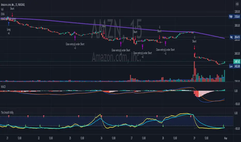
MACD Willy StrategyThis strategy is mainly developed for scalping / intraday trading. It could potentially be used to identify entry/exit signals for short term options trading. It performs decently well on popular stocks when used on time frames between 5 min to 15 min using regular session bar data. It combines 3 popular indicators, EMA, MACD, and William %range, to generate both long and short signals.
EMA:
Default is 200 EMA line.
MACD:
Default is 12/26 lengths for fast/slow signal inputs.
William %R - Smoothed (Published):
This is a custom indicator that generates two moving average lines from the original William %R line.
How it works:
Entry conditions:
1. Long/short entries when bar closes above/below EMA line
2. Long/short entries when MACD line is above/below signal line (histogram > 0 for long, < 0 for short)
3. Long/short entries when William %R fast MA line is above/below slow MA line
Exit conditions:
1. Exit long when MACD line is below signal line, vise versa for exit short
2. Exit long when William %R fast MA line is below slow MA line, vise versa for exit short
3. Exit long when William %R fast MA line must in below the overbought (-20) limit, exit short when above the oversold (-80) limit.
***Note that parameters are NOT optimized for any particular stocks / instruments.
Enjoy~~!!
100PipsADay third screen / triple screen strategy MACD and W%RThird Screen Strategy
This particular script is specifically designed around this strategy. D1 MACD & H1 Williams %.
I coded the script in a way that you automatically get the signal that is calculated taking in consideration both the indicators (macd and w%R)
Green means that the daily MACD histogram is above 0 (crowd is bullish) but w%R shows that momentarily there is a lower price (W%R is oversold),
Red is vice versa.
Quote from original post :
Below is how I would normally take a trade using my strategy.
As you can see below in my chart, I look on the D1 chart for the MACD to cross over.
Once it is clear that it has crossed over, I will enter positions on the H1 chart using Williams %.
end quote.
This Script i coded in a way that automatically account for both the indicators, so you don't have to switch between timeframes.
3 Important rules :
To get the indicator set correctly you need to use on 1 Hour time frame
-----------------------
You should wait 6 hours when signal appear to open an other position on the same pair
-----------------------
I coded an alarm that gets triggered when the pair meet both condition (when the bar and/or the background is green) so you can just set it by right clicking the indicator and be relaxed!
Italiano :
Strategia Third screen
Questo particolare script è specificamente progettato attorno a questa strategia. D1 MACD e H1 Williams%.
Ho codificato lo script in modo da ottenere automaticamente il segnale calcolato tenendo conto di entrambi gli indicatori (macd e w% R)
Verde indica che l'istogramma MACD giornaliero è superiore a 0 (la folla è rialzista) ma w% R mostra che momentaneamente esiste un prezzo inferiore (W% R è sotto il livello di oversold),
Il rosso è viceversa.
Ho codificato questo script in un modo che tiene conto automaticamente di entrambi gli indicatori, quindi non è necessario passare da un intervallo di tempo all'altro.
3 Regole importanti:
Per impostare correttamente l'indicatore è necessario utilizzare nel periodo di 1 ora
-----------------------
Dovresti aspettare 6 ore una volta che arriva il segnale per aprire un'altra posizione sullo stessa moneta
-----------------------
Ho codificato un allarme che viene attivato quando sono soddisfatte entrambe le condizioni (ossia quando lo sfondo è verde), quindi puoi semplicemente impostarlo facendo clic con il pulsante destro del mouse sull'indicatore ed essere rilassato!

$MTF Fractal Echo DetectorMIL:MTVFR FRACTAL ECHO DETECTOR by Timmy741
The first public multi-timeframe fractal convergence system that actually works.
Market makers don’t move price randomly.
They test the same fractal structure on lower timeframes first → then execute the real move on higher timeframes.
This indicator catches the “echo” — when 3–5 timeframes are printing fractals at almost the exact same price level.
That’s not coincidence. That’s preparation.
FEATURES
• 5 simultaneous timeframes (1min → 4H by default)
• Real Williams Fractal detection (configurable period)
• Dynamic echo tolerance & minimum TF alignment
• Visual S/R zones from every timeframe
• Bullish / Bearish echo convergence signals
• Strength meter (3/5, 4/5, 5/5 TF alignment)
• Zero repainting — uses proper lookahead=off
• Fully Pine v6 typed + optimized
USE CASE
When you see a 4/5 or 5/5 echo:
→ That level is being defended or attacked with intent
→ 80%+ chance the next real move comes from there
→ Trade the breakout or reversal at that exact fractal cluster
Works insane on:
• BTC / ETH (all timeframes)
• Nasdaq / SPX futures
• Forex majors (especially GBP & gold)
• 2025 small-cap rotation setups
100% Open Source • MPL 2.0 • Built by Timmy741 • December 2024
If you know about fractal echoes… you already know.
#fractal #mtf #echo #williamsfractal #multitimeframe #smartmoney #ict #smc #orderflow #convergence #timmy741 #snr #structure

Profitunity - Beginner [TC]This indicator aggregates the knowledges of the first level of the Trading Chaos approach by Bill Williams. It uses the Market Facilitation Index (MFI) in conjunction with the type of bar(candle) to generate strong long and strong short signals.
General information
Bars numeration
All bars or candles could be numbered with the following algorithm. If we divide the candle for 3 equal parts from high to low. The highest third have the number 1, the middle one - 2, the lowest one - 3. Hence we can define the first number as the number of the third where the price opened, second - where the price closed. For example, if the price opened at the highest third and closed at the lowest one this candle has the number 13.
Trend defining
Also candles could be divided into three groups according to the trend condition: uptrend, downtrend, sideways. If the middle of the candle's trading range is above the high of the previous candle - it's uptrend candle, if below the low of the previous candle - it's downtrend candle, sideways in other candles.
Profitunity windows
According to Bill Williams MFI has 4 windows - fake, green, fade and squat. I am not going to describe here the methodology of MFI, but one thing you should know that the most valuable windows are green and squat. Green state is an indication of the true move on the market. Squat the sign that the increase in volume have not triggered the trend continuation and reverse is about to happen.
How to use?
You can use this script as the helper in automatic defining the type of candle. Indicator shows only green (green candle color) and squat (red candle color) MFI states. Add script to any timeframe and asset chart to see labels.
The "strong long" label flashes when 3 conditions are met:
1. Squat candle
2. Candle number 13
3. Downtrend candle
"Strong short" label flashes when:
1. Squat candle
2. Candle number 31
3. Uptrend candle
This indicator helps to find the trend reversal points, can be used in conjunction with other TA tools to find the entry points.

taLibrary "ta"
█ OVERVIEW
This library holds technical analysis functions calculating values for which no Pine built-in exists.
Look first. Then leap.
█ FUNCTIONS
cagr(entryTime, entryPrice, exitTime, exitPrice)
It calculates the "Compound Annual Growth Rate" between two points in time. The CAGR is a notional, annualized growth rate that assumes all profits are reinvested. It only takes into account the prices of the two end points — not drawdowns, so it does not calculate risk. It can be used as a yardstick to compare the performance of two instruments. Because it annualizes values, the function requires a minimum of one day between the two end points (annualizing returns over smaller periods of times doesn't produce very meaningful figures).
Parameters:
entryTime : The starting timestamp.
entryPrice : The starting point's price.
exitTime : The ending timestamp.
exitPrice : The ending point's price.
Returns: CAGR in % (50 is 50%). Returns `na` if there is not >=1D between `entryTime` and `exitTime`, or until the two time points have not been reached by the script.
█ v2, Mar. 8, 2022
Added functions `allTimeHigh()` and `allTimeLow()` to find the highest or lowest value of a source from the first historical bar to the current bar. These functions will not look ahead; they will only return new highs/lows on the bar where they occur.
allTimeHigh(src)
Tracks the highest value of `src` from the first historical bar to the current bar.
Parameters:
src : (series int/float) Series to track. Optional. The default is `high`.
Returns: (float) The highest value tracked.
allTimeLow(src)
Tracks the lowest value of `src` from the first historical bar to the current bar.
Parameters:
src : (series int/float) Series to track. Optional. The default is `low`.
Returns: (float) The lowest value tracked.
█ v3, Sept. 27, 2022
This version includes the following new functions:
aroon(length)
Calculates the values of the Aroon indicator.
Parameters:
length (simple int) : (simple int) Number of bars (length).
Returns: ( [float, float ]) A tuple of the Aroon-Up and Aroon-Down values.
coppock(source, longLength, shortLength, smoothLength)
Calculates the value of the Coppock Curve indicator.
Parameters:
source (float) : (series int/float) Series of values to process.
longLength (simple int) : (simple int) Number of bars for the fast ROC value (length).
shortLength (simple int) : (simple int) Number of bars for the slow ROC value (length).
smoothLength (simple int) : (simple int) Number of bars for the weigted moving average value (length).
Returns: (float) The oscillator value.
dema(source, length)
Calculates the value of the Double Exponential Moving Average (DEMA).
Parameters:
source (float) : (series int/float) Series of values to process.
length (simple int) : (simple int) Length for the smoothing parameter calculation.
Returns: (float) The double exponentially weighted moving average of the `source`.
dema2(src, length)
An alternate Double Exponential Moving Average (Dema) function to `dema()`, which allows a "series float" length argument.
Parameters:
src : (series int/float) Series of values to process.
length : (series int/float) Length for the smoothing parameter calculation.
Returns: (float) The double exponentially weighted moving average of the `src`.
dm(length)
Calculates the value of the "Demarker" indicator.
Parameters:
length (simple int) : (simple int) Number of bars (length).
Returns: (float) The oscillator value.
donchian(length)
Calculates the values of a Donchian Channel using `high` and `low` over a given `length`.
Parameters:
length (int) : (series int) Number of bars (length).
Returns: ( [float, float, float ]) A tuple containing the channel high, low, and median, respectively.
ema2(src, length)
An alternate ema function to the `ta.ema()` built-in, which allows a "series float" length argument.
Parameters:
src : (series int/float) Series of values to process.
length : (series int/float) Number of bars (length).
Returns: (float) The exponentially weighted moving average of the `src`.
eom(length, div)
Calculates the value of the Ease of Movement indicator.
Parameters:
length (simple int) : (simple int) Number of bars (length).
div (simple int) : (simple int) Divisor used for normalzing values. Optional. The default is 10000.
Returns: (float) The oscillator value.
frama(source, length)
The Fractal Adaptive Moving Average (FRAMA), developed by John Ehlers, is an adaptive moving average that dynamically adjusts its lookback period based on fractal geometry.
Parameters:
source (float) : (series int/float) Series of values to process.
length (int) : (series int) Number of bars (length).
Returns: (float) The fractal adaptive moving average of the `source`.
ft(source, length)
Calculates the value of the Fisher Transform indicator.
Parameters:
source (float) : (series int/float) Series of values to process.
length (simple int) : (simple int) Number of bars (length).
Returns: (float) The oscillator value.
ht(source)
Calculates the value of the Hilbert Transform indicator.
Parameters:
source (float) : (series int/float) Series of values to process.
Returns: (float) The oscillator value.
ichimoku(conLength, baseLength, senkouLength)
Calculates values of the Ichimoku Cloud indicator, including tenkan, kijun, senkouSpan1, senkouSpan2, and chikou. NOTE: offsets forward or backward can be done using the `offset` argument in `plot()`.
Parameters:
conLength (int) : (series int) Length for the Conversion Line (Tenkan). The default is 9 periods, which returns the mid-point of the 9 period Donchian Channel.
baseLength (int) : (series int) Length for the Base Line (Kijun-sen). The default is 26 periods, which returns the mid-point of the 26 period Donchian Channel.
senkouLength (int) : (series int) Length for the Senkou Span 2 (Leading Span B). The default is 52 periods, which returns the mid-point of the 52 period Donchian Channel.
Returns: ( [float, float, float, float, float ]) A tuple of the Tenkan, Kijun, Senkou Span 1, Senkou Span 2, and Chikou Span values. NOTE: by default, the senkouSpan1 and senkouSpan2 should be plotted 26 periods in the future, and the Chikou Span plotted 26 days in the past.
ift(source)
Calculates the value of the Inverse Fisher Transform indicator.
Parameters:
source (float) : (series int/float) Series of values to process.
Returns: (float) The oscillator value.
kvo(fastLen, slowLen, trigLen)
Calculates the values of the Klinger Volume Oscillator.
Parameters:
fastLen (simple int) : (simple int) Length for the fast moving average smoothing parameter calculation.
slowLen (simple int) : (simple int) Length for the slow moving average smoothing parameter calculation.
trigLen (simple int) : (simple int) Length for the trigger moving average smoothing parameter calculation.
Returns: ( [float, float ]) A tuple of the KVO value, and the trigger value.
pzo(length)
Calculates the value of the Price Zone Oscillator.
Parameters:
length (simple int) : (simple int) Length for the smoothing parameter calculation.
Returns: (float) The oscillator value.
rms(source, length)
Calculates the Root Mean Square of the `source` over the `length`.
Parameters:
source (float) : (series int/float) Series of values to process.
length (int) : (series int) Number of bars (length).
Returns: (float) The RMS value.
rwi(length)
Calculates the values of the Random Walk Index.
Parameters:
length (simple int) : (simple int) Lookback and ATR smoothing parameter length.
Returns: ( [float, float ]) A tuple of the `rwiHigh` and `rwiLow` values.
stc(source, fast, slow, cycle, d1, d2)
Calculates the value of the Schaff Trend Cycle indicator.
Parameters:
source (float) : (series int/float) Series of values to process.
fast (simple int) : (simple int) Length for the MACD fast smoothing parameter calculation.
slow (simple int) : (simple int) Length for the MACD slow smoothing parameter calculation.
cycle (simple int) : (simple int) Number of bars for the Stochastic values (length).
d1 (simple int) : (simple int) Length for the initial %D smoothing parameter calculation.
d2 (simple int) : (simple int) Length for the final %D smoothing parameter calculation.
Returns: (float) The oscillator value.
stochFull(periodK, smoothK, periodD)
Calculates the %K and %D values of the Full Stochastic indicator.
Parameters:
periodK (simple int) : (simple int) Number of bars for Stochastic calculation. (length).
smoothK (simple int) : (simple int) Number of bars for smoothing of the %K value (length).
periodD (simple int) : (simple int) Number of bars for smoothing of the %D value (length).
Returns: ( [float, float ]) A tuple of the slow %K and the %D moving average values.
stochRsi(lengthRsi, periodK, smoothK, periodD, source)
Calculates the %K and %D values of the Stochastic RSI indicator.
Parameters:
lengthRsi (simple int) : (simple int) Length for the RSI smoothing parameter calculation.
periodK (simple int) : (simple int) Number of bars for Stochastic calculation. (length).
smoothK (simple int) : (simple int) Number of bars for smoothing of the %K value (length).
periodD (simple int) : (simple int) Number of bars for smoothing of the %D value (length).
source (float) : (series int/float) Series of values to process. Optional. The default is `close`.
Returns: ( [float, float ]) A tuple of the slow %K and the %D moving average values.
supertrend(factor, atrLength, wicks)
Calculates the values of the SuperTrend indicator with the ability to take candle wicks into account, rather than only the closing price.
Parameters:
factor (float) : (series int/float) Multiplier for the ATR value.
atrLength (simple int) : (simple int) Length for the ATR smoothing parameter calculation.
wicks (simple bool) : (simple bool) Condition to determine whether to take candle wicks into account when reversing trend, or to use the close price. Optional. Default is false.
Returns: ( [float, int ]) A tuple of the superTrend value and trend direction.
szo(source, length)
Calculates the value of the Sentiment Zone Oscillator.
Parameters:
source (float) : (series int/float) Series of values to process.
length (simple int) : (simple int) Length for the smoothing parameter calculation.
Returns: (float) The oscillator value.
t3(source, length, vf)
Calculates the value of the Tilson Moving Average (T3).
Parameters:
source (float) : (series int/float) Series of values to process.
length (simple int) : (simple int) Length for the smoothing parameter calculation.
vf (simple float) : (simple float) Volume factor. Affects the responsiveness.
Returns: (float) The Tilson moving average of the `source`.
t3Alt(source, length, vf)
An alternate Tilson Moving Average (T3) function to `t3()`, which allows a "series float" `length` argument.
Parameters:
source (float) : (series int/float) Series of values to process.
length (float) : (series int/float) Length for the smoothing parameter calculation.
vf (simple float) : (simple float) Volume factor. Affects the responsiveness.
Returns: (float) The Tilson moving average of the `source`.
tema(source, length)
Calculates the value of the Triple Exponential Moving Average (TEMA).
Parameters:
source (float) : (series int/float) Series of values to process.
length (simple int) : (simple int) Length for the smoothing parameter calculation.
Returns: (float) The triple exponentially weighted moving average of the `source`.
tema2(source, length)
An alternate Triple Exponential Moving Average (TEMA) function to `tema()`, which allows a "series float" `length` argument.
Parameters:
source (float) : (series int/float) Series of values to process.
length (float) : (series int/float) Length for the smoothing parameter calculation.
Returns: (float) The triple exponentially weighted moving average of the `source`.
trima(source, length)
Calculates the value of the Triangular Moving Average (TRIMA).
Parameters:
source (float) : (series int/float) Series of values to process.
length (int) : (series int) Number of bars (length).
Returns: (float) The triangular moving average of the `source`.
trima2(src, length)
An alternate Triangular Moving Average (TRIMA) function to `trima()`, which allows a "series int" length argument.
Parameters:
src : (series int/float) Series of values to process.
length : (series int) Number of bars (length).
Returns: (float) The triangular moving average of the `src`.
trix(source, length, signalLength, exponential)
Calculates the values of the TRIX indicator.
Parameters:
source (float) : (series int/float) Series of values to process.
length (simple int) : (simple int) Length for the smoothing parameter calculation.
signalLength (simple int) : (simple int) Length for smoothing the signal line.
exponential (simple bool) : (simple bool) Condition to determine whether exponential or simple smoothing is used. Optional. The default is `true` (exponential smoothing).
Returns: ( [float, float, float ]) A tuple of the TRIX value, the signal value, and the histogram.
uo(fastLen, midLen, slowLen)
Calculates the value of the Ultimate Oscillator.
Parameters:
fastLen (simple int) : (series int) Number of bars for the fast smoothing average (length).
midLen (simple int) : (series int) Number of bars for the middle smoothing average (length).
slowLen (simple int) : (series int) Number of bars for the slow smoothing average (length).
Returns: (float) The oscillator value.
vhf(source, length)
Calculates the value of the Vertical Horizontal Filter.
Parameters:
source (float) : (series int/float) Series of values to process.
length (simple int) : (simple int) Number of bars (length).
Returns: (float) The oscillator value.
vi(length)
Calculates the values of the Vortex Indicator.
Parameters:
length (simple int) : (simple int) Number of bars (length).
Returns: ( [float, float ]) A tuple of the viPlus and viMinus values.
vzo(length)
Calculates the value of the Volume Zone Oscillator.
Parameters:
length (simple int) : (simple int) Length for the smoothing parameter calculation.
Returns: (float) The oscillator value.
williamsFractal(period)
Detects Williams Fractals.
Parameters:
period (int) : (series int) Number of bars (length).
Returns: ( [bool, bool ]) A tuple of an up fractal and down fractal. Variables are true when detected.
wpo(length)
Calculates the value of the Wave Period Oscillator.
Parameters:
length (simple int) : (simple int) Length for the smoothing parameter calculation.
Returns: (float) The oscillator value.
█ v7, Nov. 2, 2023
This version includes the following new and updated functions:
atr2(length)
An alternate ATR function to the `ta.atr()` built-in, which allows a "series float" `length` argument.
Parameters:
length (float) : (series int/float) Length for the smoothing parameter calculation.
Returns: (float) The ATR value.
changePercent(newValue, oldValue)
Calculates the percentage difference between two distinct values.
Parameters:
newValue (float) : (series int/float) The current value.
oldValue (float) : (series int/float) The previous value.
Returns: (float) The percentage change from the `oldValue` to the `newValue`.
donchian(length)
Calculates the values of a Donchian Channel using `high` and `low` over a given `length`.
Parameters:
length (int) : (series int) Number of bars (length).
Returns: ( [float, float, float ]) A tuple containing the channel high, low, and median, respectively.
highestSince(cond, source)
Tracks the highest value of a series since the last occurrence of a condition.
Parameters:
cond (bool) : (series bool) A condition which, when `true`, resets the tracking of the highest `source`.
source (float) : (series int/float) Series of values to process. Optional. The default is `high`.
Returns: (float) The highest `source` value since the last time the `cond` was `true`.
lowestSince(cond, source)
Tracks the lowest value of a series since the last occurrence of a condition.
Parameters:
cond (bool) : (series bool) A condition which, when `true`, resets the tracking of the lowest `source`.
source (float) : (series int/float) Series of values to process. Optional. The default is `low`.
Returns: (float) The lowest `source` value since the last time the `cond` was `true`.
relativeVolume(length, anchorTimeframe, isCumulative, adjustRealtime)
Calculates the volume since the last change in the time value from the `anchorTimeframe`, the historical average volume using bars from past periods that have the same relative time offset as the current bar from the start of its period, and the ratio of these volumes. The volume values are cumulative by default, but can be adjusted to non-accumulated with the `isCumulative` parameter.
Parameters:
length (simple int) : (simple int) The number of periods to use for the historical average calculation.
anchorTimeframe (simple string) : (simple string) The anchor timeframe used in the calculation. Optional. Default is "D".
isCumulative (simple bool) : (simple bool) If `true`, the volume values will be accumulated since the start of the last `anchorTimeframe`. If `false`, values will be used without accumulation. Optional. The default is `true`.
adjustRealtime (simple bool) : (simple bool) If `true`, estimates the cumulative value on unclosed bars based on the data since the last `anchor` condition. Optional. The default is `false`.
Returns: ( [float, float, float ]) A tuple of three float values. The first element is the current volume. The second is the average of volumes at equivalent time offsets from past anchors over the specified number of periods. The third is the ratio of the current volume to the historical average volume.
rma2(source, length)
An alternate RMA function to the `ta.rma()` built-in, which allows a "series float" `length` argument.
Parameters:
source (float) : (series int/float) Series of values to process.
length (float) : (series int/float) Length for the smoothing parameter calculation.
Returns: (float) The rolling moving average of the `source`.
supertrend2(factor, atrLength, wicks)
An alternate SuperTrend function to `supertrend()`, which allows a "series float" `atrLength` argument.
Parameters:
factor (float) : (series int/float) Multiplier for the ATR value.
atrLength (float) : (series int/float) Length for the ATR smoothing parameter calculation.
wicks (simple bool) : (simple bool) Condition to determine whether to take candle wicks into account when reversing trend, or to use the close price. Optional. Default is `false`.
Returns: ( [float, int ]) A tuple of the superTrend value and trend direction.
vStop(source, atrLength, atrFactor)
Calculates an ATR-based stop value that trails behind the `source`. Can serve as a possible stop-loss guide and trend identifier.
Parameters:
source (float) : (series int/float) Series of values that the stop trails behind.
atrLength (simple int) : (simple int) Length for the ATR smoothing parameter calculation.
atrFactor (float) : (series int/float) The multiplier of the ATR value. Affects the maximum distance between the stop and the `source` value. A value of 1 means the maximum distance is 100% of the ATR value. Optional. The default is 1.
Returns: ( [float, bool ]) A tuple of the volatility stop value and the trend direction as a "bool".
vStop2(source, atrLength, atrFactor)
An alternate Volatility Stop function to `vStop()`, which allows a "series float" `atrLength` argument.
Parameters:
source (float) : (series int/float) Series of values that the stop trails behind.
atrLength (float) : (series int/float) Length for the ATR smoothing parameter calculation.
atrFactor (float) : (series int/float) The multiplier of the ATR value. Affects the maximum distance between the stop and the `source` value. A value of 1 means the maximum distance is 100% of the ATR value. Optional. The default is 1.
Returns: ( [float, bool ]) A tuple of the volatility stop value and the trend direction as a "bool".
Removed Functions:
allTimeHigh(src)
Tracks the highest value of `src` from the first historical bar to the current bar.
allTimeLow(src)
Tracks the lowest value of `src` from the first historical bar to the current bar.
trima2(src, length)
An alternate Triangular Moving Average (TRIMA) function to `trima()`, which allows a
"series int" length argument.

Mean Reversion Oscillator [Alpha Extract]An advanced composite oscillator system specifically designed to identify extreme market conditions and high-probability mean reversion opportunities, combining five proven oscillators into a single, powerful analytical framework.
By integrating multiple momentum and volume-based indicators with sophisticated extreme level detection, this oscillator provides precise entry signals for contrarian trading strategies while filtering out false reversals through momentum confirmation.
🔶 Multi-Oscillator Composite Framework
Utilizes a comprehensive approach that combines Bollinger %B, RSI, Stochastic, Money Flow Index, and Williams %R into a unified composite score. This multi-dimensional analysis ensures robust signal generation by capturing different aspects of market extremes and momentum shifts.
// Weighted composite (equal weights)
normalized_bb = bb_percent
normalized_rsi = rsi
normalized_stoch = stoch_d_val
normalized_mfi = mfi
normalized_williams = williams_r
composite_raw = (normalized_bb + normalized_rsi + normalized_stoch + normalized_mfi + normalized_williams) / 5
composite = ta.sma(composite_raw, composite_smooth)
🔶 Advanced Extreme Level Detection
Features a sophisticated dual-threshold system that distinguishes between moderate and extreme market conditions. This hierarchical approach allows traders to identify varying degrees of mean reversion potential, from moderate oversold/overbought conditions to extreme levels that demand immediate attention.
🔶 Momentum Confirmation System
Incorporates a specialized momentum histogram that confirms mean reversion signals by analyzing the rate of change in the composite oscillator. This prevents premature entries during strong trending conditions while highlighting genuine reversal opportunities.
// Oscillator momentum (rate of change)
osc_momentum = ta.mom(composite, 5)
histogram = osc_momentum
// Momentum confirmation
momentum_bullish = histogram > histogram
momentum_bearish = histogram < histogram
// Confirmed signals
confirmed_bullish = bullish_entry and momentum_bullish
confirmed_bearish = bearish_entry and momentum_bearish
🔶 Dynamic Visual Intelligence
The oscillator line adapts its color intensity based on proximity to extreme levels, providing instant visual feedback about market conditions. Background shading creates clear zones that highlight when markets enter moderate or extreme territories.
🔶 Intelligent Signal Generation
Generates precise entry signals only when the composite oscillator crosses extreme thresholds with momentum confirmation. This dual-confirmation approach significantly reduces false signals while maintaining sensitivity to genuine mean reversion opportunities.
How It Works
🔶 Composite Score Calculation
The indicator simultaneously tracks five different oscillators, each normalized to a 0-100 scale, then combines them into a smoothed composite score. This approach eliminates the noise inherent in single-oscillator analysis while capturing the consensus view of multiple momentum indicators.
// Mean reversion entry signals
bullish_entry = ta.crossover(composite, 100 - extreme_level) and composite < (100 - extreme_level)
bearish_entry = ta.crossunder(composite, extreme_level) and composite > extreme_level
// Bollinger %B calculation
bb_basis = ta.sma(src, bb_length)
bb_dev = bb_mult * ta.stdev(src, bb_length)
bb_percent = (src - bb_lower) / (bb_upper - bb_lower) * 100
🔶 Extreme Zone Identification
The system automatically identifies when markets reach statistically significant extreme levels, both moderate (65/35) and extreme (80/20). These zones represent areas where mean reversion has the highest probability of success based on historical market behavior.
🔶 Momentum Histogram Analysis
A specialized momentum histogram tracks the velocity of oscillator changes, helping traders distinguish between healthy corrections and potential trend reversals. The histogram's color-coded display makes momentum shifts immediately apparent.
🔶 Divergence Detection Framework
Built-in divergence analysis identifies situations where price and oscillator movements diverge, often signaling impending reversals. Diamond-shaped markers highlight these critical divergence patterns for enhanced pattern recognition.
🔶 Real-Time Information Dashboard
An integrated information table provides instant access to current oscillator readings, market status, and individual component values. This dashboard eliminates the need to manually check multiple indicators while trading.
🔶 Individual Component Display
Optional display of individual oscillator components allows traders to understand which specific indicators are driving the composite signal. This transparency enables more informed decision-making and deeper market analysis.
🔶 Adaptive Background Coloring
Intelligent background shading automatically adjusts based on market conditions, creating visual zones that correspond to different levels of mean reversion potential. The subtle color gradations make pattern recognition effortless.
1D
3D
🔶 Comprehensive Alert System
Multi-tier alert system covers confirmed entry signals, divergence patterns, and extreme level breaches. Each alert type provides specific context about the detected condition, enabling traders to respond appropriately to different signal strengths.
🔶 Customizable Threshold Management
Fully adjustable extreme and moderate levels allow traders to fine-tune the indicator's sensitivity to match different market volatilities and trading timeframes. This flexibility ensures optimal performance across various market conditions.
🔶 Why Choose AE - Mean Reversion Oscillator?
This indicator provides the most comprehensive approach to mean reversion trading by combining multiple proven oscillators with advanced confirmation mechanisms. By offering clear visual hierarchies for different extreme levels and requiring momentum confirmation for signals, it empowers traders to identify high-probability contrarian opportunities while avoiding false reversals. The sophisticated composite methodology ensures that signals are both statistically significant and practically actionable, making it an essential tool for traders focused on mean reversion strategies across all market conditions.