Price Action Smart Money Concepts [BigBeluga]THE SMART MONEY CONCEPTS Toolkit
The Smart Money Concepts [ BigBeluga ] is a comprehensive toolkit built around the principles of "smart money" behavior, which refers to the actions and strategies of institutional investors.
The Smart Money Concepts Toolkit brings together a suite of advanced indicators that are all interconnected and built around a unified concept: understanding and trading like institutional investors, or "smart money." These indicators are not just randomly chosen tools; they are features of a single overarching framework, which is why having them all in one place creates such a powerful system.
This all-in-one toolkit provides the user with a unique experience by automating most of the basic and advanced concepts on the chart, saving them time and improving their trading ideas.
Real-time market structure analysis simplifies complex trends by pinpointing key support, resistance, and breakout levels.
Advanced order block analysis leverages detailed volume data to pinpoint high-demand zones, revealing internal market sentiment and predicting potential reversals. This analysis utilizes bid/ask zones to provide supply/demand insights, empowering informed trading decisions.
Imbalance Concepts (FVG and Breakers) allows traders to identify potential market weaknesses and areas where price might be attracted to fill the gap, creating opportunities for entry and exit.
Swing failure patterns help traders identify potential entry points and rejection zones based on price swings.
Liquidity Concepts, our advanced liquidity algorithm, pinpoints high-impact events, allowing you to predict market shifts, strong price reactions, and potential stop-loss hunting zones. This gives traders an edge to make informed trading decisions based on liquidity dynamics.
🔵 FEATURES
The indicator has quite a lot of features that are provided below:
Swing market structure
Internal market structure
Mapping structure
Adjustable market structure
Strong/Weak H&L
Sweep
Volumetric Order block / Breakers
Fair Value Gaps / Breakers (multi-timeframe)
Swing Failure Patterns (multi-timeframe)
Deviation area
Equal H&L
Liquidity Prints
Buyside & Sellside
Sweep Area
Highs and Lows (multi-timeframe)
🔵 BASIC DEMONSTRATION OF ALL FEATURES
1. MARKET STRUCTURE
The preceding image illustrates the market structure functionality within the Smart Money Concepts indicator.
➤ Solid lines: These represent the core indicator's internal structure, forming the foundation for most other components. They visually depict the overall market direction and identify major reversal points marked by significant price movements (denoted as 'x').
➤ Internal Structure: These represent an alternative internal structure with the potential to drive more rapid market shifts. This is particularly relevant when a significant gap exists in the established swing structure, specifically between the Break of Structure (BOS) and the most recent Change of High/Low (CHoCH). Identifying these formations can offer opportunities for quicker entries and potential short-term reversals.
➤ Sweeps (x): These signify potential turning points in the market where liquidity is removed from the structure. This suggests a possible trend reversal and presents crucial entry opportunities. Sweeps are identified within both swing and internal structures, providing valuable insights for informed trading decisions.
➤ Mapping structure: A tool that automatically identifies and connects significant price highs and lows, creating a zig-zag pattern. It visualizes market structure, highlights trends, support/resistance levels, and potential breakouts. Helps traders quickly grasp price action patterns and make informed decisions.
➤ Color-coded candles based on market structure: These colors visually represent the underlying market structure, making it easier for traders to quickly identify trends.
➤ Extreme H&L: It visualizes market structure with extreme high and lows, which gives perspective for macro Market Structure.
2. VOLUMETRIC ORDER BLOCKS
Order blocks are specific areas on a financial chart where significant buying or selling activity has occurred. These are not just simple zones; they contain valuable information about market dynamics. Within each of these order blocks, volume bars represent the actual buying and selling activity that took place. These volume bars offer deeper insights into the strength of the order block by showing how much buying or selling power is concentrated in that specific zone.
Additionally, these order blocks can be transformed into Breaker Blocks. When an order block fails—meaning the price breaks through this zone without reversing—it becomes a breaker block. Breaker blocks are particularly useful for trading breakouts, as they signal that the market has shifted beyond a previously established zone, offering opportunities for traders to enter in the direction of the breakout.
Here's a breakdown:
➤ Bear Order Blocks (Red): These are zones where a lot of selling happened. Traders see these areas as places where sellers were strong, pushing the price down. When the price returns to these zones, it might face resistance and drop again.
➤ Bull Order Blocks (Green): These are zones where a lot of buying happened. Traders see these areas as places where buyers were strong, pushing the price up. When the price returns to these zones, it might find support and rise again.
These Order Blocks help traders identify potential areas for entering or exiting trades based on past market activity. The volume bars inside blocks show the amount of trading activity that occurred in these blocks, giving an idea of the strength of buying or selling pressure.
➤ Breaker Block: When an order block fails, meaning the price breaks through this zone without reversing, it becomes a breaker block. This indicates a significant shift in market liquidity and structure.
➤ A bearish breaker block occurs after a bullish order block fails. This typically happens when there's an upward trend, and a certain level that was expected to support the market's rise instead gives way, leading to a sharp decline. This decline indicates that sellers have overcome the buyers, absorbing liquidity and shifting the sentiment from bullish to bearish.
Conversely, a bullish breaker block is formed from the failure of a bearish order block. In a downtrend, when a level that was expected to act as resistance is breached, and the price shoots up, it signifies that buyers have taken control, overpowering the sellers.
3. FAIR VALUE GAPS:
A fair value gap (FVG), also referred to as an imbalance, is an essential concept in Smart Money trading. It highlights the supply and demand dynamics. This gap arises when there's a notable difference between the volume of buy and sell orders. FVGs can be found across various asset classes, including forex, commodities, stocks, and cryptocurrencies.
FVGs in this toolkit have the ability to detect raids of FVG which helps to identify potential price reversals.
Mitigation option helps to change from what source FVGs will be identified: Close, Wicks or AVG.
4. SWING FAILURE PATTERN (SFP):
The Swing Failure Pattern is a liquidity engineering pattern, generally used to fill large orders. This means, the SFP generally occurs when larger players push the price into liquidity pockets with the sole objective of filling their own positions.
SFP is a technical analysis tool designed to identify potential market reversals. It works by detecting instances where the price briefly breaks a previous high or low but fails to maintain that breakout, quickly reversing direction.
How it works:
Pattern Detection: The indicator scans for price movements that breach recent highs or lows.
Reversal Confirmation: If the price quickly reverses after breaching these levels, it's identified as an SFP.
➤ SFP Display:
Bullish SFP: Marked with a green symbol when price drops below a recent low before reversing upwards.
Bearish SFP: Marked with a red symbol when price rises above a recent high before reversing downwards.
➤ Deviation Levels: After detecting an SFP, the indicator projects white lines showing potential price deviation:
For bullish SFPs, the deviation line appears above the current price.
For bearish SFPs, the deviation line appears below the current price.
These deviation levels can serve as a potential trading opportunity or areas where the reversal might lose momentum.
With Volume Threshold and Filtering of SFP traders can adjust their trading style:
Volume Threshold: This setting allows traders to filter SFPs based on the volume of the reversal candle. By setting a higher volume threshold, traders can focus on potentially more significant reversals that are backed by higher trading activity.
SFP Filtering: This feature enables traders to filter SFP detection. It includes parameters such as:
5. LIQUIDITY CONCEPTS:
➤ Equal Lows (EQL) and Equal Highs (EQH) are important concepts in liquidity-based trading.
EQL: A series of two or more swing lows that occur at approximately the same price level.
EQH: A series of two or more swing highs that occur at approximately the same price level.
EQLs and EQHs are seen as potential liquidity pools where a large number of stop loss orders or limit orders may be clustered. They can be used as potential reverse points for trades.
This multi-period feature allows traders to select less and more significant EQL and EQH:
➤ Liquidity wicks:
Liquidity wicks are a minor representation of a stop-loss hunt during the retracement of a pivot point:
➤ Buy and Sell side liquidity:
The buy side liquidity represents a concentration of potential buy orders below the current price level. When price moves into this area, it can lead to increased buying pressure due to the execution of these orders.
The sell side liquidity indicates a pool of potential sell orders below the current price level. Price movement into this area can result in increased selling pressure as these orders are executed.
➤ Sweep Liquidation Zones:
Sweep Liquidation Zones are crucial for understanding market structure and potential future price movements. They provide insights into areas where significant market participants have been forced out of their positions, potentially setting up new trading opportunities.
🔵 USAGE & EXAMPLES
The core principle behind the success of this toolkit lies in identifying "confluence." This refers to the convergence of multiple trading indicators all signaling the same information at a specific point or area. By seeking such alignment, traders can significantly enhance the likelihood of successful trades.
MS + OBs
The chart illustrates a highly bullish setup where the price is rejecting from a bullish order block (POC), while simultaneously forming a bullish Swing Failure Pattern (SFP). This occurs after an internal structure change, marked by a bullish Change of Character (CHoCH). The price broke through a bearish order block, transforming it into a breaker block, further confirming the bullish momentum.
The combination of these elements—bullish order blocks, SFP, and CHoCH—creates a powerful bullish signal, reinforcing the potential for upward movement in the market.
SFP + Bear OB
This chart above displays a bearish setup with a high probability of a price move lower. The price is currently rejecting from a bear order block, which represents a key resistance area where significant selling pressure has previously occurred. A Swing Failure Pattern (SFP) has also formed near this bear order block, indicating that the price briefly attempted to break above a recent high but failed to sustain that upward movement. This failure suggests that buyers are losing momentum, and the market could be preparing for a move to the downside.
Additionally, we can toggle on the Deviation Area in the SFP section to highlight potential levels where price deviation might occur. These deviation areas represent zones where the price is likely to react after the Swing Failure Pattern:
BUY – SELL sides + EQL
The chart showcases a bullish setup with a high probability of price breaking out of the current sell-side resistance level. The market structure indicates a formation of Equal Lows (EQL), which often suggests a build-up of liquidity that could drive the price higher.
The presence of strong buy-side pressure (69%), indicated by the green zone at the bottom, reinforces this bullish outlook. This area represents a key support zone where buyers are outpacing sellers, providing the foundation for a potential upward breakout.
EQL + Bull ChoCh
This chart illustrates a potential bullish setup, driven by the formation of Equal Lows (EQL) followed by a bullish Change of Character (CHoCH). The presence of Equal Lows often signals a liquidity build-up, which can lead to a reversal when combined with additional bullish signals.
Liquidity grab + Bull ChoCh + FVGs
This chart demonstrates a strong bullish scenario, where several important market dynamics are at play. The price begins its upward momentum from Liquidity grab following a bullish Change of Character (CHoCH), signaling the transition from a bearish phase to a bullish one.
As the price progresses, it performs liquidity grabs, which serve to gather the necessary fuel for further movement. These liquidity grabs often occur before significant price surges, as large market participants exploit these areas to accumulate positions before pushing the price higher.
The chart also highlights a market imbalance area, showing strong momentum as the price moves swiftly through this zone.
In this examples, we see how the combination of multiple “smart money” tools helps identify a potential trade opportunities. This is just one of the many scenarios that traders can spot using this toolkit. Other combinations—such as order blocks, liquidity grabs, fair value gaps, and Swing Failure Patterns (SFPs)—can also be layered on top of these concepts to further refine your trading strategy.
🔵 SETTINGS
Window: limit calculation period
Swing: limit drawing function
Mapping structure: show structural points
Algorithmic Logic: (Extreme-Adjusted) Use max high/low or pivot point calculation
Algorithmic loopback: pivot point look back
Show Last: Amount of Order block to display
Hide Overlap: hide overlapping order blocks
Construction: Size of the order blocks
Fair value gaps: Choose between normal FVG or Breaker FVG
Mitigation: (close - wick - avg) point to mitigate the order block/imbalance
SFP lookback: find a higher / lower point to improve accuracy
Threshold: remove less relevant SFP
Equal H&L: (short-mid-long term) display longer term
Liquidity Prints: Shows wicks of candles where liquidity was grabbed
Sweep Area: Identify Sweep Liquidation areas
By combining these indicators in one toolkit, traders are equipped with a comprehensive suite of tools that address every angle of the Smart Money Concept. Instead of relying on disparate tools spread across various platforms, having them integrated into a single, cohesive system allows traders to easily see confluence and make more informed trading decisions.
"zone"に関するスクリプトを検索

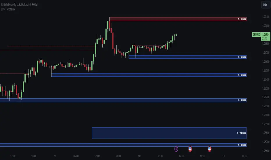
[UST] Protein+Support/Resistance Script: A Comprehensive Overview
Thanks to Pmgjiv for providing the foundation to this improved Version.
In the world of trading, having a robust support and resistance analysis tool can make a significant difference in decision-making and overall strategy. Let's delve into the enhancements made to the support/resistance script and how each component contributes to a trader's arsenal:
Changes and improvements made for the script to help Traders make better rational decisions in their Trading:
1. Multiple Timeframes:
Integrating multiple timeframes into the analysis provides a multi-dimensional view of the market. Traders can now assess price action across different time horizons simultaneously. This feature allows for a deeper understanding of market dynamics and helps in identifying significant support and resistance levels across various timeframes.
2. Timeframe Labels Inside Zones:
By including timeframe labels within the zones, traders can easily identify the origin of each support or resistance level. This contextual information enhances clarity and facilitates more informed decision-making, especially when navigating through multiple timeframes.
3. Visual Zone Update:
Visual updates on zones enable traders to track changes in support and resistance levels in real-time. This dynamic feature enhances the analytical process by providing immediate insights into evolving market conditions, thereby enabling traders to adapt their strategies accordingly.
4. Zones Hit:
Understanding the frequency and intensity of zone hits offers valuable insights into the strength and relevance of support and resistance levels. Traders can gauge the significance of each zone based on its historical interaction with price, thereby gaining a deeper understanding of market sentiment and potential trading opportunities.
5. Option to Turn off Current Timeframe:
The ability to toggle off the current timeframe streamlines chart analysis by focusing only on the most critical support and resistance zones. This decluttering feature helps traders prioritize key levels, reducing cognitive overload and enhancing decision-making efficiency.
Explanation of Additional Functions:
a. Lookback:
The 'lookback' parameter allows traders to customize the age of support and resistance zones based on their trading style and preferences. By adjusting the lookback setting, traders can choose whether to prioritize recent price action or consider historical data, thus tailoring the analysis to their specific trading strategies.
b. Swinglength:
Swinglength determines the sensitivity of the support and resistance zones. By modifying this parameter, traders can control how aggressively the script identifies pivot points. A higher swinglength value results in smoother, more stable zones, whereas a lower value increases sensitivity, capturing smaller price movements.
c. ZigZag Indicator:
The ZigZag indicator plays a pivotal role in identifying significant price reversals. Its period setting determines the number of price bars considered before confirming a pivot point. Traders can utilize this indicator to identify key turning points in the market, aiding in the identification of robust support and resistance levels.
Impact of Sensitivity on Zones:
Adjusting the sensitivity of the ZigZag indicator directly influences the identification and delineation of support and resistance zones. Higher sensitivity levels result in fewer but more robust zones, capturing significant price movements. Conversely, lower sensitivity levels yield more zones, accommodating smaller price fluctuations but potentially introducing noise into the analysis.
d. S/R Range:
The ability to adjust the width of support and resistance zones allows traders to customize the breadth of key areas on a chart. Choosing a wider range encompasses a broader spectrum of prices, thereby identifying more comprehensive support and resistance levels. This flexibility enables traders to adapt their analysis to different market conditions and trading strategies.
Utilization in Trading:
Comprehensive Analysis: By incorporating multiple timeframes, traders gain a holistic view of market dynamics, enabling them to identify high-probability trading opportunities across various horizons.
Contextual Understanding: Timeframe labels within zones provide context, helping traders understand the significance of each level in relation to different timeframes and market conditions.
Real-time Adaptability: Visual zone updates facilitate real-time analysis, allowing traders to adjust their strategies promptly in response to changing market conditions.
Informed Decision-making: By considering zone hits, traders can assess the strength and relevance of support and resistance levels, enhancing their ability to make informed trading decisions.
Customized Analysis: Adjustable parameters such as lookback, swinglength, and sensitivity empower traders to tailor the analysis to their individual trading styles and preferences, enhancing precision and effectiveness.
In summary, these enhancements to the support/resistance script provide traders with a powerful toolkit for analyzing market dynamics, identifying key levels, and executing well-informed trading strategies across various timeframes and market conditions.
Major and Minor Trend Indicator by Nikhil34a V 2.2Title: Major and Minor Trend Indicator by Nikhil34a V 2.2
Description:
The Major and Minor Trend Indicator v2.2 is a comprehensive technical analysis script designed for use with the TradingView platform. This powerful tool is developed in Pine Script version 5 and helps traders identify potential buying and selling opportunities in the stock market.
Features:
SMA Trend Analysis: The script calculates two Simple Moving Averages (SMAs) with user-defined lengths for major and minor trends. It displays these SMAs on the chart, allowing traders to visualize the prevailing trends easily.
Surge Detection: The indicator can detect buying and selling surges based on specific conditions, such as volume, RSI, MACD, and stochastic indicators. Both Buying and Selling surges are marked in black on the chart.
Option Buy Zone Detection: The script identifies the option buy zone based on SMA crossovers, RSI, and MACD values. The buy zone is categorized as "CE Zone" or "PE Zone" and displayed in the table along with the trigger time.
Two-Day High and Low Range: The script calculates the highest high and lowest low of the previous two trading days and plots them on the chart. The area between these points is shaded in semi-transparent green and red colors.
Crossover Analysis: The script analyzes moving average crossovers on multiple timeframes (2-minute, 3-minute, and 5-minute) and displays buy and sell signals accordingly.
Trend Identification: The script identifies the major and minor trends as either bullish or bearish, providing valuable insights into the overall market sentiment.
Usage:
Customize Major and Minor SMA Periods: Adjust the lengths of major and minor SMAs through input parameters to suit your trading preferences.
Enable/Disable Moving Averages: Choose which SMAs to display on the chart by toggling the "showXMA" input options.
Set Surge and Option Buy Zone Thresholds: Modify the surgeThreshold, volumeThreshold, RSIThreshold, and StochThreshold inputs to refine the surge and buy zone detection.
Analyze Crossover Signals: Monitor the crossover signals in the table, categorized by timeframes (2-minute, 3-minute, and 5-minute).
Explore Market Bias and Distance to 2-Day High/Low: The table provides information on market bias, current price movement relative to the previous two-day high and low, and the option buy zone status.
Additional Use Cases:
Surge Indicator:
The script includes a Surge Indicator that detects sudden buying or selling surges in the market. When a buying surge is identified, the "BSurge" label will appear below the corresponding candle with black text on a white background. Similarly, a selling surge will display the "SSurge" label in white text on a black background. These indicators help traders quickly spot strong buying or selling activities that may influence their trading decisions. These surges can be used to identify sudden premium dump zones.
Option Buy Zone:
The Option Buy Zone is an essential feature that identifies potential zones for buying call options (CE Zone) or put options (PE Zone) based on specific technical conditions. The indicator evaluates SMA crossovers, RSI, and MACD values to determine the current market sentiment. When the option buy zone is triggered, the script will display the respective zone ("CE Zone" or "PE Zone") in the table, highlighted with a white background. Additionally, the time when the buy zone was triggered will be shown under the "Option Buy Zone Trigger Time" column.
Price Movement Relative to 2-Day High/Low:
The script calculates the highest high and lowest low of the previous two trading days (high2DaysAgo and low2DaysAgo) and plots these points on the chart. The area between these two points is shaded in semi-transparent green and red colors. The green region indicates the price range between the highpricetoconsider (highest high of the previous two days) and the lower value between highPreviousDay and high2DaysAgo. Similarly, the red region represents the price range between the lowpricetoconsider (lowest low of the previous two days) and the higher value between lowPreviousDay and low2DaysAgo.
Entry Time and Current Zone:
The script identifies potential entry times for trades within the option buy zone. When a valid buy zone trigger occurs, the script calculates the entryTime by adding the durationInMinutes (user-defined) to the startTime. The entryTime will be displayed in the "Entry Time" column of the table. Depending on the comparison between optionbuyzonetriggertime and entryTime, the background color of the entry time will change. If optionbuyzonetriggertime is greater than entryTime, the background color will be yellow, indicating that a new trigger has occurred before the specified duration. Otherwise, the background color will be green, suggesting that the entry time is still within the defined duration.
Current Zone Indicator:
The script further categorizes the current zone as either "CE Zone" (call option zone) or "PE Zone" (put option zone). When the market is trending upwards and the minor SMA is above the major SMA, the currentZone will be set to "CE Zone." Conversely, when the market is trending downwards and the minor SMA is below the major SMA, the currentZone will be "PE Zone." This information is displayed in the "Current Zone" column of the table.
These additional use cases empower traders with valuable insights into market trends, buying and selling surges, option buy zones, and potential entry times. Traders can combine this information with their analysis and risk management strategies to make informed and confident trading decisions.
Note:
The script is optimized for identifying trends and potential trade opportunities. It is crucial to perform additional analysis and risk management before executing any trades based on the provided signals.
Happy Trading!

Possible RSI [Loxx]Possible RSI is a normalized, variety second-pass normalized, Variety RSI with Dynamic Zones and optionl High-Pass IIR digital filtering of source price input. This indicator includes 7 types of RSI.
High-Pass Fitler (optional)
The Ehlers Highpass Filter is a technical analysis tool developed by John F. Ehlers. Based on aerospace analog filters, this filter aims at reducing noise from price data. Ehlers Highpass Filter eliminates wave components with periods longer than a certain value. This reduces lag and makes the oscialltor zero mean. This turns the RSI output into something more similar to Stochasitc RSI where it repsonds to price very quickly.
First Normalization Pass
RSI (Relative Strength Index) is already normalized. Hence, making a normalized RSI seems like a nonsense... if it was not for the "flattening" property of RSI. RSI tends to be flatter and flatter as we increase the calculating period--to the extent that it becomes unusable for levels trading if we increase calculating periods anywhere over the broadly recommended period 8 for RSI. In order to make that (calculating period) have less impact to significant levels usage of RSI trading style in this version a sort of a "raw stochastic" (min/max) normalization is applied.
Second-Pass Variety Normalization Pass
There are three options to choose from:
1. Gaussian (Fisher Transform), this is the default: The Fisher Transform is a function created by John F. Ehlers that converts prices into a Gaussian normal distribution. The normaliztion helps highlights when prices have moved to an extreme, based on recent prices. This may help in spotting turning points in the price of an asset. It also helps show the trend and isolate the price waves within a trend.
2. Softmax: The softmax function, also known as softargmax: or normalized exponential function, converts a vector of K real numbers into a probability distribution of K possible outcomes. It is a generalization of the logistic function to multiple dimensions, and used in multinomial logistic regression. The softmax function is often used as the last activation function of a neural network to normalize the output of a network to a probability distribution over predicted output classes, based on Luce's choice axiom.
3. Regular Normalization (devaitions about the mean): Converts a vector of K real numbers into a probability distribution of K possible outcomes without using log sigmoidal transformation as is done with Softmax. This is basically Softmax without the last step.
Dynamic Zones
As explained in "Stocks & Commodities V15:7 (306-310): Dynamic Zones by Leo Zamansky, Ph .D., and David Stendahl"
Most indicators use a fixed zone for buy and sell signals. Here’ s a concept based on zones that are responsive to past levels of the indicator.
One approach to active investing employs the use of oscillators to exploit tradable market trends. This investing style follows a very simple form of logic: Enter the market only when an oscillator has moved far above or below traditional trading lev- els. However, these oscillator- driven systems lack the ability to evolve with the market because they use fixed buy and sell zones. Traders typically use one set of buy and sell zones for a bull market and substantially different zones for a bear market. And therein lies the problem.
Once traders begin introducing their market opinions into trading equations, by changing the zones, they negate the system’s mechanical nature. The objective is to have a system automatically define its own buy and sell zones and thereby profitably trade in any market — bull or bear. Dynamic zones offer a solution to the problem of fixed buy and sell zones for any oscillator-driven system.
An indicator’s extreme levels can be quantified using statistical methods. These extreme levels are calculated for a certain period and serve as the buy and sell zones for a trading system. The repetition of this statistical process for every value of the indicator creates values that become the dynamic zones. The zones are calculated in such a way that the probability of the indicator value rising above, or falling below, the dynamic zones is equal to a given probability input set by the trader.
To better understand dynamic zones, let's first describe them mathematically and then explain their use. The dynamic zones definition:
Find V such that:
For dynamic zone buy: P{X <= V}=P1
For dynamic zone sell: P{X >= V}=P2
where P1 and P2 are the probabilities set by the trader, X is the value of the indicator for the selected period and V represents the value of the dynamic zone.
The probability input P1 and P2 can be adjusted by the trader to encompass as much or as little data as the trader would like. The smaller the probability, the fewer data values above and below the dynamic zones. This translates into a wider range between the buy and sell zones. If a 10% probability is used for P1 and P2, only those data values that make up the top 10% and bottom 10% for an indicator are used in the construction of the zones. Of the values, 80% will fall between the two extreme levels. Because dynamic zone levels are penetrated so infrequently, when this happens, traders know that the market has truly moved into overbought or oversold territory.
Calculating the Dynamic Zones
The algorithm for the dynamic zones is a series of steps. First, decide the value of the lookback period t. Next, decide the value of the probability Pbuy for buy zone and value of the probability Psell for the sell zone.
For i=1, to the last lookback period, build the distribution f(x) of the price during the lookback period i. Then find the value Vi1 such that the probability of the price less than or equal to Vi1 during the lookback period i is equal to Pbuy. Find the value Vi2 such that the probability of the price greater or equal to Vi2 during the lookback period i is equal to Psell. The sequence of Vi1 for all periods gives the buy zone. The sequence of Vi2 for all periods gives the sell zone.
In the algorithm description, we have: Build the distribution f(x) of the price during the lookback period i. The distribution here is empirical namely, how many times a given value of x appeared during the lookback period. The problem is to find such x that the probability of a price being greater or equal to x will be equal to a probability selected by the user. Probability is the area under the distribution curve. The task is to find such value of x that the area under the distribution curve to the right of x will be equal to the probability selected by the user. That x is the dynamic zone.
7 Types of RSI
See here to understand which RSI types are included:
Included:
Bar coloring
4 signal types
Alerts
Loxx's Expanded Source Types
Loxx's Variety RSI
Loxx's Dynamic Zones

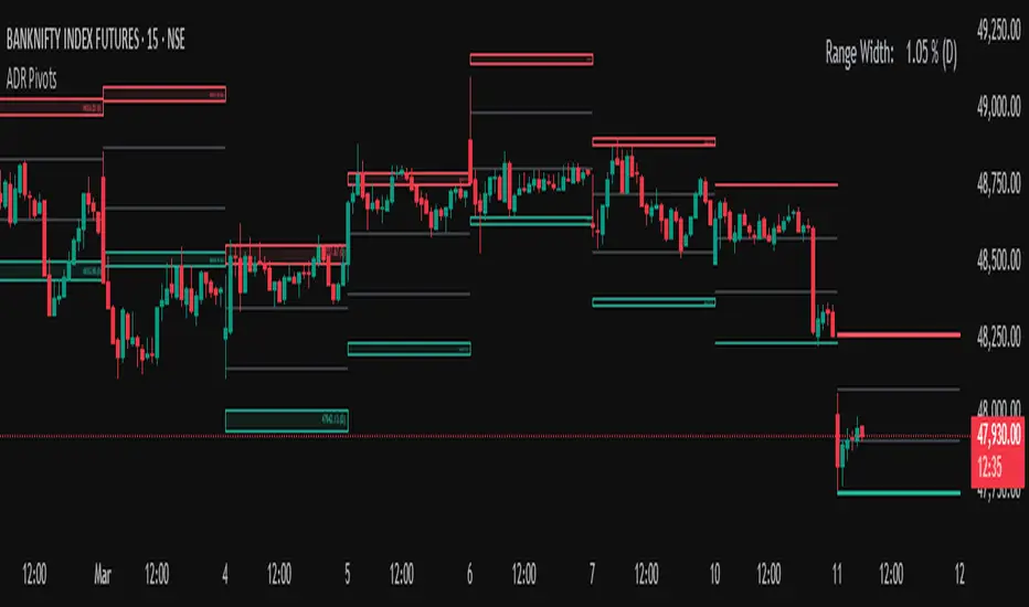
Average Daily Range (ADR) (Multi Timeframe, Multi Period)Average Daily Range (ADR)
(Multi Timeframe, Multi Period, Extended Levels)
Tips
• Narrow Zones are an indication of breakouts. It can be a very tight range as well.
• Wider Zones can be Sideways or Volatile.
What is this Indicator?
• This is Average Daily Range (ADR) Zones or Pivots.
• This have Multi Timeframe, Multi Period (Up to 3 Levels) and Extended Target Levels.
Advantages of this Indicator
• This is a Leading indicator, not Dynamic or Repaint.
• Helps to identify the reversal points.
• The levels are more accurate and not like the old formulas.
• Can practically follow the Buy Low and Sell High principle.
• Helps to keep minimum Stop Loss.
Who to use?
• Highly beneficial for Day Traders
• It can be used for Swing and Positions as well.
What timeframe to use?
• Any timeframe.
When to use?
• Any market conditions.
How to use?
Entry
• Long entry when the Price reach at or closer to the Green Support zone.
• Long entry when the Price retrace to the Red Resistance zone.
• Short entry when the Price reach at or closer to the Red Resistance zone.
• Short entry when the Price retrace to the Green Support zone.
• Long or Short at the Pivot line.
Exit
• Use past ADR levels as targets.
• Or use the Target levels in the indicator for breakouts.
• Use the Pivot line as target.
• Use Support or Resistance Zones as targets in reversal method.
What are the Lines?
Gray Line:
• It the day Open or can be considered as Pivot.
Red & Green ADR Zones:
• Red Zone is Resistance.
• Green Zone is Support.
• Mostly price can reverse from this Zones.
• Multiple Red and Green Lines forms a Zone.
• These lines are average levels of past days which helps to figure out the maximum and minimum price range that can be moved in that day.
• The default number of days are 5, 7 and 14. This can be customized.
Red & Green Target Lines:
• These are Target levels.
What are the Labels?
• First Number: Price of that level.
• Numbers in (): Percentage change and Change of price from LTP (Last Traded Price) to that Level.
General Tips
• It is good if Stock trend is same as that of the Index trend.
• Lots of indicators creates lots of confusion.
• Keep the chart simple and clean.
• Buy Low and Sell High.
• Master averages or 50%.
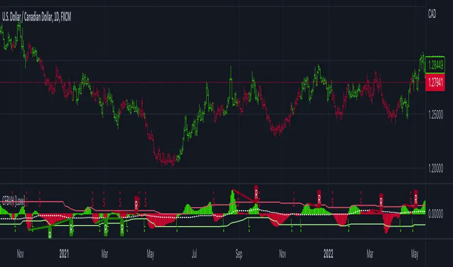
CFB-Adaptive Velocity Histogram [Loxx]CFB-Adaptive Velocity Histogram is a velocity indicator with One-More-Moving-Average Adaptive Smoothing of input source value and Jurik's Composite-Fractal-Behavior-Adaptive Price-Trend-Period input with Dynamic Zones. All Juirk smoothing allows for both single and double Jurik smoothing passes. Velocity is adjusted to pips but there is no input value for the user. This indicator is tuned for Forex but can be used on any time series data.
What is Composite Fractal Behavior ( CFB )?
All around you mechanisms adjust themselves to their environment. From simple thermostats that react to air temperature to computer chips in modern cars that respond to changes in engine temperature, r.p.m.'s, torque, and throttle position. It was only a matter of time before fast desktop computers applied the mathematics of self-adjustment to systems that trade the financial markets.
Unlike basic systems with fixed formulas, an adaptive system adjusts its own equations. For example, start with a basic channel breakout system that uses the highest closing price of the last N bars as a threshold for detecting breakouts on the up side. An adaptive and improved version of this system would adjust N according to market conditions, such as momentum, price volatility or acceleration.
Since many systems are based directly or indirectly on cycles, another useful measure of market condition is the periodic length of a price chart's dominant cycle, (DC), that cycle with the greatest influence on price action.
The utility of this new DC measure was noted by author Murray Ruggiero in the January '96 issue of Futures Magazine. In it. Mr. Ruggiero used it to adaptive adjust the value of N in a channel breakout system. He then simulated trading 15 years of D-Mark futures in order to compare its performance to a similar system that had a fixed optimal value of N. The adaptive version produced 20% more profit!
This DC index utilized the popular MESA algorithm (a formulation by John Ehlers adapted from Burg's maximum entropy algorithm, MEM). Unfortunately, the DC approach is problematic when the market has no real dominant cycle momentum, because the mathematics will produce a value whether or not one actually exists! Therefore, we developed a proprietary indicator that does not presuppose the presence of market cycles. It's called CFB (Composite Fractal Behavior) and it works well whether or not the market is cyclic.
CFB examines price action for a particular fractal pattern, categorizes them by size, and then outputs a composite fractal size index. This index is smooth, timely and accurate
Essentially, CFB reveals the length of the market's trending action time frame. Long trending activity produces a large CFB index and short choppy action produces a small index value. Investors have found many applications for CFB which involve scaling other existing technical indicators adaptively, on a bar-to-bar basis.
What is Jurik Volty used in the Juirk Filter?
One of the lesser known qualities of Juirk smoothing is that the Jurik smoothing process is adaptive. "Jurik Volty" (a sort of market volatility ) is what makes Jurik smoothing adaptive. The Jurik Volty calculation can be used as both a standalone indicator and to smooth other indicators that you wish to make adaptive.
What is the Jurik Moving Average?
Have you noticed how moving averages add some lag (delay) to your signals? ... especially when price gaps up or down in a big move, and you are waiting for your moving average to catch up? Wait no more! JMA eliminates this problem forever and gives you the best of both worlds: low lag and smooth lines.
Ideally, you would like a filtered signal to be both smooth and lag-free. Lag causes delays in your trades, and increasing lag in your indicators typically result in lower profits. In other words, late comers get what's left on the table after the feast has already begun.
What are Dynamic Zones?
As explained in "Stocks & Commodities V15:7 (306-310): Dynamic Zones by Leo Zamansky, Ph .D., and David Stendahl"
Most indicators use a fixed zone for buy and sell signals. Here’ s a concept based on zones that are responsive to past levels of the indicator.
One approach to active investing employs the use of oscillators to exploit tradable market trends. This investing style follows a very simple form of logic: Enter the market only when an oscillator has moved far above or below traditional trading lev- els. However, these oscillator- driven systems lack the ability to evolve with the market because they use fixed buy and sell zones. Traders typically use one set of buy and sell zones for a bull market and substantially different zones for a bear market. And therein lies the problem.
Once traders begin introducing their market opinions into trading equations, by changing the zones, they negate the system’s mechanical nature. The objective is to have a system automatically define its own buy and sell zones and thereby profitably trade in any market — bull or bear. Dynamic zones offer a solution to the problem of fixed buy and sell zones for any oscillator-driven system.
An indicator’s extreme levels can be quantified using statistical methods. These extreme levels are calculated for a certain period and serve as the buy and sell zones for a trading system. The repetition of this statistical process for every value of the indicator creates values that become the dynamic zones. The zones are calculated in such a way that the probability of the indicator value rising above, or falling below, the dynamic zones is equal to a given probability input set by the trader.
To better understand dynamic zones, let's first describe them mathematically and then explain their use. The dynamic zones definition:
Find V such that:
For dynamic zone buy: P{X <= V}=P1
For dynamic zone sell: P{X >= V}=P2
where P1 and P2 are the probabilities set by the trader, X is the value of the indicator for the selected period and V represents the value of the dynamic zone.
The probability input P1 and P2 can be adjusted by the trader to encompass as much or as little data as the trader would like. The smaller the probability, the fewer data values above and below the dynamic zones. This translates into a wider range between the buy and sell zones. If a 10% probability is used for P1 and P2, only those data values that make up the top 10% and bottom 10% for an indicator are used in the construction of the zones. Of the values, 80% will fall between the two extreme levels. Because dynamic zone levels are penetrated so infrequently, when this happens, traders know that the market has truly moved into overbought or oversold territory.
Calculating the Dynamic Zones
The algorithm for the dynamic zones is a series of steps. First, decide the value of the lookback period t. Next, decide the value of the probability Pbuy for buy zone and value of the probability Psell for the sell zone.
For i=1, to the last lookback period, build the distribution f(x) of the price during the lookback period i. Then find the value Vi1 such that the probability of the price less than or equal to Vi1 during the lookback period i is equal to Pbuy. Find the value Vi2 such that the probability of the price greater or equal to Vi2 during the lookback period i is equal to Psell. The sequence of Vi1 for all periods gives the buy zone. The sequence of Vi2 for all periods gives the sell zone.
In the algorithm description, we have: Build the distribution f(x) of the price during the lookback period i. The distribution here is empirical namely, how many times a given value of x appeared during the lookback period. The problem is to find such x that the probability of a price being greater or equal to x will be equal to a probability selected by the user. Probability is the area under the distribution curve. The task is to find such value of x that the area under the distribution curve to the right of x will be equal to the probability selected by the user. That x is the dynamic zone.
Included:
Bar coloring
3 signal variations w/ alerts
Divergences w/ alerts
Loxx's Expanded Source Types
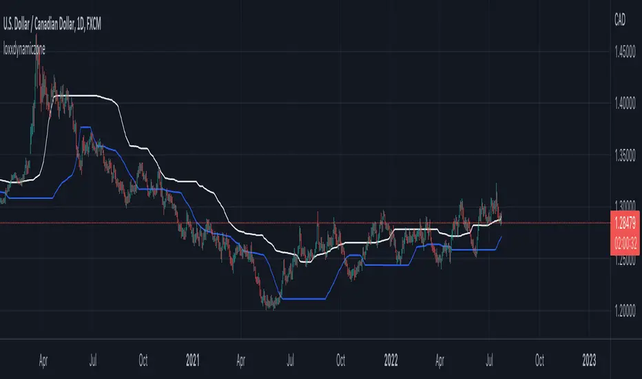
loxxdynamiczoneLibrary "loxxdynamiczone"
Dynamic Zones
Derives Leo Zamansky and David Stendahl's Dynamic Zone,
see "Stocks & Commodities V15:7 (306-310): Dynamic Zones by Leo Zamansky, Ph .D., and David Stendahl"
What are Dynamic Zones?
As explained in "Stocks & Commodities V15:7 (306-310): Dynamic Zones by Leo Zamansky, Ph .D., and David Stendahl"
Most indicators use a fixed zone for buy and sell signals. Here’ s a concept based on zones that are responsive to past levels of the indicator.
One approach to active investing employs the use of oscillators to exploit tradable market trends. This investing style follows a very simple form of logic: Enter the market only when an oscillator has moved far above or below traditional trading lev- els. However, these oscillator- driven systems lack the ability to evolve with the market because they use fixed buy and sell zones. Traders typically use one set of buy and sell zones for a bull market and substantially different zones for a bear market. And therein lies the problem.
Once traders begin introducing their market opinions into trading equations, by changing the zones, they negate the system’s mechanical nature. The objective is to have a system automatically define its own buy and sell zones and thereby profitably trade in any market — bull or bear. Dynamic zones offer a solution to the problem of fixed buy and sell zones for any oscillator-driven system.
An indicator’s extreme levels can be quantified using statistical methods. These extreme levels are calculated for a certain period and serve as the buy and sell zones for a trading system. The repetition of this statistical process for every value of the indicator creates values that become the dynamic zones. The zones are calculated in such a way that the probability of the indicator value rising above, or falling below, the dynamic zones is equal to a given probability input set by the trader.
To better understand dynamic zones, let's first describe them mathematically and then explain their use. The dynamic zones definition:
Find V such that:
For dynamic zone buy: P{X <= V}=P1
For dynamic zone sell: P{X >= V}=P2
where P1 and P2 are the probabilities set by the trader, X is the value of the indicator for the selected period and V represents the value of the dynamic zone.
The probability input P1 and P2 can be adjusted by the trader to encompass as much or as little data as the trader would like. The smaller the probability, the fewer data values above and below the dynamic zones. This translates into a wider range between the buy and sell zones. If a 10% probability is used for P1 and P2, only those data values that make up the top 10% and bottom 10% for an indicator are used in the construction of the zones. Of the values, 80% will fall between the two extreme levels. Because dynamic zone levels are penetrated so infrequently, when this happens, traders know that the market has truly moved into overbought or oversold territory.
Calculating the Dynamic Zones
The algorithm for the dynamic zones is a series of steps. First, decide the value of the lookback period t. Next, decide the value of the probability Pbuy for buy zone and value of the probability Psell for the sell zone.
For i=1, to the last lookback period, build the distribution f(x) of the price during the lookback period i. Then find the value Vi1 such that the probability of the price less than or equal to Vi1 during the lookback period i is equal to Pbuy. Find the value Vi2 such that the probability of the price greater or equal to Vi2 during the lookback period i is equal to Psell. The sequence of Vi1 for all periods gives the buy zone. The sequence of Vi2 for all periods gives the sell zone.
In the algorithm description, we have: Build the distribution f(x) of the price during the lookback period i. The distribution here is empirical namely, how many times a given value of x appeared during the lookback period. The problem is to find such x that the probability of a price being greater or equal to x will be equal to a probability selected by the user. Probability is the area under the distribution curve. The task is to find such value of x that the area under the distribution curve to the right of x will be equal to the probability selected by the user. That x is the dynamic zone.
dZone(type, src, pval, per)
method for retrieving the dynamic zone levels from input source.
Parameters:
type : string, value of either 'buy' or 'sell'.
src : float, source, either regular source type or some other caculated value.
pval : float, probability defined by extension over/under source, a number <= 1.0.
per : int, period lookback.
Returns: float dynamic zone level.
usage:
dZone("buy", close, 0.2, 70)
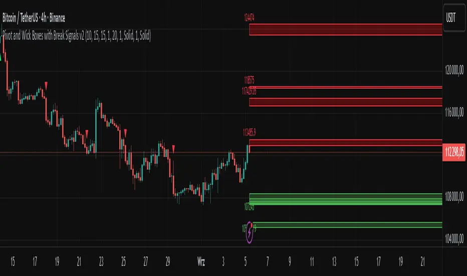
Pivot and Wick Boxes with Break Signals v2█ OVERVIEW
The "Pivot and Wick Boxes with Break Signals v2" is an advanced Pine Script® technical analysis tool that identifies pivot points (highs and lows) on the chart and draws customizable boxes based on the wicks of pivot candles. It is ideal for traders using price action strategies, helping to identify key support and resistance levels and potential breakout trading opportunities. With flexible settings, a volume filter, and label grouping, the indicator ensures clarity and precision on the chart.
█ CONCEPTS
The indicator modifies how zones are drawn, displaying boxes on the latest candle rather than extending from the zones based on pivot candle wicks. This approach prevents visual clutter on the chart, allowing simultaneous use of other indicators without sacrificing clarity.
Why are wicks important?Wicks of pivot candles indicate significant market reactions in key areas. Depending on the context, they may signal rejection, testing, or absorption of support or resistance levels. Long wicks often appear where large players are active, and the marked zones are frequently retested. The indicator enables quick identification and observation of their impact on future price movements.
█ FEATURES
Pivot Detection: Identifies pivot points (highs and lows) based on a user-defined lookback period (Pivot Length), with options to display boxes for high and low pivot candle wicks separately.
Customizable Boxes: Draws boxes based on pivot candle wicks with adjustable border colors, background gradients, border styles (solid, dashed, dotted), and border widths.
Breakout Signals: Generates buy (green upward triangle) and sell (red downward triangle) signals when the price breaks through a pivot and the candle closes on the opposite side, indicating potential trend continuation. If the price approaches a pivot zone but fails to break it, this may suggest a potential trend reversal or the end of a correction.
Volume Filter: Optional volume-based signal filter that requires breakouts to have a volume exceeding a user-defined multiplier of the average volume over a specified period. Note: the volume filter will not work on markets where volume data is unavailable.
Label Grouping: Automatically groups overlapping pivot labels to avoid chart clutter, displaying only key price levels.
█ HOW TO USE
Add to Chart: Apply the indicator to your TradingView chart via the Pine Editor or Indicators menu.
Configure Settings:
Pivot Settings: Adjust Pivot Length to change the sensitivity of pivot detection—the value represents the number of candles, which equals the delay in displaying the pivot. Larger values generate fewer pivots, but they are generally more significant. Set Max High Pivot Boxes and Max Low Pivot Boxes to control the number of displayed boxes.
Signal Settings: Enable Use Volume Filter for Signals to require higher volume for breakouts, and adjust Average Volume Multiplier and Average Volume Period. A volume multiplier of 1 means the filter allows pivots with a volume equal to or greater than the average volume over the specified period.
Box Styling: Configure border colors, background gradients, line thickness, and border styles for high and low pivot boxes.
Interpreting Signals:
Buy Signal: A green triangle below the bar indicates a breakout above a high pivot box, suggesting potential continuation of an uptrend.
Sell Signal: A red triangle above the bar indicates a breakout below a low pivot box, suggesting potential continuation of a downtrend.
Non-Breakout Zones: If the price approaches a pivot zone but fails to break it, it may indicate a potential trend reversal or the end of a correction (e.g., price rejection at a resistance level in a downtrend or a support level in an uptrend).
Overlapping Zones: If pivot zones overlap, it indicates the level has been tested multiple times, suggesting its significance in the market.
Use signals in conjunction with other technical analysis tools for confirmation.
Monitoring Levels: Use labeled pivot levels as potential support and resistance zones for trade planning.
█ APPLICATIONS
Price Action Trading: Use pivot levels as support and resistance zones. For example, in an uptrend, you can look for buying opportunities near low pivot zones (support), where price often bounces after testing the wick of a pivot candle. Combining with other indicators, such as Fibonacci levels, enhances the significance of pivot zones—if they align with Fibonacci levels and are accompanied by high volume, the zone is considered stronger.
Breakout Strategies: Trade based on breakout signals from key pivot zones. A buy signal after a breakout from a high pivot with confirmed volume may indicate continued upward movement. Using the indicator with other tools, such as moving averages or RSI, can help confirm the strength of the breakout.
Practical Approach:
The more frequently a zone is tested in a short period, the higher the risk of a breakout, as supply or demand may be exhausted.
The longer a zone holds without breaking, the more significant it becomes for the market, both psychologically and technically.
As the saying goes: “A zone is strong until it breaks—when it does, a strong move often follows.”
How to observe?
Strong bounces from a zone indicate that demand or supply remains active.
Weaker bounces or price lingering near the level may suggest the market is preparing for a breakout.
█ NOTES
Test the indicator across different timeframes and markets (stocks, forex, crypto) to optimize settings for your trading style.
The volume filter will not work on markets where volume data is unavailable. In such cases, disable the volume filter in the settings.
For best results, use on high-liquidity markets when the volume filter is enabled.
Dynamic Liquidity Depth [BigBeluga]
Dynamic Liquidity Depth
A liquidity mapping engine that reveals hidden zones of market vulnerability. This tool simulates where potential large concentrations of stop-losses may exist — above recent highs (sell-side) and below recent lows (buy-side) — by analyzing real price behavior and directional volume. The result is a dynamic two-sided volume profile that highlights where price is most likely to gravitate during liquidation events, reversals, or engineered stop hunts.
🔵 KEY FEATURES
Two-Sided Liquidity Profiles:
Plots two separate profiles on the chart — one above price for potential sell-side liquidity , and one below price for potential buy-side liquidity . Each profile reflects the volume distribution across binned zones derived from historical highs and lows.
Real Stop Zone Simulation:
Each profile is offset from the current high or low using an ATR-based buffer. This simulates where traders might cluster their stop-losses above swing highs (short stops) or below swing lows (long stops).
Directional Volume Analysis:
Buy-side volume is accumulated only from bullish candles (close > open), while sell-side volume is accumulated only from bearish candles (close < open). This directional filtering enhances accuracy by capturing genuine pressure zones.
Dynamic Volume Heatmap:
Each liquidity bin is rendered as a horizontal box with a color gradient based on volume intensity:
- Low activity bins are shaded lightly.
- High-volume zones appear more vividly in red (sell) or lime (buy).
- The maximum volume bin in each profile is emphasized with a brighter fill and a volume label.
Extended POC Zones:
The Point of Control (PoC) — the bin with the most volume — is extended backwards across the entire lookback period to mark critical resistance (sell-side) or support (buy-side) levels.
Total Volume Summary Labels:
At the center of each profile, a summary label displays Total Buy Liquidity and Total Sell Liquidity volume.
This metric helps assess directional imbalance — when buy liquidity is dominant, the market may favor upward continuation, and vice versa.
Customizable Profile Granularity:
You can fine-tune both Resolution (Bins) and Offset Distance to adjust how far profiles are displaced from price and how many levels are calculated within the ATR range.
🔵 HOW IT WORKS
The indicator calculates an ATR-based buffer above highs and below lows to define the top and bottom of the liquidity zones.
Using a user-defined lookback period, it scans historical candles and divides the buffered zones into bins.
Each bin checks if bullish (or bearish) candles pass through it based on price wicks and body.
Volume from valid candles is summed into the corresponding bin.
When volume exists in a bin, a horizontal box is drawn with a width scaled by relative volume strength.
The bin with the highest volume is highlighted and optionally extended backward as a zone of importance.
Total buy/sell liquidity is displayed with a summary label at the side of the profile.
🔵 USAGE/b]
Identify Stop Hunt Zones: High-volume clusters near swing highs/lows are likely liquidation zones targeted during fakeouts.
Fade or Follow Reactions: Price hitting a high-volume bin may reverse (fade opportunity) or break with strength (confirmation breakout).
Layer with Other Tools: Combine with market structure, order blocks, or trend filters to validate entries near liquidity.
Adjust Offset for Sensitivity: Use higher offset to simulate wider stop placement; use lower for tighter scalping zones.
🔵 CONCLUSION
Dynamic Liquidity Depth transforms raw price and volume into a spatial map of liquidity. By revealing areas where stop orders are likely hidden, it gives traders insight into price manipulation zones, potential reversal levels, and breakout traps. Whether you're hunting for traps or trading with the flow, this tool equips you to navigate liquidity with precision.

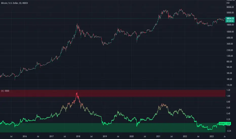
Bitcoin Economics Adaptive MultipleBEAM (Bitcoin Economics Adaptive Multiple) is an indicator that assesses the valuation of Bitcoin by dividing the current price of Bitcoin by a moving average of past prices. Its purpose is to provide insights into whether Bitcoin is under or overvalued at any given time. The thresholds for the buy and sell zones in BEAM are adjustable, allowing users to customize the indicator based on their preferences and trading strategies.
BEAM categorizes Bitcoin's valuation into two distinct zones: the green buy zone and the red sell zone.
Green Buy Zone:
The green buy zone in BEAM indicates that Bitcoin is potentially undervalued. Traders and investors may interpret this zone as a favorable buying opportunity. The threshold for the buy zone can be adjusted to suit individual preferences or trading strategies.
Red Sell Zone:
The red sell zone in BEAM suggests that Bitcoin is potentially overvalued. Traders and investors may consider selling their Bitcoin holdings during this zone to secure profits or manage risk. The threshold for the sell zone is adjustable, allowing users to adapt the indicator based on their trading preferences.
Methodology:
BEAM calculates the indicator value using the following formula:
beam = math.log(close / ta.sma(close, math.min(count, 1400))) / 2.5
The calculation involves taking the natural logarithm of the ratio between the current price of Bitcoin and a simple moving average of past prices. The moving average period used is a minimum of the specified count or 1400, providing a suitable historical reference for valuation assessment.
The resulting value of BEAM provides a standardized measure that can be compared across different time periods. By adjusting the thresholds for the buy and sell zones, users can customize BEAM to their preferred levels of undervaluation and overvaluation.
Utility:
BEAM serves as a tool for investors in the Bitcoin market, offering insights into Bitcoin's valuation and potential buying or selling opportunities. By monitoring BEAM, market participants can gauge whether Bitcoin is potentially undervalued or overvalued, helping them make informed decisions regarding their Bitcoin positions.
It is important to note that BEAM should be used in conjunction with other technical and fundamental analysis tools to validate signals and avoid relying solely on this indicator for trading decisions. Additionally, traders and investors are encouraged to adjust the threshold values based on their specific trading strategies, risk tolerance, and market conditions.
Credit: The BEAM (Bitcoin Economics Adaptive Multiple) indicator was originally developed by BitcoinEcon
Buyside & Sellside Liquidity [LuxAlgo]The Buyside & Sellside Liquidity indicator aims to detect & highlight the first and arguably most important concept within the ICT trading methodology, Liquidity levels.
🔶 SETTINGS
🔹 Liquidity Levels
Detection Length: Lookback period
Margin: Sets margin/sensitivity for a liquidity level detection
🔹 Liquidity Zones
Buyside Liquidity Zones: Enables display of the buyside liquidity zones.
Margin: Sets margin/sensitivity for the liquidity zone boundaries.
Color: Color option for buyside liquidity levels & zones.
Sellside Liquidity Zones: Enables display of the sellside liquidity zones.
Margin: Sets margin/sensitivity for the liquidity zone boundaries.
Color: Color option for sellside liquidity levels & zones.
🔹 Liquidity Voids
Liquidity Voids: Enables display of both bullish and bearish liquidity voids.
Label: Enables display of a label indicating liquidity voids.
🔹 Display Options
Mode: Controls the lookback length of detection and visualization, where Present assumes last 500 bars and Historical assumes all data available to the user
# Visible Levels: Controls the amount of the liquidity levels/zones to be visualized.
🔶 USAGE
Definitions of Liquidity refer to the availability of orders at specific price levels in the market, allowing transactions to occur smoothly.
In the context of Inner Circle Trader's teachings, liquidity mainly relates to stop losses or pending orders and liquidity level/pool, highlighting a concentration of buy or sell orders at specific price levels. Smart money traders, such as banks and other large institutions, often target these liquidity levels/pools to accumulate or distribute their positions.
There are two types of liquidity; Buyside liquidity and Sellside liquidity .
Buyside liquidity represents a level on the chart where short sellers will have their stops positioned, and Sellside liquidity represents a level on the chart where long-biased traders will place their stops.
These areas often act as support or resistance levels and can provide trading opportunities.
When the liquidity levels are breached at which many stop/limit orders are placed have been traded through, the script will create a zone aiming to provide additional insight to figure out the odds of the next price action.
Reversal: It’s common that the price may reverse course and head in the opposite direction, seeking liquidity at the opposite extreme.
Continuation: When the zone is also broken it is a sign for continuation price action.
It's worth noting that ICT concepts are specific to the methodology developed by Michael J. Huddleston and may not align with other trading approaches or strategies.
🔶 DETAILS
Liquidity voids are sudden changes in price when the price jumps from one level to another. Liquidity voids will appear as a single or a group of candles that are all positioned in the same direction. These candles typically have large real bodies and very short wicks, suggesting very little disagreement between buyers and sellers. The peculiar thing about liquidity voids is that they almost always fill up.
🔶 ALERTS
When an alert is configured, the user will have the ability to be notified in case;
Liquidity level is detected/updated.
Liquidity level is breached.
🔶 RELATED SCRIPTS
ICT-Concepts
ICT-Macros
Imbalance-Detector

Dow Theory Cockpit1. Evolution History
The system has reached its final form through five distinct development phases:
Phase 1: Logic Development (V1–V6)
Established four core logics: BREAK and DIP (Dow Theory), SNIPER (Reversal), and PUSH (Trend continuation).
Implemented the Multi-Timeframe (MTF) panel and Market Scanner.
Phase 2: Strategy Transition (V7–V9)
Integrated backtesting features, but found the Pine Script calculation load too heavy for real-time charting.
Phase 3: Optimization & Performance (V10–V11)
Prioritized smooth real-time execution by returning to a lightweight indicator format.
Introduced the on-chart stats panel for Win Rate and P&L tracking.
Phase 4: Visual Completion (V12–V13)
High-Vis Fib: Bold orange lines highlighting the Golden Zone (38.2%/61.8%).
Visual Zones: Introduced Green and Red bands for intuitive trade tracking.
Phase 5: Smart Adjust Implementation (V14 - Current)
Barrier Avoidance: Automatically detects nearby Support/Resistance boxes and shortens the TP to secure profits before a potential reversal.
Dynamic RR Optimization: Automatically adjusts the SL in tandem with the shortened TP to maintain a healthy Risk-Reward ratio.
2. Specifications
Name: Dow Theory Cockpit
Format: Indicator
Trading Style: Scalping to Day Trading
Timeframes: 5M, 15M (Recommended), 1H
Assets: All pairs (Gold, Crypto, Forex, Indices)
3. Features
① Quad-Logic Entry Signals
🎯 SNIPER: Reversal logic targeting "Tops and Bottoms" when the market is overextended.
🌊 DIP: Trend-following logic for "Deep Pullbacks" with clean Moving Average alignment.
⚡ PUSH: Scalping logic for "Shallow Pullbacks" during high-momentum trends.
🚀 BREAK: Classic Dow Theory momentum entry on recent High/Low breakouts.
② Visual Analysis Tools
S/R BOX: Displays key price levels as shaded zones to account for market noise and wick volatility.
High-Vis Auto Fib: Automatically plots Fibonacci levels, highlighting the Golden Zone with bold lines.
③ Bulletproof Money Management
Calculated Lot Size: Displays the precise lot size based on your account balance and Risk % directly on the signal label.
TP/SL Zones: Dynamic Green and Red bands show exactly where your profit and loss targets lie.
④ Smart Adjust Function (NEW)
Logic: Automatically scans for strong S/R walls near your entry.
Normal Condition: Displays TP/SL at your default Risk-Reward ratio.
Wall Detected: Automatically pulls the TP to the edge of the barrier and tightens the SL to maintain the ratio.
Alert: A "⚠️Adj" warning appears on the label when this adjustment is active.
⑤ Integrated Info Panel
Main Panel: Trends across all timeframes, real-time Win Rate, and Period Net P&L.
Scanner: Constant monitoring of Gold/JPY/BTC and major US/JP economic data.
4. How to Use
Configuration: In the settings under , input your balance and Risk %. Set your start date in .
Entry Decision: Wait for the "★ BUY" or "★ SELL" label.
"⚠️Adj" displayed: The system has detected a nearby barrier and narrowed the TP/SL for safety. This results in a higher win rate with smaller gains.
No warning: No barriers detected. Targets the default wide Risk-Reward ratio.
Execution: Enter using the exact Lot size on the label. Set your Limit/Stop orders at the provided TP/SL prices.
Exit: The trade concludes when the price reaches the Green or Red zone. Smart Adjust ensures you exit the market before a potential bounce.
1. 大幅なアップデート履歴 (Evolution History)
このシステムは、以下の5つのフェーズを経て完成しました。
フェーズ1:ロジック構築期 (V1〜V6)
ダウ理論に基づく「BREAK」「DIP」に加え、逆張り「SNIPER」、順張り追撃「PUSH」の4つのロジックを搭載。
マルチタイムフレーム(MTF)パネル、市場監視スキャナーの実装。
フェーズ2:ストラテジー化への挑戦 (V7〜V9)
バックテスト機能を搭載したが、Pine Scriptの計算負荷増大によりチャート動作が重くなる問題が発生。
フェーズ3:軽量化と原点回帰 (V10〜V11)
**「実戦での快適さ」**を最優先し、indicator 形式へ戻して超軽量化。
期間損益や勝率を、チャート上のパネルで簡易確認できる仕様に変更。
フェーズ4:視認性の完成 (V12〜V13)
High-Vis Fib: フィボナッチの重要ライン(38.2%/61.8%)を太いオレンジ実線で強調。
Visual Zone: トレード中、チャート上に「緑(利益)/赤(損失)」の帯を表示し、直感的な判断を可能に。
フェーズ5:スマート・アジャスト実装 (V14 - Current)
障害物回避機能: エントリー方向の直近に「逆側のレジサポBOX(壁)」がある場合、TPをその手前に自動短縮し、反発による含み益消滅リスクを回避。
RR自動最適化: TPの短縮に合わせて、最低限のリスクリワード(RR)を維持するようSLも自動調整する機能を搭載。
2. 全体の仕様 (Specifications)
名称: Dow Theory Cockpit
形式: インジケーター (Indicator)
※TradingViewの「ストラテジーテスター」タブは使用しません。
推奨スタイル: スキャルピング 〜 デイトレード
推奨時間足: 5分足、15分足(推奨)、1時間足
通貨ペア: 全通貨対応(Gold, Crypto, Forex, Index)
3. 特徴と機能 (Features)
① 4つの「高期待値」エントリーロジック
相場の状況に合わせて最適なサインが点灯します。
🎯 SNIPER: 行き過ぎた相場の反転(天底)を狙う逆張り。
🌊 DIP: 移動平均線の並びが良い状態での「深い押し目」を拾う順張り。
⚡ PUSH: 強いトレンド(ADX上昇中)の「浅い押し目」で飛び乗るスキャルピング用。
🚀 BREAK: ダウ理論の基本、直近高値・安値ブレイクでのエントリー。
② 視覚的環境認識ツール
レジサポ BOX: 重要価格帯を「面(ボックス)」で表示。ヒゲのダマシを許容します。
High-Vis Auto Fib: 直近の波を検知し、38.2%/61.8%(ゴールデンゾーン)を太線で強調表示。
③ 鉄壁の資金管理 (Money Management)
推奨ロット表示: 口座資金と許容リスク(%)に基づき、適正ロット数を自動計算して表示します。
TP/SL ゾーン: エントリー中、チャート上に「利確までの緑の帯」と「損切までの赤の帯」が表示され、価格の進行度合いが一目で分かります。
④ スマート・アジャスト機能 (Smart Adjust) ★NEW
機能: エントリー時、目標地点の手前に「強力なレジサポBOX」があるかを自動検知します。
動作:
通常時: 設定通りのRR(2.5倍など)でTP/SLを表示。
壁がある時: **「壁の手前」**にTPを引き下げ、それに合わせてSLも浅く調整します。
表示: 調整が行われた場合、ラベルに 「⚠️Adj(調整済み)」 と警告が出ます。
⑤ 情報集約パネル
Main Panel: 全時間足のトレンド方向、直近の勝率、期間内の純損益を表示。
Scanner: Gold / JPY / BTC の動向と、日米経済指標を常時監視。
4. 使い方 (How to Use)
STEP 1: 初期設定
インジケーター設定の 【F. 資金管理】 を開き、口座資金 と リスク(%) を入力します。
【T. バックテスト期間】 で損益計算を開始したい日付を設定します。
STEP 2: エントリー判断
チャートに 「★ BUY」 または 「★ SELL」 のラベルが出現するのを待ちます。
ラベルの確認:
「⚠️Adj」 と出ている場合 → 「近くに壁があるため、TP/SLを狭く調整しました」という意味です。勝率は上がりますが、値幅は小さくなります。
何も出ていない場合 → 「障害物なし。通常のRRで大きく狙います」という意味です。
STEP 3: 注文 (Execution)
ラベルの数値を信頼して注文を出します。
Lot: 表示された数量を入力。
TP/SL: 表示された価格に指値・逆指値を置く。
STEP 4: 決済 (Exit)
チャート上の 「緑の帯(TP)」 か 「赤の帯(SL)」 にローソク足が到達したら決済です。
**「スマートアジャスト」により、壁の手前で利確設定されているため、「反発して戻ってくる前に逃げ切る」**ことができます。

Dow Theory Cockpit [Final Fixed V15]1. Evolution History
The system has reached its final form through five distinct development phases:
Phase 1: Logic Development (V1–V6)
Established four core logics: BREAK and DIP (Dow Theory), SNIPER (Reversal), and PUSH (Trend continuation).
Implemented the Multi-Timeframe (MTF) panel and Market Scanner.
Phase 2: Strategy Transition (V7–V9)
Integrated backtesting features, but found the Pine Script calculation load too heavy for real-time charting.
Phase 3: Optimization & Performance (V10–V11)
Prioritized smooth real-time execution by returning to a lightweight indicator format.
Introduced the on-chart stats panel for Win Rate and P&L tracking.
Phase 4: Visual Completion (V12–V13)
High-Vis Fib: Bold orange lines highlighting the Golden Zone (38.2%/61.8%).
Visual Zones: Introduced Green and Red bands for intuitive trade tracking.
Phase 5: Smart Adjust Implementation (V14 - Current)
Barrier Avoidance: Automatically detects nearby Support/Resistance boxes and shortens the TP to secure profits before a potential reversal.
Dynamic RR Optimization: Automatically adjusts the SL in tandem with the shortened TP to maintain a healthy Risk-Reward ratio.
2. Specifications
Name: Dow Theory Cockpit
Format: Indicator
Trading Style: Scalping to Day Trading
Timeframes: 5M, 15M (Recommended), 1H
Assets: All pairs (Gold, Crypto, Forex, Indices)
3. Features
① Quad-Logic Entry Signals
🎯 SNIPER: Reversal logic targeting "Tops and Bottoms" when the market is overextended.
🌊 DIP: Trend-following logic for "Deep Pullbacks" with clean Moving Average alignment.
⚡ PUSH: Scalping logic for "Shallow Pullbacks" during high-momentum trends.
🚀 BREAK: Classic Dow Theory momentum entry on recent High/Low breakouts.
② Visual Analysis Tools
S/R BOX: Displays key price levels as shaded zones to account for market noise and wick volatility.
High-Vis Auto Fib: Automatically plots Fibonacci levels, highlighting the Golden Zone with bold lines.
③ Bulletproof Money Management
Calculated Lot Size: Displays the precise lot size based on your account balance and Risk % directly on the signal label.
TP/SL Zones: Dynamic Green and Red bands show exactly where your profit and loss targets lie.
④ Smart Adjust Function (NEW)
Logic: Automatically scans for strong S/R walls near your entry.
Normal Condition: Displays TP/SL at your default Risk-Reward ratio.
Wall Detected: Automatically pulls the TP to the edge of the barrier and tightens the SL to maintain the ratio.
Alert: A "⚠️Adj" warning appears on the label when this adjustment is active.
⑤ Integrated Info Panel
Main Panel: Trends across all timeframes, real-time Win Rate, and Period Net P&L.
Scanner: Constant monitoring of Gold/JPY/BTC and major US/JP economic data.
4. How to Use
Configuration: In the settings under , input your balance and Risk %. Set your start date in .
Entry Decision: Wait for the "★ BUY" or "★ SELL" label.
"⚠️Adj" displayed: The system has detected a nearby barrier and narrowed the TP/SL for safety. This results in a higher win rate with smaller gains.
No warning: No barriers detected. Targets the default wide Risk-Reward ratio.
Execution: Enter using the exact Lot size on the label. Set your Limit/Stop orders at the provided TP/SL prices.
Exit: The trade concludes when the price reaches the Green or Red zone. Smart Adjust ensures you exit the market before a potential bounce.
1. 大幅なアップデート履歴 (Evolution History)
このシステムは、以下の5つのフェーズを経て完成しました。
フェーズ1:ロジック構築期 (V1〜V6)
ダウ理論に基づく「BREAK」「DIP」に加え、逆張り「SNIPER」、順張り追撃「PUSH」の4つのロジックを搭載。
マルチタイムフレーム(MTF)パネル、市場監視スキャナーの実装。
フェーズ2:ストラテジー化への挑戦 (V7〜V9)
バックテスト機能を搭載したが、Pine Scriptの計算負荷増大によりチャート動作が重くなる問題が発生。
フェーズ3:軽量化と原点回帰 (V10〜V11)
**「実戦での快適さ」**を最優先し、indicator 形式へ戻して超軽量化。
期間損益や勝率を、チャート上のパネルで簡易確認できる仕様に変更。
フェーズ4:視認性の完成 (V12〜V13)
High-Vis Fib: フィボナッチの重要ライン(38.2%/61.8%)を太いオレンジ実線で強調。
Visual Zone: トレード中、チャート上に「緑(利益)/赤(損失)」の帯を表示し、直感的な判断を可能に。
フェーズ5:スマート・アジャスト実装 (V14 - Current)
障害物回避機能: エントリー方向の直近に「逆側のレジサポBOX(壁)」がある場合、TPをその手前に自動短縮し、反発による含み益消滅リスクを回避。
RR自動最適化: TPの短縮に合わせて、最低限のリスクリワード(RR)を維持するようSLも自動調整する機能を搭載。
2. 全体の仕様 (Specifications)
名称: Dow Theory Cockpit
形式: インジケーター (Indicator)
※TradingViewの「ストラテジーテスター」タブは使用しません。
推奨スタイル: スキャルピング 〜 デイトレード
推奨時間足: 5分足、15分足(推奨)、1時間足
通貨ペア: 全通貨対応(Gold, Crypto, Forex, Index)
3. 特徴と機能 (Features)
① 4つの「高期待値」エントリーロジック
相場の状況に合わせて最適なサインが点灯します。
🎯 SNIPER: 行き過ぎた相場の反転(天底)を狙う逆張り。
🌊 DIP: 移動平均線の並びが良い状態での「深い押し目」を拾う順張り。
⚡ PUSH: 強いトレンド(ADX上昇中)の「浅い押し目」で飛び乗るスキャルピング用。
🚀 BREAK: ダウ理論の基本、直近高値・安値ブレイクでのエントリー。
② 視覚的環境認識ツール
レジサポ BOX: 重要価格帯を「面(ボックス)」で表示。ヒゲのダマシを許容します。
High-Vis Auto Fib: 直近の波を検知し、38.2%/61.8%(ゴールデンゾーン)を太線で強調表示。
③ 鉄壁の資金管理 (Money Management)
推奨ロット表示: 口座資金と許容リスク(%)に基づき、適正ロット数を自動計算して表示します。
TP/SL ゾーン: エントリー中、チャート上に「利確までの緑の帯」と「損切までの赤の帯」が表示され、価格の進行度合いが一目で分かります。
④ スマート・アジャスト機能 (Smart Adjust) ★NEW
機能: エントリー時、目標地点の手前に「強力なレジサポBOX」があるかを自動検知します。
動作:
通常時: 設定通りのRR(2.5倍など)でTP/SLを表示。
壁がある時: **「壁の手前」**にTPを引き下げ、それに合わせてSLも浅く調整します。
表示: 調整が行われた場合、ラベルに 「⚠️Adj(調整済み)」 と警告が出ます。
⑤ 情報集約パネル
Main Panel: 全時間足のトレンド方向、直近の勝率、期間内の純損益を表示。
Scanner: Gold / JPY / BTC の動向と、日米経済指標を常時監視。
4. 使い方 (How to Use)
STEP 1: 初期設定
インジケーター設定の 【F. 資金管理】 を開き、口座資金 と リスク(%) を入力します。
【T. バックテスト期間】 で損益計算を開始したい日付を設定します。
STEP 2: エントリー判断
チャートに 「★ BUY」 または 「★ SELL」 のラベルが出現するのを待ちます。
ラベルの確認:
「⚠️Adj」 と出ている場合 → 「近くに壁があるため、TP/SLを狭く調整しました」という意味です。勝率は上がりますが、値幅は小さくなります。
何も出ていない場合 → 「障害物なし。通常のRRで大きく狙います」という意味です。
STEP 3: 注文 (Execution)
ラベルの数値を信頼して注文を出します。
Lot: 表示された数量を入力。
TP/SL: 表示された価格に指値・逆指値を置く。
STEP 4: 決済 (Exit)
チャート上の 「緑の帯(TP)」 か 「赤の帯(SL)」 にローソク足が到達したら決済です。
**「スマートアジャスト」により、壁の手前で利確設定されているため、「反発して戻ってくる前に逃げ切る」**ことができます。

Order Blocks+swl - Dual MTF Fixed ExtendedOrder Blocks+SWL - Dual MTF with Swing Validation
Overview
This advanced TradingView indicator combines Multi-Timeframe Order Block detection with Swing High/Low validation to identify high-probability supply and demand zones. The tool displays order blocks from higher timeframes and current timeframe, then highlights those that align with swing points for enhanced reliability.
🔧 Key Features
Multi-Timeframe Order Block Detection
- Current Timeframe: Detects order blocks on the chart's native timeframe
- HTF1 & HTF2: Two customizable higher timeframes (default: 60m, 240m)
- Independent Toggles: Enable/disable each timeframe's OBs separately
Smart Order Block Logic
- Long Order Blocks: Formed when current candle's LOW > middle candle's HIGH
- Short Order Blocks: Formed when current candle's HIGH < middle candle's LOW
- Persistent Display: Boxes extend until price fills the zone
- Color Coding:
- Current TF: Green (long) / Red (short)
- HTF1: Orange (long) / Maroon (short)
- HTF2: Blue (long) / Purple (short)
Swing Point Integration
-Swing Lows (SWL) & Swing Highs (SWH): Automatically detected using pivots
-Validation Overlay: Highlights order blocks that coincide with swing points
- Lime boxes: Long OBs with SWL confirmation
- Fuchsia boxes: Short OBs with SWH confirmation
Visual Elements
- Order Block Boxes: Semi-transparent zones with bold borders
- Entry Markers: Triangle shapes below/above bars for visual confirmation
- Swing Labels: SWL/SWH labels at pivot points
- Valid OB Overlay: Distinctive colored boxes for validated zones
⚙️ Input Parameters
Display Controls
- `Show Long OBs`: Toggle long order block display
- `Show Short OBs`: Toggle short order block display
- `Show Current TF OBs`: Display order blocks from current timeframe
- `Use HTF1/HTF2 OBs`: Enable higher timeframe order blocks
- `HTF1/HTF2`: Customizable timeframe strings
Technical Settings
- `My Input`: Maximum unfilled boxes to display (50-50000, default: 1000)
- `Swing Lookback / Forward Length`: Pivot detection sensitivity (default: 10)
📊 How It Works
1. Order Block Detection: The indicator scans three timeframes for specific candlestick patterns that indicate potential supply/demand zones.
2. Swing Point Detection: Simultaneously identifies swing highs and lows using pivot logic.
3. Validation Overlay: When an order block forms on the same candle as a swing point, it creates a special highlighted zone indicating higher probability.
4. Memory Management: Automatically manages box count to prevent performance issues while maintaining historical context.
🎯 Trading Applications
- Trend Continuation: Validated order blocks in trend direction offer high-probability entries
- Reversal Zones: Swing-aligned order blocks at key levels suggest potential reversals
- Multi-Timeframe Analysis: Higher timeframe OBs provide stronger support/resistance
- Zone Trading: Trade bounces from or breaks through validated zones
💡 Usage Tips
1. Prioritize Validated Zones: Focus on lime/fuchsia boxes as they have swing confirmation
2. Timeframe Hierarchy: HTF2 (240m) > HTF1 (60m) > Current TF for zone strength
3. Combine with Price Action: Use zones alongside candlestick patterns and volume
4. Risk Management: Place stops beyond opposite side of order block
⚠️ Limitations
- Not a standalone trading system - combine with other analysis
- May repaint on current bar until close
- Higher timeframes require sufficient historical data
- Swing detection sensitivity depends on length parameter
---
Note: This tool is for educational purposes. Always practice proper risk management and backtest strategies before live trading.

Every Hour 1st/Last FVG vTDL OVERVIEW - Shoutout to Micheal J. Huddleston aka ICT
This indicator identifies the first Fair Value Gap (FVG) that forms within each trading hour, providing traders with potential entry zones, reversal points, and unmitigated gap targets. Based on the concept that the first presented FVG of each hour represents a significant price delivery array where institutional order flow occurred.
The indicator detects FVGs on a lower timeframe (1-minute default) and displays them as boxes on your chart, tracking which gaps get filled and which remain open as potential draw-on-liquidity targets.
WHAT IS A FAIR VALUE GAP
A Fair Value Gap is a 3-candle price pattern representing an imbalance between buyers and sellers:
Bullish FVG: Forms when candle 3's low is above candle 1's high, leaving a gap
Bearish FVG: Forms when candle 3's high is below candle 1's low, leaving a gap
These gaps often act as magnets for price, which tends to return and "fill" the imbalance before continuing. They function as dynamic support and resistance zones.
KEY FEATURES
Detection Types
FVG: Standard fair value gap detection with volume imbalance expansion
Suspension FVG Blocks: Requires outside prints on both sides for more refined signals
Hourly Display Modes
First Only: Shows whichever FVG appears first each hour (bullish or bearish)
Show Both: Shows first bullish AND first bearish FVG independently each hour
Last FVG Tracking
Optionally display the last FVG of each hour
Useful for comparing how the hour developed
Can extend into the next hour for continued tracking
Breakaway Gap Detection
Gaps not traded into during their formation hour extend forward
Extended gaps display labels showing formation time and date
These unmitigated gaps become price targets and reversal zones
Gap Fill Modes
Touch Box: Marks filled when price enters the gap
Touch Midpoint: Marks filled when price reaches the 50 percent level
Fill Completely: Marks filled when price fills the entire gap with visual progress
HOW TO USE
Entry Points
The first FVG of each hour provides potential entry zones based on price reaction:
When price returns to an FVG and shows rejection, enter in the direction of rejection
The gap zone represents where institutional orders likely reside
Use the boundaries of the gap for stop loss placement
A clean rejection of the zone confirms it as valid support or resistance
Reversal Points
Unmitigated gaps that extend beyond their formation hour are high-probability reaction zones:
Extended boxes with labels indicate unfilled gaps
When price finally reaches these zones, expect a reaction
The longer a gap remains unfilled, the stronger the expected response
These zones act as magnets drawing price back to them
Price Targets
Use unmitigated gaps as draw-on-liquidity targets:
Look for extended boxes above or below current price
Price tends to seek out and fill imbalances
The midpoint line often serves as a minimum target
Multiple unfilled gaps in one direction suggest strong momentum potential
FRAMING DIRECTIONAL BIAS
The first presented FVG of each hour acts as a support or resistance zone. The direction of the FVG itself does not determine bias - it is how price reacts to that FVG that reveals the true market intention.
Reading Price Reaction
Price respects a bullish FVG as support and bounces higher = bullish bias confirmed
Price respects a bearish FVG as resistance and rejects lower = bearish bias confirmed
Price fails to hold a bullish FVG and breaks through = potential inversion, look for shorts
Price fails to hold a bearish FVG and breaks through = potential inversion, look for longs
Inversion Fair Value Gaps (IFVG)
When price trades through an FVG and closes beyond it, that gap can invert its role:
A bullish FVG that fails becomes resistance - use it as a short entry zone
A bearish FVG that fails becomes support - use it as a long entry zone
The inversion signals a shift in control from one side to the other
Watch for price to retest the inverted gap before continuing
Support and Resistance Framework
Think of each hourly first FVG as a key level:
Price above the FVG: the gap acts as potential support
Price below the FVG: the gap acts as potential resistance
Watch how price behaves when it returns to the gap zone
A clean rejection confirms the level; a break through signals inversion
SHORT-TERM SCALPING APPLICATION
These FVGs provide scalping opportunities each hour:
Identify the first FVG of the hour as your key level
Wait for price to trade away from it and return
Observe the reaction at the gap zone
Enter in the direction of the reaction with tight risk
Target the next FVG, midpoint, or nearby liquidity
Trade Management
Use the opposite side of the FVG box as your stop loss zone
The midpoint of the gap often provides first target or decision point
Scale out at nearby unmitigated gaps or key levels
If the gap inverts, flip your bias and look for entries in the new direction
MULTI-HOUR CONTEXT
If price consistently respects FVGs as support across hours = uptrend context
If price consistently respects FVGs as resistance across hours = downtrend context
If FVGs keep inverting = choppy or transitional market
Use higher timeframe direction to filter which reactions to trade
Compare first and last FVG of each hour to see how momentum developed
SESSION FILTERING
The indicator automatically excludes unreliable periods:
4 PM to 5 PM New York time (market close hours 16-17)
Weekend closed periods (Saturday and Sunday before 6 PM)
All timestamps use New York timezone for consistency with futures market hours.
SETTINGS GUIDE
Detection Settings
Detection Type: Choose between standard FVG or Suspension FVG Blocks
Lower Timeframe: 15 seconds, 1 minute, or 5 minutes for gap detection
Min FVG Size: Minimum gap size in ticks to filter noise
Display Settings
Hourly Display Mode: First Only shows one gap per hour; Show Both shows first bull and bear
Show First FVG: Toggle visibility of first FVG boxes
Show Last FVG: Toggle visibility of last FVG boxes
Show Midpoint Lines: Display the 50 percent level of each gap
Show Unfilled Breakaway Gaps: Extend boxes until price fills them
Show Only Today: Reduce clutter by hiding older hourly boxes
Gap Fill Detection Mode
Touch Box: Gap marked filled when price enters the zone
Touch Midpoint: Gap marked filled when price reaches 50 percent level
Fill Completely: Gap marked filled only when fully closed, shows visual fill progress
Recommended Settings by Style
Scalping: 1 minute LTF, 4 tick minimum, Show Both mode, Touch Box fill
Day Trading: 1 minute LTF, 4-8 tick minimum, First Only mode, Touch Midpoint fill
Swing Context: 5 minute LTF, Show Unfilled Gaps enabled, Fill Completely mode
COLOR CODING
Blue boxes: First bullish FVG of the hour
Red boxes: First bearish FVG of the hour
Green boxes: Last bullish FVG of the hour
Orange boxes: Last bearish FVG of the hour
Black midpoint lines: 50 percent level of each gap
Filled portion overlay: Shows visual progress in Fill Completely mode
All colors are fully customizable in the settings menu.
PRACTICAL TIPS
The first FVG of each hour is a hidden PD array - treat it as a significant level
Not every gap produces a tradeable reaction - wait for confirmation
Gaps that remain unfilled for multiple hours carry more weight
Use the Show Both mode to see both bullish and bearish opportunities each hour
When multiple gaps cluster in one zone, that area becomes even more significant
Inversions are powerful signals - a failed level often leads to acceleration
NOTES
Works on any instrument and timeframe
Best used on intraday charts (1 minute to 15 minute) viewing 1 minute LTF gaps
Combine with higher timeframe analysis for confluence
These are probability zones, not guarantees - always use proper risk management
The indicator handles HTF to LTF data fetching automatically

Mars Signals - Ultimate Institutional Suite v3.0(Joker)Comprehensive Trading Manual
Mars Signals – Ultimate Institutional Suite v3.0 (Joker)
## Chapter 1 – Philosophy & System Architecture
This script is not a simple “buy/sell” indicator.
Mars Signals – UIS v3.0 (Joker) is designed as an institutional-style analytical assistant that layers several methodologies into a single, coherent framework.
The system is built on four core pillars:
1. Smart Money Concepts (SMC)
- Detection of Order Blocks (professional demand/supply zones).
- Detection of Fair Value Gaps (FVGs) (price imbalances).
2. Smart DCA Strategy
- Combination of RSI and Bollinger Bands
- Identifies statistically discounted zones for scaling into spot positions or exiting shorts.
3. Volume Profile (Visible Range Simulation)
- Distribution of volume by price, not by time.
- Identification of POC (Point of Control) and high-/low-volume areas.
4. Wyckoff Helper – Spring
- Detection of bear traps, liquidity grabs, and sharp bullish reversals.
All four pillars feed into a Confluence Engine (Scoring System).
The final output is presented in the Dashboard, with a clear, human-readable signal:
- STRONG LONG 🚀
- WEAK LONG ↗
- NEUTRAL / WAIT
- WEAK SHORT ↘
- STRONG SHORT 🩸
This allows the trader to see *how many* and *which* layers of the system support a bullish or bearish bias at any given time.
## Chapter 2 – Settings Overview
### 2.1 General & Dashboard Group
- Show Dashboard Panel (`show_dash`)
Turns the dashboard table in the corner of the chart ON/OFF.
- Show Signal Recommendation (`show_rec`)
- If enabled, the textual signal (STRONG LONG, WEAK SHORT, etc.) is displayed.
- If disabled, you only see feature status (ON/OFF) and the current price.
- Dashboard Position (`dash_pos`)
Determines where the dashboard appears on the chart:
- `Top Right`
- `Bottom Right`
- `Top Left`
### 2.2 Smart Money (SMC) Group
- Enable SMC Strategy (`show_smc`)
Globally enables or disables the Order Block and FVG logic.
- Order Block Pivot Lookback (`ob_period`)
Main parameter for detecting key pivot highs/lows (swing points).
- Default value: 5
- Concept:
A bar is considered a pivot low if its low is lower than the lows of the previous 5 and the next 5 bars.
Similarly, a pivot high has a high higher than the previous 5 and the next 5 bars.
These pivots are used as anchors for Order Blocks.
- Increasing `ob_period`:
- Fewer levels.
- But levels tend to be more significant and reliable.
- In highly volatile markets (major news, war events, FOMC, etc.),
using values 7–10 is recommended to filter out weak levels.
- Show Fair Value Gaps (`show_fvg`)
Enables/disables the drawing of FVG zones (imbalances).
- Bullish OB Color (`c_ob_bull`)
- Color of Bullish Order Blocks (Demand Zones).
- Default: semi-transparent green (transparency ≈ 80).
- Bearish OB Color (`c_ob_bear`)
- Color of Bearish Order Blocks (Supply Zones).
- Default: semi-transparent red.
- Bullish FVG Color (`c_fvg_bull`)
- Color of Bullish FVG (upward imbalance), typically yellow.
- Bearish FVG Color (`c_fvg_bear`)
- Color of Bearish FVG (downward imbalance), typically purple.
### 2.3 Smart DCA Strategy Group
- Enable DCA Zones (`show_dca`)
Enables the Smart DCA logic and visual labels.
- RSI Length (`rsi_len`)
Lookback period for RSI (default: 14).
- Shorter → more sensitive, more noise.
- Longer → fewer signals, higher reliability.
- Bollinger Bands Length (`bb_len`)
Moving average period for Bollinger Bands (default: 20).
- BB Multiplier (`bb_mult`)
Standard deviation multiplier for Bollinger Bands (default: 2.0).
- For extremely volatile markets, values like 2.5–3.0 can be used so that only extreme deviations trigger a DCA signal.
### 2.4 Volume Profile (Visible Range Sim) Group
- Show Volume Profile (`show_vp`)
Enables the simulated Volume Profile bars on the right side of the chart.
- Volume Lookback Bars (`vp_lookback`)
Number of bars used to compute the Volume Profile (default: 150).
- Higher values → broader historical context, heavier computation.
- Row Count (`vp_rows`)
Number of vertical price segments (rows) to divide the total price range into (default: 30).
- Width (%) (`vp_width`)
Relative width of each volume bar as a percentage.
In the code, bar widths are scaled relative to the row with the maximum volume.
> Technical note: Volume Profile calculations are executed only on the last bar (`barstate.islast`) to keep the script performant even on higher timeframes.
### 2.5 Wyckoff Helper Group
- Show Wyckoff Events (`show_wyc`)
Enables detection and plotting of Wyckoff Spring events.
- Volume MA Length (`vol_ma_len`)
Length of the moving average on volume.
A bar is considered to have Ultra Volume if its volume is more than 2× the volume MA.
## Chapter 3 – Smart Money Strategy (Order Blocks & FVG)
### 3.1 What Is an Order Block?
An Order Block (OB) represents the footprint of large institutional orders:
- Bullish Order Block (Demand Zone)
The last selling region (bearish candle/cluster) before a strong upward move.
- Bearish Order Block (Supply Zone)
The last buying region (bullish candle/cluster) before a strong downward move.
Institutions and large players place heavy orders in these regions. Typical price behavior:
- Price moves away from the zone.
- Later returns to the same zone to fill unfilled orders.
- Then continues the larger trend.
In the script:
- If `pl` (pivot low) forms → a Bullish OB is created.
- If `ph` (pivot high) forms → a Bearish OB is created.
The box is drawn:
- From `bar_index ` to `bar_index`.
- Between `low ` and `high `.
- `extend=extend.right` extends the OB into the future, so it acts as a dynamic support/resistance zone.
- Only the last 4 OB boxes are kept to avoid clutter.
### 3.2 Order Block Color Guide
- Semi-transparent Green (`c_ob_bull`)
- Represents a Bullish Order Block (Demand Zone).
- Interpretation: a price region with a high probability of bullish reaction.
- Semi-transparent Red (`c_ob_bear`)
- Represents a Bearish Order Block (Supply Zone).
- Interpretation: a price region with a high probability of bearish reaction.
Overlap (Multiple OBs in the Same Area)
When two or more Order Blocks overlap:
- The shared area appears visually denser/stronger.
- This suggests higher order density.
- Such zones can be treated as high-priority levels for entries, exits, and stop-loss placement.
### 3.3 Demand/Supply Logic in the Scoring Engine
is_in_demand = low <= ta.lowest(low, 20)
is_in_supply = high >= ta.highest(high, 20)
- If current price is near the lowest lows of the last 20 bars, it is considered in a Demand Zone → positive impact on score.
- If current price is near the highest highs of the last 20 bars, it is considered in a Supply Zone → negative impact on score.
This logic complements Order Blocks and helps the Dashboard distinguish whether:
- Market is currently in a statistically cheap (long-friendly) area, or
- In a statistically expensive (short-friendly) area.
### 3.4 Fair Value Gaps (FVG)
#### Concept
When the market moves aggressively:
- Some price levels are skipped and never traded.
- A gap between wicks/shadows of consecutive candles appears.
- These regions are called Fair Value Gaps (FVGs) or Imbalances.
The market generally “dislikes” imbalance and often:
- Returns to these zones in the future.
- Fills the gap (rebalance).
- Then resumes its dominant direction.
#### Implementation in the Code
Bullish FVG (Yellow)
fvg_bull_cond = show_smc and show_fvg and low > high and close > high
if fvg_bull_cond
box.new(bar_index , high , bar_index, low, ...)
Core condition:
`low > high ` → the current low is above the high of two bars ago; the space between them is an untraded gap.
Bearish FVG (Purple)
fvg_bear_cond = show_smc and show_fvg and high < low and close < low
if fvg_bear_cond
box.new(bar_index , low , bar_index, high, ...)
Core condition:
`high < low ` → the current high is below the low of two bars ago; again a price gap exists.
#### FVG Color Guide
- Transparent Yellow (`c_fvg_bull`) – Bullish FVG
Often acts like a magnet for price:
- Price tends to retrace into this zone,
- Fill the imbalance,
- And then continue higher.
- Transparent Purple (`c_fvg_bear`) – Bearish FVG
Price tends to:
- Retrace upward into the purple area,
- Fill the imbalance,
- And then resume downward movement.
#### Trading with FVGs
- FVGs are *not* standalone entry signals.
They are best used as:
- Targets (take-profit zones), or
- Reaction areas where you expect a pause or reversal.
Examples:
- If you are long, a bearish FVG above is often an excellent take-profit zone.
- If you are short, a bullish FVG below is often a good cover/exit zone.
### 3.5 Core SMC Trading Templates
#### Reversal Long
1. Price trades down into a green Order Block (Demand Zone).
2. A bullish confirmation candle (Close > Open) forms inside or just above the OB.
3. If this zone is close to or aligned with a bullish FVG (yellow), the signal is reinforced.
4. Entry:
- At the close of the confirmation candle, or
- Using a limit order near the upper boundary of the OB.
5. Stop-loss:
- Slightly below the OB.
- If the OB is broken decisively and price consolidates below it, the zone loses validity.
6. Targets:
- The next FVG,
- Or the next red Order Block (Supply Zone) above.
#### Reversal Short
The mirror scenario:
- Price rallies into a red Order Block (Supply).
- A bearish confirmation candle forms (Close < Open).
- FVG/premium structure above can act as a confluence.
- Stop-loss goes above the OB.
- Targets: lower FVGs or subsequent green OBs below.
## Chapter 4 – Smart DCA Strategy (RSI + Bollinger Bands)
### 4.1 Smart DCA Concept
- Classic DCA = buying at fixed time intervals regardless of price.
- Smart DCA = scaling in only when:
- Price is statistically cheaper than usual, and
- The market is in a clear oversold condition.
Code logic:
rsi_val = ta.rsi(close, rsi_len)
= ta.bb(close, bb_len, bb_mult)
dca_buy = show_dca and rsi_val < 30 and close < bb_lower
dca_sell = show_dca and rsi_val > 70 and close > bb_upper
Conditions:
- DCA Buy – Smart Scale-In Zone
- RSI < 30 → oversold.
- Close < lower Bollinger Band → price has broken below its typical volatility envelope.
- DCA Sell – Overbought/Distribution Zone
- RSI > 70 → overbought.
- Close > upper Bollinger Band → price is extended far above the mean.
### 4.2 Visual Representation on the Chart
- Green “DCA” Label Below Candle
- Shape: `labelup`.
- Color: lime background, white text.
- Meaning: statistically attractive level for laddered spot entries or short exits.
- Red “SELL” Label Above Candle
- Warning that the market is in an extended, overbought condition.
- Suitable for profit-taking on longs or considering short entries (with proper confluence and risk management).
- Light Green Background (`bgcolor`)
- When `dca_buy` is true, the candle background turns very light green (high transparency).
- This helps visually identify DCA Zones across the chart at a glance.
### 4.3 Practical Use in Trading
#### Spot Trading
Used to build a better average entry price:
- Every time a DCA label appears, allocate a fixed portion of capital (e.g., 2–5%).
- Combining DCA signals with:
- Green OBs (Demand Zones), and/or
- The Volume Profile POC
makes the zone structurally more important.
#### Futures Trading
- Longs
- Use DCA Buy signals as low-risk zones for opening or adding to longs when:
- Price is inside a green OB, or
- The Dashboard already leans LONG.
- Shorts
- Use DCA Sell signals as:
- Exit zones for longs, or
- Areas to initiate shorts with stops above structural highs.
## Chapter 5 – Volume Profile (Visible Range Simulation)
### 5.1 Concept
Traditional volume (histogram under the chart) shows volume over time.
Volume Profile shows volume by price level:
- At which prices has the highest trading activity occurred?
- Where did buyers and sellers agree the most (High Volume Nodes – HVNs)?
- Where did price move quickly due to low participation (Low Volume Nodes – LVNs)?
### 5.2 Implementation in the Script
Executed only when `show_vp` is enabled and on the last bar:
1. The last `vp_lookback` bars (default 150) are processed.
2. The minimum low and maximum high over this window define the price range.
3. This price range is divided into `vp_rows` segments (e.g., 30 rows).
4. For each row:
- All bars are scanned.
- If the mid-price `(high + low ) / 2` falls inside a row, that bar’s volume is added to the row total.
5. The row with the greatest volume is stored as `max_vol_idx` (the POC row).
6. For each row, a volume box is drawn on the right side of the chart.
### 5.3 Color Scheme
- Semi-transparent Orange
- The row with the maximum volume – the Point of Control (POC).
- Represents the strongest support/resistance level from a volume perspective.
- Semi-transparent Blue
- Other volume rows.
- The taller the bar → the higher the volume → the stronger the interest at that price band.
### 5.4 Trading Applications
- If price is above POC and retraces back into it:
→ POC often acts as support, suitable for long setups.
- If price is below POC and rallies into it:
→ POC often acts as resistance, suitable for short setups or profit-taking.
HVNs (Tall Blue Bars)
- Represent areas of equilibrium where the market has spent time and traded heavily.
- Price tends to consolidate here before choosing a direction.
LVNs (Short or Nearly Empty Bars)
- Represent low participation zones.
- Price often moves quickly through these areas – useful for targeting fast moves.
## Chapter 6 – Wyckoff Helper – Spring
### 6.1 Spring Concept
In the Wyckoff framework:
- A Spring is a false break of support.
- The market briefly trades below a well-defined support level, triggers stop losses,
then sharply reverses upward as institutional buyers absorb liquidity.
This movement:
- Clears out weak hands (retail sellers).
- Provides large players with liquidity to enter long positions.
- Often initiates a new uptrend.
### 6.2 Code Logic
Conditions for a Spring:
1. The current low is lower than the lowest low of the previous 50 bars
→ apparent break of a long-standing support.
2. The bar closes bullish (Close > Open)
→ the breakdown was rejected.
3. Volume is significantly elevated:
→ `volume > 2 × volume_MA` (Ultra Volume).
When all conditions are met and `show_wyc` is enabled:
- A pink diamond is plotted below the bar,
- With the label “Spring” – one of the strongest long signals in this system.
### 6.3 Trading Use
- After a valid Spring, markets frequently enter a meaningful bullish phase.
- The highest quality setups occur when:
- The Spring forms inside a green Order Block, and
- Near or on the Volume Profile POC.
Entries:
- At the close of the Spring bar, or
- On the first pullback into the mid-range of the Spring candle.
Stop-loss:
- Slightly below the Spring’s lowest point (wick low plus a small buffer).
## Chapter 7 – Confluence Engine & Dashboard
### 7.1 Scoring Logic
For each bar, the script:
1. Resets `score` to 0.
2. Adjusts the score based on different signals.
SMC Contribution
if show_smc
if is_in_demand
score += 1
if is_in_supply
score -= 1
- Being in Demand → `+1`
- Being in Supply → `-1`
DCA Contribution
if show_dca
if dca_buy
score += 2
if dca_sell
score -= 2
- DCA Buy → `+2` (strong, statistically driven long signal)
- DCA Sell → `-2`
Wyckoff Spring Contribution
if show_wyc
if wyc_spring
score += 2
- Spring → `+2` (entry of strong money)
### 7.2 Mapping Score to Dashboard Signal
- score ≥ 2 → STRONG LONG 🚀
Multiple bullish conditions aligned.
- score = 1 → WEAK LONG ↗
Some bullish bias, but only one layer clearly positive.
- score = 0 → NEUTRAL / WAIT
Rough balance between buying and selling forces; staying flat is usually preferable.
- score = -1 → WEAK SHORT ↘
Mild bearish bias, suited for cautious or short-term plays.
- score ≤ -2 → STRONG SHORT 🩸
Convergence of several bearish signals.
### 7.3 Dashboard Structure
The dashboard is a two-column table:
- Row 0
- Column 0: `"Mars Signals"` – black background, white text.
- Column 1: `"UIS v3.0"` – black background, yellow text.
- Row 1
- Column 0: `"Price:"` (light grey background).
- Column 1: current closing price (`close`) with a semi-transparent blue background.
- Row 2
- Column 0: `"SMC:"`
- Column 1:
- `"ON"` (green) if `show_smc = true`
- `"OFF"` (grey) otherwise.
- Row 3
- Column 0: `"DCA:"`
- Column 1:
- `"ON"` (green) if `show_dca = true`
- `"OFF"` (grey) otherwise.
- Row 4
- Column 0: `"Signal:"`
- Column 1: signal text (`status_txt`) with background color `status_col`
(green, red, teal, maroon, etc.)
- If `show_rec = false`, these cells are cleared.
## Chapter 8 – Visual Legend (Colors, Shapes & Actions)
For quick reading inside TradingView, the visual elements are described line by line instead of a table.
Chart Element: Green Box
Color / Shape: Transparent green rectangle
Core Meaning: Bullish Order Block (Demand Zone)
Suggested Trader Response: Look for longs, Smart DCA adds, closing or reducing shorts.
Chart Element: Red Box
Color / Shape: Transparent red rectangle
Core Meaning: Bearish Order Block (Supply Zone)
Suggested Trader Response: Look for shorts, or take profit on existing longs.
Chart Element: Yellow Area
Color / Shape: Transparent yellow zone
Core Meaning: Bullish FVG / upside imbalance
Suggested Trader Response: Short take-profit zone or expected rebalance area.
Chart Element: Purple Area
Color / Shape: Transparent purple zone
Core Meaning: Bearish FVG / downside imbalance
Suggested Trader Response: Long take-profit zone or temporary supply region.
Chart Element: Green "DCA" Label
Color / Shape: Green label with white text, plotted below the candle
Core Meaning: Smart ladder-in buy zone, DCA buy opportunity
Suggested Trader Response: Spot DCA entry, partial short exit.
Chart Element: Red "SELL" Label
Color / Shape: Red label with white text, plotted above the candle
Core Meaning: Overbought / distribution zone
Suggested Trader Response: Take profit on longs, consider initiating shorts.
Chart Element: Light Green Background (bgcolor)
Color / Shape: Very transparent light-green background behind bars
Core Meaning: Active DCA Buy zone
Suggested Trader Response: Treat as a discount zone on the chart.
Chart Element: Orange Bar on Right
Color / Shape: Transparent orange horizontal bar in the volume profile
Core Meaning: POC – price with highest traded volume
Suggested Trader Response: Strong support or resistance; key reference level.
Chart Element: Blue Bars on Right
Color / Shape: Transparent blue horizontal bars in the volume profile
Core Meaning: Other volume levels, showing high-volume and low-volume nodes
Suggested Trader Response: Use to identify balance zones (HVN) and fast-move corridors (LVN).
Chart Element: Pink "Spring" Diamond
Color / Shape: Pink diamond with white text below the candle
Core Meaning: Wyckoff Spring – liquidity grab and potential major bullish reversal
Suggested Trader Response: One of the strongest long signals in the suite; look for high-quality long setups with tight risk.
Chart Element: STRONG LONG in Dashboard
Color / Shape: Green background, white text in the Signal row
Core Meaning: Multiple bullish layers in confluence
Suggested Trader Response: Consider initiating or increasing longs with strict risk management.
Chart Element: STRONG SHORT in Dashboard
Color / Shape: Red background, white text in the Signal row
Core Meaning: Multiple bearish layers in confluence
Suggested Trader Response: Consider initiating or increasing shorts with a logical, well-placed stop.
## Chapter 9 – Timeframe-Based Trading Playbook
### 9.1 Timeframe Selection
- Scalping
- Timeframes: 1M, 5M, 15M
- Objective: fast intraday moves (minutes to a few hours).
- Recommendation: focus on SMC + Wyckoff.
Smart DCA on very low timeframes may introduce excessive noise.
- Day Trading
- Timeframes: 15M, 1H, 4H
- Provides a good balance between signal quality and frequency.
- Recommendation: use the full stack – SMC + DCA + Volume Profile + Wyckoff + Dashboard.
- Swing Trading & Position Investing
- Timeframes: Daily, Weekly
- Emphasis on Smart DCA + Volume Profile.
- SMC and Wyckoff are used mainly to fine-tune swing entries within larger trends.
### 9.2 Scenario A – Scalping Long
Example: 5-Minute Chart
1. Price is declining into a green OB (Bullish Demand).
2. A candle with a long lower wick and bullish close (Pin Bar / Rejection) forms inside the OB.
3. A Spring diamond appears below the same candle → very strong confluence.
4. The Dashboard shows at least WEAK LONG ↗, ideally STRONG LONG 🚀.
5. Entry:
- On the close of the confirmation candle, or
- On the first pullback into the mid-range of that candle.
6. Stop-loss:
- Slightly below the OB.
7. Targets:
- Nearby bearish FVG above, and/or
- The next red OB.
### 9.3 Scenario B – Day-Trading Short
Recommended Timeframes: 1H or 4H
1. The market completes a strong impulsive move upward.
2. Price enters a red Order Block (Supply).
3. In the same zone, a purple FVG appears or remains unfilled.
4. On a lower timeframe (e.g., 15M), RSI enters overbought territory and a DCA Sell signal appears.
5. The main timeframe Dashboard (1H) shows WEAK SHORT ↘ or STRONG SHORT 🩸.
Trade Plan
- Open a short near the upper boundary of the red OB.
- Place the stop above the OB or above the last swing high.
- Targets:
- A yellow FVG lower on the chart, and/or
- The next green OB (Demand) below.
### 9.4 Scenario C – Swing / Investment with Smart DCA
Timeframes: Daily / Weekly
1. On the daily or weekly chart, each time a green “DCA” label appears:
- Allocate a fixed fraction of your capital (e.g., 3–5%) to that asset.
2. Check whether this DCA zone aligns with the orange POC of the Volume Profile:
- If yes → the quality of the entry zone is significantly higher.
3. If the DCA signal sits inside a daily green OB, the probability of a medium-term bottom increases.
4. Always build the position laddered, never all-in at a single price.
Exits for investors:
- Near weekly red OBs or large purple FVG zones.
- Ideally via partial profit-taking rather than closing 100% at once.
### 9.5 Case Study 1 – BTCUSDT (15-Minute)
- Context: Price has sold off down towards 65,000 USD.
- A green OB had previously formed at that level.
- Near the lower boundary of this OB, a partially filled yellow FVG is present.
- As price returns to this region, a Spring appears.
- The Dashboard shifts from NEUTRAL / WAIT to WEAK LONG ↗.
Plan
- Enter a long near the OB low.
- Place stop below the Spring low.
- First target: a purple FVG around 66,200.
- Second (optional) target: the first red OB above that level.
### 9.6 Case Study 2 – Meme Coin (PEPE – 4H)
- After a strong pump, price enters a corrective phase.
- On the 4H chart, RSI drops below 30; price breaks below the lower Bollinger Band → a DCA label prints.
- The Volume Profile shows the POC at approximately the same level.
- The Dashboard displays STRONG LONG 🚀.
Plan
- Execute laddered buys in the combined DCA + POC zone.
- Place a protective stop below the last significant swing low.
- Target: an expected 20–30% upside move towards the next red OB or purple FVG.
## Chapter 10 – Risk Management, Psychology & Advanced Tuning
### 10.1 Risk Management
No signal, regardless of its strength, replaces risk control.
Recommendations:
- In futures, do not expose more than 1–3% of account equity to risk per trade.
- Adjust leverage to the volatility of the instrument (lower leverage for highly volatile altcoins).
- Place stop-losses in zones where the idea is clearly invalidated:
- Below/above the relevant Order Block or Spring, not randomly in the middle of the structure.
### 10.2 Market-Specific Parameter Tuning
- Calmer Markets (e.g., major FX pairs)
- `ob_period`: 3–5.
- `bb_mult`: 2.0 is usually sufficient.
- Highly Volatile Markets (Crypto, news-driven assets)
- `ob_period`: 7–10 to highlight only the most robust OBs.
- `bb_mult`: 2.5–3.0 so that only extreme deviations trigger DCA.
- `vol_ma_len`: increase (e.g., to ~30) so that Spring triggers only on truly exceptional
volume spikes.
### 10.3 Trading Psychology
- STRONG LONG 🚀 does not mean “risk-free”.
It means the probability of a successful long, given the model’s logic, is higher than average.
- Treat Mars Signals as a confirmation and context system, not a full replacement for your own decision-making.
- Example of disciplined thinking:
- The Dashboard prints STRONG LONG,
- But price is simultaneously testing a multi-month macro resistance or a major negative news event is imminent,
- In such cases, trade smaller, widen stops appropriately, or skip the trade.
## Chapter 11 – Technical Notes & FAQ
### 11.1 Does the Script Repaint?
- Order Blocks and Springs are based on completed pivot structures and confirmed candles.
- Until a pivot is confirmed, an OB does not exist; after confirmation, behavior is stable under classic SMC assumptions.
- The script is designed to be structurally consistent rather than repainting signals arbitrarily.
### 11.2 Computational Load of Volume Profile
- On the last bar, the script processes up to `vp_lookback` bars × `vp_rows` rows.
- On very low timeframes with heavy zooming, this can become demanding.
- If you experience performance issues:
- Reduce `vp_lookback` or `vp_rows`, or
- Temporarily disable Volume Profile (`show_vp = false`).
### 11.3 Multi-Timeframe Behavior
- This version of the script is not internally multi-timeframe.
All logic (OB, DCA, Spring, Volume Profile) is computed on the active timeframe only.
- Practical workflow:
- Analyze overall structure and key zones on higher timeframes (4H / Daily).
- Use lower timeframes (15M / 1H) with the same tool for timing entries and exits.
## Conclusion
Mars Signals – Ultimate Institutional Suite v3.0 (Joker) is a multi-layer trading framework that unifies:
- Price structure (Order Blocks & FVG),
- Statistical behavior (Smart DCA via RSI + Bollinger),
- Volume distribution by price (Volume Profile with POC, HVN, LVN),
- Liquidity events (Wyckoff Spring),
into a single, coherent system driven by a transparent Confluence Scoring Engine.
The final output is presented in clear, actionable language:
> STRONG LONG / WEAK LONG / NEUTRAL / WEAK SHORT / STRONG SHORT
The system is designed to support professional decision-making, not to replace it.
Used together with strict risk management and disciplined execution,
Mars Signals – UIS v3.0 (Joker) can serve as a central reference manual and operational guide
for your trading workflow, from scalping to swing and investment positioning.
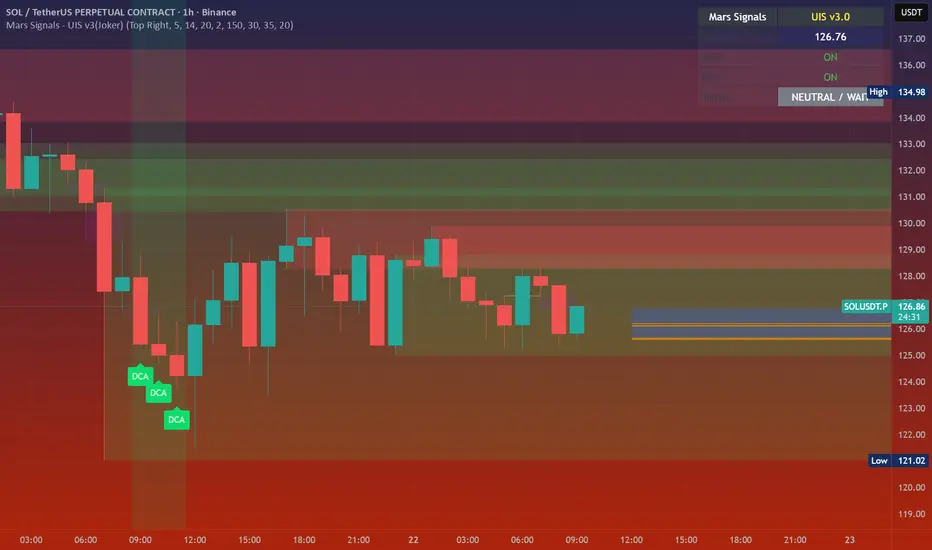
Lyapunov Market Instability (LMI)Lyapunov Market Instability (LMI)
What is Lyapunov Market Instability?
Lyapunov Market Instability (LMI) is a revolutionary indicator that brings chaos theory from theoretical physics into practical trading. By calculating Lyapunov exponents—a measure of how rapidly nearby trajectories diverge in phase space—LMI quantifies market sensitivity to initial conditions. This isn't another oscillator or trend indicator; it's a mathematical lens that reveals whether markets are in chaotic (trending) or stable (ranging) regimes.
Inspired by the meditative color field paintings of Mark Rothko, this indicator transforms complex chaos mathematics into an intuitive visual experience. The elegant simplicity of the visualization belies the sophisticated theory underneath—just as Rothko's seemingly simple color blocks contain profound depth.
Theoretical Foundation (Chaos Theory & Lyapunov Exponents)
In dynamical systems, the Lyapunov exponent (λ) measures the rate of separation of infinitesimally close trajectories:
λ > 0: System is chaotic—small changes lead to dramatically different outcomes (butterfly effect)
λ < 0: System is stable—trajectories converge, perturbations die out
λ ≈ 0: Edge of chaos—transition between regimes
Phase Space Reconstruction
Using Takens' embedding theorem , we reconstruct market dynamics in higher dimensions:
Time-delay embedding: Create vectors from price at different lags
Nearest neighbor search: Find historically similar market states
Trajectory evolution: Track how these similar states diverged over time
Divergence rate: Calculate average exponential separation
Market Application
Chaotic markets (λ > threshold): Strong trends emerge, momentum dominates, use breakout strategies
Stable markets (λ < threshold): Mean reversion dominates, fade extremes, range-bound strategies work
Transition zones: Market regime about to change, reduce position size, wait for confirmation
How LMI Works
1. Phase Space Construction
Each point in time is embedded as a vector using historical prices at specific delays (τ). This reveals the market's hidden attractor structure.
2. Lyapunov Calculation
For each current state, we:
- Find similar historical states within epsilon (ε) distance
- Track how these initially similar states evolved
- Measure exponential divergence rate
- Average across multiple trajectories for robustness
3. Signal Generation
Chaos signals: When λ crosses above threshold, market enters trending regime
Stability signals: When λ crosses below threshold, market enters ranging regime
Divergence detection: Price/Lyapunov divergences signal potential reversals
4. Rothko Visualization
Color fields: Background zones represent market states with Rothko-inspired palettes
Glowing line: Lyapunov exponent with intensity reflecting market state
Minimalist design: Focus on essential information without clutter
Inputs:
📐 Lyapunov Parameters
Embedding Dimension (default: 3)
Dimensions for phase space reconstruction
2-3: Simple dynamics (crypto/forex) - captures basic momentum patterns
4-5: Complex dynamics (stocks/indices) - captures intricate market structures
Higher dimensions need exponentially more data but reveal deeper patterns
Time Delay τ (default: 1)
Lag between phase space coordinates
1: High-frequency (1m-15m charts) - captures rapid market shifts
2-3: Medium frequency (1H-4H) - balances noise and signal
4-5: Low frequency (Daily+) - focuses on major regime changes
Match to your timeframe's natural cycle
Initial Separation ε (default: 0.001)
Neighborhood size for finding similar states
0.0001-0.0005: Highly liquid markets (major forex pairs)
0.0005-0.002: Normal markets (large-cap stocks)
0.002-0.01: Volatile markets (crypto, small-caps)
Smaller = more sensitive to chaos onset
Evolution Steps (default: 10)
How far to track trajectory divergence
5-10: Fast signals for scalping - quick regime detection
10-20: Balanced for day trading - reliable signals
20-30: Slow signals for swing trading - major regime shifts only
Nearest Neighbors (default: 5)
Phase space points for averaging
3-4: Noisy/fast markets - adapts quickly
5-6: Balanced (recommended) - smooth yet responsive
7-10: Smooth/slow markets - very stable signals
📊 Signal Parameters
Chaos Threshold (default: 0.05)
Lyapunov value above which market is chaotic
0.01-0.03: Sensitive - more chaos signals, earlier detection
0.05: Balanced - optimal for most markets
0.1-0.2: Conservative - only strong trends trigger
Stability Threshold (default: -0.05)
Lyapunov value below which market is stable
-0.01 to -0.03: Sensitive - quick stability detection
-0.05: Balanced - reliable ranging signals
-0.1 to -0.2: Conservative - only deep stability
Signal Smoothing (default: 3)
EMA period for noise reduction
1-2: Raw signals for experienced traders
3-5: Balanced - recommended for most
6-10: Very smooth for position traders
🎨 Rothko Visualization
Rothko Classic: Deep reds for chaos, midnight blues for stability
Orange/Red: Warm sunset tones throughout
Blue/Black: Cool, meditative ocean depths
Purple/Grey: Subtle, sophisticated palette
Visual Options:
Market Zones : Background fields showing regime areas
Transitions: Arrows marking regime changes
Divergences: Labels for price/Lyapunov divergences
Dashboard: Real-time state and trading signals
Guide: Educational panel explaining the theory
Visual Logic & Interpretation
Main Elements
Lyapunov Line: The heart of the indicator
Above chaos threshold: Market is trending, follow momentum
Below stability threshold: Market is ranging, fade extremes
Between thresholds: Transition zone, reduce risk
Background Zones: Rothko-inspired color fields
Red zone: Chaotic regime (trending)
Gray zone: Transition (uncertain)
Blue zone: Stable regime (ranging)
Transition Markers:
Up triangle: Entering chaos - start trend following
Down triangle: Entering stability - start mean reversion
Divergence Signals:
Bullish: Price makes low but Lyapunov rising (stability breaking down)
Bearish: Price makes high but Lyapunov falling (chaos dissipating)
Dashboard Information
Market State: Current regime (Chaotic/Stable/Transitioning)
Trading Bias: Specific strategy recommendation
Lyapunov λ: Raw value for precision
Signal Strength: Confidence in current regime
Last Change: Bars since last regime shift
Action: Clear trading directive
Trading Strategies
In Chaotic Regime (λ > threshold)
Follow trends aggressively: Breakouts have high success rate
Use momentum strategies: Moving average crossovers work well
Wider stops: Expect larger swings
Pyramid into winners: Trends tend to persist
In Stable Regime (λ < threshold)
Fade extremes: Mean reversion dominates
Use oscillators: RSI, Stochastic work well
Tighter stops: Smaller expected moves
Scale out at targets: Trends don't persist
In Transition Zone
Reduce position size: Uncertainty is high
Wait for confirmation: Let regime establish
Use options: Volatility strategies may work
Monitor closely: Quick changes possible
Advanced Techniques
- Multi-Timeframe Analysis
- Higher timeframe LMI for regime context
- Lower timeframe for entry timing
- Alignment = highest probability trades
- Divergence Trading
- Most powerful at regime boundaries
- Combine with support/resistance
- Use for early reversal detection
- Volatility Correlation
- Chaos often precedes volatility expansion
- Stability often precedes volatility contraction
- Use for options strategies
Originality & Innovation
LMI represents a genuine breakthrough in applying chaos theory to markets:
True Lyapunov Calculation: Not a simplified proxy but actual phase space reconstruction and divergence measurement
Rothko Aesthetic: Transforms complex math into meditative visual experience
Regime Detection: Identifies market state changes before price makes them obvious
Practical Application: Clear, actionable signals from theoretical physics
This is not a combination of existing indicators or a visual makeover of standard tools. It's a fundamental rethinking of how we measure and visualize market dynamics.
Best Practices
Start with defaults: Parameters are optimized for broad market conditions
Match to your timeframe: Adjust tau and evolution steps
Confirm with price action: LMI shows regime, not direction
Use appropriate strategies: Chaos = trend, Stability = reversion
Respect transitions: Reduce risk during regime changes
Alerts Available
Chaos Entry: Market entering chaotic regime - prepare for trends
Stability Entry: Market entering stable regime - prepare for ranges
Bullish Divergence: Potential bottom forming
Bearish Divergence: Potential top forming
Chart Information
Script Name: Lyapunov Market Instability (LMI) Recommended Use: All markets, all timeframes Best Performance: Liquid markets with clear regimes
Academic References
Takens, F. (1981). "Detecting strange attractors in turbulence"
Wolf, A. et al. (1985). "Determining Lyapunov exponents from a time series"
Rosenstein, M. et al. (1993). "A practical method for calculating largest Lyapunov exponents"
Note: After completing this indicator, I discovered @loxx's 2022 "Lyapunov Hodrick-Prescott Oscillator w/ DSL". While both explore Lyapunov exponents, they represent independent implementations with different methodologies and applications. This indicator uses phase space reconstruction for regime detection, while his combines Lyapunov concepts with HP filtering.
Disclaimer
This indicator is for research and educational purposes only. It does not constitute financial advice or provide direct buy/sell signals. Chaos theory reveals market character, not future prices. Always use proper risk management and combine with your own analysis. Past performance does not guarantee future results.
See markets through the lens of chaos. Trade the regime, not the noise.
Bringing theoretical physics to practical trading through the meditative aesthetics of Mark Rothko
Trade with insight. Trade with anticipation.
— Dskyz , for DAFE Trading Systems
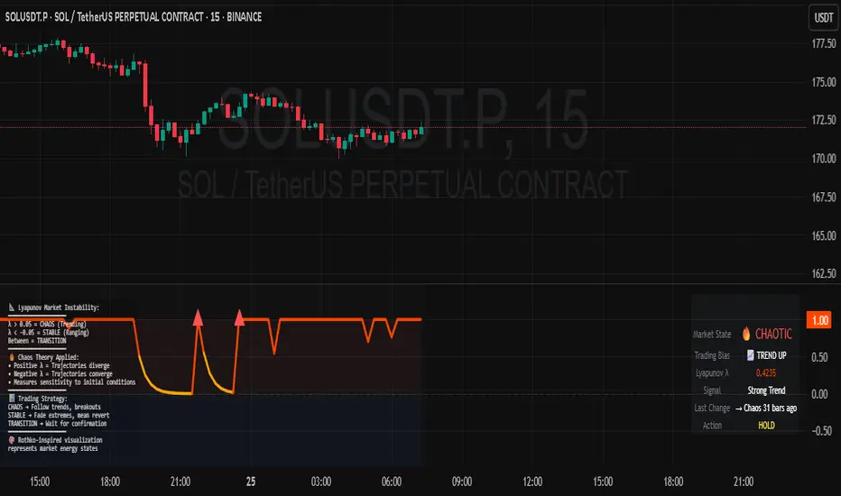
Optimus trader Optimus Trader
Indicator Description:
The Optimus Trader indicator is designed for technical traders looking for entry and exit points in financial markets. It combines signals based on volume, moving averages, VWAP (Volume Weighted Average Price), as well as the recognition of candlestick patterns such as Pin Bar and Inside Bars. This indicator helps identify opportune moments to buy or sell based on trends, volumes, and recent liquidity zones.
Parameters and Features:
1. Simple Moving Average (MA) and VWAP:
- Optimus Trader uses a 50-period simple moving average to determine the underlying trend. It also includes VWAP for precise price analysis based on traded volumes.
- These two indicators help identify whether the market is in an uptrend or downtrend, enhancing the reliability of buy and sell signals.
2. Volume :
- To avoid false signals, a volume threshold is set using a 20-period moving average, adjusted to 1.2 times the average volume. This filters signals by considering only high-volume periods, indicating heightened market interest.
3. Candlestick Pattern Recognition:
- Pin Bar: This sought-after candlestick pattern is detected for both bullish and bearish setups. A bullish or bearish *Pin Bar* often signals a possible reversal or continuation.
- *Inside Bar*: This price compression pattern is also detected, indicating a zone of indecision before a potential movement.
4. Trend:
- An uptrend is confirmed when the price is above the MA and VWAP, while a downtrend is identified when the price is below both indicators.
5. Liquidity Zones:
- Optimus Trader includes an approximate liquidity zone detection feature. By identifying recent support and resistance levels, the indicator detects if the price is near these zones. This feature strengthens the relevance of buy or sell signals.
6. Buy and Sell Signals:
- Buy: A buy signal is generated when the indicator detects a bullish *Pin Bar* or *Inside Bar* in an uptrend with high volume, and the price is close to a liquidity zone.
- Sell: A sell signal is generated when a bearish *Pin Bar* or *Inside Bar* is detected in a downtrend with high volume, and the price is near a liquidity zone.
Signal Display:
The signals are visible directly on the chart:
- A "BUY" label in green is displayed below the bar for buy signals.
- A "SELL" label in red is displayed above the bar for sell signals.
Summary:
This indicator is intended for traders seeking precise entry and exit points by integrating trend analysis, volume, and candlestick patterns. With liquidity zones, *Optimus Trader* helps minimize false signals, providing clear and accurate alerts.
---
This description can be directly added to TradingView to help users quickly understand the features and logic of this indicator.

Machine Learning: Support and Resistance [YinYangAlgorithms]Overview:
Support and Resistance is normally based upon Pivot Points and Highest Highs and Lowest Lows. Many times coders even incorporate Volume, RSI and other factors into the equation. However there may be a downside to doing a pure technical approach based on historical levels. We live in a time where Machine Learning is becoming more and more used; thus we have decided to create a Machine Learning Support and Resistance Projection based Indicator. Rather than using traditional Support and Resistance calculations using historical data, we have taken a rather different approach. This Indicator instead attempts to Predict and Project where Support and Resistance locations will be based on a Machine Learning Model using a form of KNN (k-Nearest Neighbors).
Since this indicator creates a Projection of where it deems Support and Resistance will be, it has the ability to move its Support and Resistance before the price even gets to it if it believes it will surpass its projections. This may create a more accurate placement of Support and Resistance as they’re not based on historical levels.
This Indicator does not Repaint.
How it works:
This Indicator makes its projections based on the source you provide (by default close) of the previous bar and submits the source, RSI and EMA to our Projection Function to get its projection of the current bar.
The Projection function essentially calculates potential movement after finding the differences between the source the MA from the current bar, previous bar and average over the span of Machine Learning Length.
Potential movement is defined as:
Average Difference + Average(Machine Learning Average, Average Last Distance)
Average Difference: (Absolute value of Current Source - Current MA) - (Absolute value of Machine Learning Average - Machine Learning MA)
Average Last Distance: Average(Current Source - Current MA, Previous Source - Previous MA)
It then predicts the next bars directional movement (bullish or bearish bar) using several factors:
Previous Source > Previous MA
Current Source - Current MA > Average Source - Average MA
Current RSI > Previous RSI
Current RSI > 30 and Previous RSI <= 30
Current RSI < 70 and Previous RSI >= 70
This helps us to predict the direction the next bar may move.
We then calculate a multiplier that we apply to our Potential Movement value to get our final result which is our Current Bars Close Projection.
Our multiplier is calculated using:
(Current RSI > 30 and Previous RSI <= 30) OR (Current RSI < 70 and Previous RSI >= 70)
Current Source - Current MA > Previous Source - Previous MA
We then create an array and fill it with the previous X projections (Machine Learning Length) and send it to another function. This function, if told to, will sort the data accordingly and then output the KNN average of the length given.
We calculate and plot various KNN lengths to create different Zones:
Strong Support: Length of 2 but sort the data Ascending (low to high)
Strong Resistance: Length of 2 but sort the data Descending (high to low)
Support: Length of Machine Length Length / 10 or Min of 2 sorted by Ascending
Resistance: Length of Machine Length Length / 10 or Min of 2 sorted by Descending
There are also 4 other plots you may be wondering what they are, there is your AVG, VWMA, Long Term Memory and Current Projection.
By default your Current Projection is disabled in settings but you can enable it if you are curious to see how the projections for each close are calculated. It is, however, not a crucial point of interest (white line).
The average is simply the average value of the Machine Learning Data (purple line).
The VWMA is a VWMA calculation applied to our Data over a length specified in settings (by default 1)(blue line). The VWMA is crucial when combined with the Avg as they can cross over and under each other. These crosses represent potential Bullish and Bearish zones.
Lastly, but certainly not least, we have the Long Term Memory (maroon line). The Long Term Memory can be displayed either as an ‘Average’, ‘Hard Line’ or ‘None’. The Long Term Average is only updated every Machine Learning Length Bar Index’s and is populated with the average of the Machine Learning Data. For Instance, if Machine Learning Length is set to 100, the Long Term Memory is only updated every 100 bars, and since its length is the same as the Machine Learning Length, that means its data is composed of 10,000 bars worth of data. The Long Term Memory may be very beneficial for determining where Support and Resistance lie over the Long Term within a Machine Learning Algorithm. When set to ‘Average’ it plots the connection lines diagonally, and although they may be more visually appealing, they’re less useful when it comes to actually seeing support and resistance as generally speaking, support and resistance lie on the horizontal. When set to ‘Hard Line’ the Long Term Memory is connected with hard lines and holds the price value until the next time it is updated. This makes it much more useful for potentially identifying Support and Resistance.
Tutorial:
Here is an overview of what the Indicator looks like, now let's start to dissect it.
In the example above we can see how all of the lines between the Major Support and Resistance zones may act as BOTH Support and Resistance depending on which side the price is currently on. In the circle on the left, we can see how it can fluctuate between the two. If you look at the circle on the right, we can see how the Average line acts as a strong support before it fails to maintain it. Generally speaking, most Support and Resistance locations may potentially fail to hold after 3 tests, as the Average did in this example.
As you can see, the Support and Resistance doesn’t wait to be tested before adjusting, which is why there are 2 lines which create their zones. The inner line is the Support/Resistance and the outer line is the Strong Support/Resistance. The Yellow Circle shows the inner line was able to calculate the moving resistance correctly and then adjusted accordingly as it was projecting the price to keep increasing. However, if you look at the White Circle, you can see that since there was first a crash, and then parabolic movement, that the inner zone could not move and predict the resistance as well as the outer zone could.
We consider the price to be ‘Overvalued’ when it is above the VWMA (blue line) and ‘Undervalued’ when it is below the VWMA. It is considered ‘fair’ price when it is within the VWMA to Average zone (between the blue and purple lines). If you look at the example above, you’ll notice where the two yellow circles are, it is not only considered ‘Overvalued’, but it then proceeds to ride the inner resistance line upwards. This is common when the market is overly bullish and vice versa when it is bearish. Please keep in mind, although it is common, it doesn’t mean a correction can’t happen.
In this example above we look at the last bull run that may have started due to the halving. This bull run was very bullish as you can see in the example above. The price was constantly sitting within the Resistance Zone and the VWMA that was very close to it was constantly acting as a Support. Naturally, due to the Algorithm used in this Indicator, as the momentum starts to slow down, the VWMA (blue line) will start to space out more and more from the Resistance Zone. This doesn’t mean the momentum is gone, it just means it may be slowing down.
Unfortunately we have to study the Bear Market with a different perspective than the Bull Market. However, there are still some similarities within the two. If you refer to the example above and the previous example, you can clearly see that the Bull Market loves to stay with the Resistance Zone and use the VWMA as a Support. However, the Bear Market does not. This is a normal occurrence, however we can see from the example above you may see a correction / horizontal movement when the Outer Support Line is touched. If you look at all 3 yellow circles, the Outer Support Line was touched, then either a small correction or horizontal consolidation occurred.
We will conclude our Tutorial here, hopefully you’ll be able to benefit from a moving Support and Resistance calculated with Machine Learning that projects its locations, rather than using traditional calculations.
Settings:
Source: This source is the base for all our calculations
Machine Learning Length: How much projection data are we storing and using to make calculations.
Smoothing Length: We need to smooth calculations such as RSI, EMA and VWMA. What length are we smoothing it with?
VWMA ML Projection Length: How far into our Machine Learning data should we average for our VWMA. Please note the 'Smoothing Length' is still applied here after getting the Projection Average.
Long Term Memory: Long term memory has the same storage length but is only updated once per Machine Learning Length. For instance, if Machine Learning Length is 100, it will save the Average of our data once every 100 bars. This means its memory is an average of 10,000 bars of Machine Learning. 'Average' connects its values diagonally whereas 'Hard Line' holds its value until it changes.
Use Average Last Distance In Potential Movement: This can help accuracy but generally also displaces the Support and Resistance by projecting it further.
Show Current Projection: Projections occur for each bar, and our Machine Learning utilizes these projections by storing and evaluating them. This toggle will display the Current Projection Line which is used to create all our Projections.
If you have any questions, comments, ideas or concerns please don't hesitate to contact us.
HAPPY TRADING!
Reverse Cutlers Relative Strength Index On ChartIntroduction
The Reverse Cutlers Relative Strength Index (RCRSI) OC is an indicator which tells the user what price is required to give a particular Cutlers Relative Strength Index ( RSI ) value, or cross its Moving Average (MA) signal line.
Overview
Background & Credits:
The relative strength index ( RSI ) is a momentum indicator used in technical analysis that was originally developed by J. Welles Wilder Jr. and introduced in his seminal 1978 book, “New Concepts in Technical Trading Systems.”.
Cutler created a variation of the RSI known as “Cutlers RSI” using a different formulation to avoid an inherent accuracy problem which arises when using Wilders method of smoothing.
Further developments in the use, and more nuanced interpretations of the RSI have been developed by Cardwell, and also by well-known chartered market technician, Constance Brown C.M.T., in her acclaimed book "Technical Analysis for the Trading Professional” 1999 where she described the idea of bull and bear market ranges for RSI , and while she did not actually reveal the formulas, she introduced the concept of “reverse engineering” the RSI to give price level outputs.
Renowned financial software developer, co-author of academic books on finance, and scientific fellow to the Department of Finance and Insurance at the Technological Educational Institute of Crete, Giorgos Siligardos PHD . brought a new perspective to Wilder’s RSI when he published his excellent and well-received articles "Reverse Engineering RSI " and "Reverse Engineering RSI II " in the June 2003, and August 2003 issues of Stocks & Commodities magazine, where he described his methods of reverse engineering Wilders RSI .
Several excellent Implementations of the Reverse Wilders Relative Strength Index have been published here on Tradingview and elsewhere.
My utmost respect, and all due credits to authors of related prior works.
Introduction
It is worth noting that while the general RSI formula, and the logic dictating the UpMove and DownMove data series has remained the same as the Wilders original formulation, it has been interpreted in a different way by using a different method of averaging the upward, and downward moves.
Cutler recognized the issue of data length dependency when using wilders smoothing method of calculating RSI which means that wilders standard RSI will have a potential initialization error which reduces with every new data point calculated meaning early results should be regarded as unreliable until enough calculation iterations have occurred for convergence.
Hence Cutler proposed using Simple Moving Averaging for gain and loss data which this Indicator is based on.
Having "Reverse engineered" prices for any oscillator makes the planning, and execution of strategies around that oscillator far simpler, more timely and effective.
Introducing the Reverse Cutlers RSI which consists of plotted lines on a scale of 0 to 100, and an optional infobox.
The RSI scale is divided into zones:
• Scale high (100)
• Bull critical zone (80 - 100)
• Bull control zone (62 - 80)
• Scale midline (50)
• Bear control zone (20 - 38)
• Bear critical zone (0 - 20)
• Scale low (0)
The RSI plots which graphically display output closing price levels where Cutlers RSI value will crossover:
• RSI (eq) (previous RSI value)
• RSI MA signal line
• RSI Test price
• Alert level high
• Alert level low
The info box displays output closing price levels where Cutlers RSI value will crossover:
• Its previous value. ( RSI )
• Bull critical zone.
• Bull control zone.
• Mid-Line.
• Bear control zone.
• Bear critical zone.
• RSI MA signal line
• Alert level High
• Alert level low
And also displays the resultant RSI for a user defined closing price:
• Test price RSI
The infobox outputs can be shown for the current bar close, or the next bar close.
The user can easily select which information they want in the infobox from the setttings
Importantly:
All info box price levels for the current bar are calculated immediately upon the current bar closing and a new bar opening, they will not change until the current bar closes.
All info box price levels for the next bar are projections which are continually recalculated as the current price changes, and therefore fluctuate as the current price changes.
Understanding the Relative Strength Index
At its simplest the RSI is a measure of how quickly traders are bidding the price of an asset up or down.
It does this by calculating the difference in magnitude of price gains and losses over a specific lookback period to evaluate market conditions.
The RSI is displayed as an oscillator (a line graph that can move between two extremes) and outputs a value limited between 0 and 100.
It is typically accompanied by a moving average signal line.
Traditional interpretations
Overbought and oversold:
An RSI value of 70 or above indicates that an asset is becoming overbought (overvalued condition), and may be may be ready for a trend reversal or corrective pullback in price.
An RSI value of 30 or below indicates that an asset is becoming oversold (undervalued condition), and may be may be primed for a trend reversal or corrective pullback in price.
Midline Crossovers:
When the RSI crosses above its midline ( RSI > 50%) a bullish bias signal is generated. (only take long trades)
When the RSI crosses below its midline ( RSI < 50%) a bearish bias signal is generated. (only take short trades)
Bullish and bearish moving average signal Line crossovers:
When the RSI line crosses above its signal line, a bullish buy signal is generated
When the RSI line crosses below its signal line, a bearish sell signal is generated.
Swing Failures and classic rejection patterns:
If the RSI makes a lower high, and then follows with a downside move below the previous low, a Top Swing Failure has occurred.
If the RSI makes a higher low, and then follows with an upside move above the previous high, a Bottom Swing Failure has occurred.
Examples of classic swing rejection patterns
Bullish swing rejection pattern:
The RSI moves into oversold zone (below 30%).
The RSI rejects back out of the oversold zone (above 30%)
The RSI forms another dip without crossing back into oversold zone.
The RSI then continues the bounce to break up above the previous high.
Bearish swing rejection pattern:
The RSI moves into overbought zone (above 70%).
The RSI rejects back out of the overbought zone (below 70%)
The RSI forms another peak without crossing back into overbought zone.
The RSI then continues to break down below the previous low.
Divergences:
A regular bullish RSI divergence is when the price makes lower lows in a downtrend and the RSI indicator makes higher lows.
A regular bearish RSI divergence is when the price makes higher highs in an uptrend and the RSI indicator makes lower highs.
A hidden bullish RSI divergence is when the price makes higher lows in an uptrend and the RSI indicator makes lower lows.
A hidden bearish RSI divergence is when the price makes lower highs in a downtrend and the RSI indicator makes higher highs.
Regular divergences can signal a reversal of the trending direction.
Hidden divergences can signal a continuation in the direction of the trend.
Chart Patterns:
RSI regularly forms classic chart patterns that may not show on the underlying price chart, such as ascending and descending triangles & wedges , double tops, bottoms and trend lines etc.
Support and Resistance:
It is very often easier to define support or resistance levels on the RSI itself rather than the price chart.
Modern interpretations in trending markets:
Modern interpretations of the RSI stress the context of the greater trend when using RSI signals such as crossovers, overbought/oversold conditions, divergences and patterns.
Constance Brown, CMT , was one of the first who promoted the idea that an oversold reading on the RSI in an uptrend is likely much higher than 30%, and that an overbought reading on the RSI during a downtrend is much lower than the 70% level.
In an uptrend or bull market, the RSI tends to remain in the 40 to 90 range, with the 40-50 zone acting as support.
During a downtrend or bear market, the RSI tends to stay between the 10 to 60 range, with the 50-60 zone acting as resistance.
For ease of executing more modern and nuanced interpretations of RSI it is very useful to break the RSI scale into bull and bear control and critical zones.
These ranges will vary depending on the RSI settings and the strength of the specific market’s underlying trend.
Limitations of the RSI
Like most technical indicators, its signals are most reliable when they conform to the long-term trend.
True trend reversal signals are rare, and can be difficult to separate from false signals.
False signals or “fake-outs”, e.g. a bullish crossover, followed by a sudden decline in price, are common.
Since the indicator displays momentum, it can stay overbought or oversold for a long time when an asset has significant sustained momentum in either direction.
Data Length Dependency when using wilders smoothing method of calculating RSI means that wilders standard RSI will have a potential initialization error which reduces with every new data point calculated meaning early results should be regarded as unreliable until calculation iterations have occurred for convergence.

Reverse Cutlers Relative Strength IndexIntroduction
The Reverse Cutlers Relative Strength Index (RCRSI) is an indicator which tells the user what price is required to give a particular Cutlers Relative Strength Index (RSI) value, or cross its Moving Average (MA) signal line.
Overview
Background & Credits:
The relative strength index (RSI) is a momentum indicator used in technical analysis that was originally developed by J. Welles Wilder Jr. and introduced in his seminal 1978 book, “New Concepts in Technical Trading Systems.”.
Cutler created a variation of the RSI known as “Cutlers RSI” using a different formulation to avoid an inherent accuracy problem which arises when using Wilders method of smoothing.
Further developments in the use, and more nuanced interpretations of the RSI have been developed by Cardwell, and also by well-known chartered market technician, Constance Brown C.M.T., in her acclaimed book "Technical Analysis for the Trading Professional” 1999 where she described the idea of bull and bear market ranges for RSI, and while she did not actually reveal the formulas, she introduced the concept of “reverse engineering” the RSI to give price level outputs.
Renowned financial software developer, co-author of academic books on finance, and scientific fellow to the Department of Finance and Insurance at the Technological Educational Institute of Crete, Giorgos Siligardos PHD. brought a new perspective to Wilder’s RSI when he published his excellent and well-received articles "Reverse Engineering RSI " and "Reverse Engineering RSI II " in the June 2003, and August 2003 issues of Stocks & Commodities magazine, where he described his methods of reverse engineering Wilders RSI.
Several excellent Implementations of the Reverse Wilders Relative Strength Index have been published here on Tradingview and elsewhere.
My utmost respect, and all due credits to authors of related prior works.
Introduction
It is worth noting that while the general RSI formula, and the logic dictating the UpMove and DownMove data series as described above has remained the same as the Wilders original formulation, it has been interpreted in a different way by using a different method of averaging the upward, and downward moves.
Cutler recognized the issue of data length dependency when using wilders smoothing method of calculating RSI which means that wilders standard RSI will have a potential initialization error which reduces with every new data point calculated meaning early results should be regarded as unreliable until enough calculation iterations have occurred for convergence.
Hence Cutler proposed using Simple Moving Averaging for gain and loss data which this Indicator is based on.
Having "Reverse engineered" prices for any oscillator makes the planning, and execution of strategies around that oscillator far simpler, more timely and effective.
Introducing the Reverse Cutlers RSI which consists of plotted lines on a scale of 0 to 100, and an optional infobox.
The RSI scale is divided into zones:
• Scale high (100)
• Bull critical zone (80 - 100)
• Bull control zone (62 - 80)
• Scale midline (50)
• Bear critical zone (20 - 38)
• Bear control zone (0 - 20)
• Scale low (0)
The RSI plots are:
• Cutlers RSI
• RSI MA signal line
• Test price RSI
• Alert level high
• Alert level low
The info box displays output closing price levels where Cutlers RSI value will crossover:
• Its previous value. (RSI )
• Bull critical zone.
• Bull control zone.
• Mid-Line.
• Bear control zone.
• Bear critical zone.
• RSI MA signal line
• Alert level High
• Alert level low
And also displays the resultant RSI for a user defined closing price:
• Test price RSI
The infobox outputs can be shown for the current bar close, or the next bar close.
The user can easily select which information they want in the infobox from the setttings
Importantly:
All info box price levels for the current bar are calculated immediately upon the current bar closing and a new bar opening, they will not change until the current bar closes.
All info box price levels for the next bar are projections which are continually recalculated as the current price changes, and therefore fluctuate as the current price changes.
Understanding the Relative Strength Index
At its simplest the RSI is a measure of how quickly traders are bidding the price of an asset up or down.
It does this by calculating the difference in magnitude of price gains and losses over a specific lookback period to evaluate market conditions.
The RSI is displayed as an oscillator (a line graph that can move between two extremes) and outputs a value limited between 0 and 100.
It is typically accompanied by a moving average signal line.
Traditional interpretations
Overbought and oversold:
An RSI value of 70 or above indicates that an asset is becoming overbought (overvalued condition), and may be may be ready for a trend reversal or corrective pullback in price.
An RSI value of 30 or below indicates that an asset is becoming oversold (undervalued condition), and may be may be primed for a trend reversal or corrective pullback in price.
Midline Crossovers:
When the RSI crosses above its midline (RSI > 50%) a bullish bias signal is generated. (only take long trades)
When the RSI crosses below its midline (RSI < 50%) a bearish bias signal is generated. (only take short trades)
Bullish and bearish moving average signal Line crossovers:
When the RSI line crosses above its signal line, a bullish buy signal is generated
When the RSI line crosses below its signal line, a bearish sell signal is generated.
Swing Failures and classic rejection patterns:
If the RSI makes a lower high, and then follows with a downside move below the previous low, a Top Swing Failure has occurred.
If the RSI makes a higher low, and then follows with an upside move above the previous high, a Bottom Swing Failure has occurred.
Examples of classic swing rejection patterns
Bullish swing rejection pattern:
The RSI moves into oversold zone (below 30%).
The RSI rejects back out of the oversold zone (above 30%)
The RSI forms another dip without crossing back into oversold zone.
The RSI then continues the bounce to break up above the previous high.
Bearish swing rejection pattern:
The RSI moves into overbought zone (above 70%).
The RSI rejects back out of the overbought zone (below 70%)
The RSI forms another peak without crossing back into overbought zone.
The RSI then continues to break down below the previous low.
Divergences:
A regular bullish RSI divergence is when the price makes lower lows in a downtrend and the RSI indicator makes higher lows.
A regular bearish RSI divergence is when the price makes higher highs in an uptrend and the RSI indicator makes lower highs.
A hidden bullish RSI divergence is when the price makes higher lows in an uptrend and the RSI indicator makes lower lows.
A hidden bearish RSI divergence is when the price makes lower highs in a downtrend and the RSI indicator makes higher highs.
Regular divergences can signal a reversal of the trending direction.
Hidden divergences can signal a continuation in the direction of the trend.
Chart Patterns:
RSI regularly forms classic chart patterns that may not show on the underlying price chart, such as ascending and descending triangles & wedges, double tops, bottoms and trend lines etc.
Support and Resistance:
It is very often easier to define support or resistance levels on the RSI itself rather than the price chart.
Modern interpretations in trending markets:
Modern interpretations of the RSI stress the context of the greater trend when using RSI signals such as crossovers, overbought/oversold conditions, divergences and patterns.
Constance Brown, CMT, was one of the first who promoted the idea that an oversold reading on the RSI in an uptrend is likely much higher than 30%, and that an overbought reading on the RSI during a downtrend is much lower than the 70% level.
In an uptrend or bull market, the RSI tends to remain in the 40 to 90 range, with the 40-50 zone acting as support.
During a downtrend or bear market, the RSI tends to stay between the 10 to 60 range, with the 50-60 zone acting as resistance.
For ease of executing more modern and nuanced interpretations of RSI it is very useful to break the RSI scale into bull and bear control and critical zones.
These ranges will vary depending on the RSI settings and the strength of the specific market’s underlying trend.
Limitations of the RSI
Like most technical indicators, its signals are most reliable when they conform to the long-term trend.
True trend reversal signals are rare, and can be difficult to separate from false signals.
False signals or “fake-outs”, e.g. a bullish crossover, followed by a sudden decline in price, are common.
Since the indicator displays momentum, it can stay overbought or oversold for a long time when an asset has significant sustained momentum in either direction.
Data Length Dependency when using wilders smoothing method of calculating RSI means that wilders standard RSI will have a potential initialization error which reduces with every new data point calculated meaning early results should be regarded as unreliable until calculation iterations have occurred for convergence.
RSI Statistics [Honestcowboy]⯁ Overview
Research tool for analysing price behaviour based on RSI, find out how your favorite trading pair / timeframe combinations react to RSI. 5 Different projections based on 5 different value zones of RSI:
RSI between 100-80 (very overbought)
RSI between 80-60 (overbought)
RSI between 60-40 (normal)
RSI between 40-20 (oversold)
RSI between 20-00 (very oversold)
The script simply show price projections of different RSI environments so you can get an idea of what price could do when RSI reaches this RSI value zone. Ofcourse past price performance does not guarantee future returns and this is just projections based on the past.
The script also projects RSI just like it does with price so you can get an idea of how long RSI might stay in overbought or very overbought etc
Script is mainly a research tool to use to get ideas to explore further and build upon. Here are some examples:
⯁ Settings
RSI Lenght: this is just normal RSI settings you find in standard RSI (bars used to calculate RSI)
Projection Length: Amount of bars to save for projections. The projections will also project this many bars in futre. Higher values here increase loading time drastically.
Price Action Boundaries: turn the highs / lows of projection zone on or off. I usually turn this off to look more closely at the averages themselves.
Maximum Stats history: Not on by default, in case you only want to show the average projection of last X amount of occurences RSI was in a specific RSI value zone
Selection of the different zones: in case you want to look at a specific zone alone or turn of some zones. It will no longer project for that zone both in the price projection and RSI projections.
⯁ How are these calculated?
To calculate the average price reaction script uses a very simple approach. On each bar it will save price action array up to projection length back in time. It will then check what the RSI value was there and store the array inside the right matrix.
It will use this matrix to calculate the averages, highs and lows of all these arrays for that specific RSI zone. It uses a simple arithmatic averaging method to get average value.
The script uses a similar approach for projecting the RSI itself into the future.
I include a visual showing it a bit better. This is from a different indicator of me using same approach:
The script will force you into a specific background, bar color and color template. Script is not meant to be used with other scripts and should be used as a standalone tool.

Adaptive Market Wave TheoryAdaptive Market Wave Theory
🌊 CORE INNOVATION: PROBABILISTIC PHASE DETECTION WITH MULTI-AGENT CONSENSUS
Adaptive Market Wave Theory (AMWT) represents a fundamental paradigm shift in how traders approach market phase identification. Rather than counting waves subjectively or drawing static breakout levels, AMWT treats the market as a hidden state machine —using Hidden Markov Models, multi-agent consensus systems, and reinforcement learning algorithms to quantify what traditional methods leave to interpretation.
The Wave Analysis Problem:
Traditional wave counting methodologies (Elliott Wave, harmonic patterns, ABC corrections) share fatal weaknesses that AMWT directly addresses:
1. Non-Falsifiability : Invalid wave counts can always be "recounted" or "adjusted." If your Wave 3 fails, it becomes "Wave 3 of a larger degree" or "actually Wave C." There's no objective failure condition.
2. Observer Bias : Two expert wave analysts examining the same chart routinely reach different conclusions. This isn't a feature—it's a fundamental methodology flaw.
3. No Confidence Measure : Traditional analysis says "This IS Wave 3." But with what probability? 51%? 95%? The binary nature prevents proper position sizing and risk management.
4. Static Rules : Fixed Fibonacci ratios and wave guidelines cannot adapt to changing market regimes. What worked in 2019 may fail in 2024.
5. No Accountability : Wave methodologies rarely track their own performance. There's no feedback loop to improve.
The AMWT Solution:
AMWT addresses each limitation through rigorous mathematical frameworks borrowed from speech recognition, machine learning, and reinforcement learning:
• Non-Falsifiability → Hard Invalidation : Wave hypotheses die permanently when price violates calculated invalidation levels. No recounting allowed.
• Observer Bias → Multi-Agent Consensus : Three independent analytical agents must agree. Single-methodology bias is eliminated.
• No Confidence → Probabilistic States : Every market state has a calculated probability from Hidden Markov Model inference. "72% probability of impulse state" replaces "This is Wave 3."
• Static Rules → Adaptive Learning : Thompson Sampling multi-armed bandits learn which agents perform best in current conditions. The system adapts in real-time.
• No Accountability → Performance Tracking : Comprehensive statistics track every signal's outcome. The system knows its own performance.
The Core Insight:
"Traditional wave analysis asks 'What count is this?' AMWT asks 'What is the probability we are in an impulsive state, with what confidence, confirmed by how many independent methodologies, and anchored to what liquidity event?'"
🔬 THEORETICAL FOUNDATION: HIDDEN MARKOV MODELS
Why Hidden Markov Models?
Markets exist in hidden states that we cannot directly observe—only their effects on price are visible. When the market is in an "impulse up" state, we see rising prices, expanding volume, and trending indicators. But we don't observe the state itself—we infer it from observables.
This is precisely the problem Hidden Markov Models (HMMs) solve. Originally developed for speech recognition (inferring words from sound waves), HMMs excel at estimating hidden states from noisy observations.
HMM Components:
1. Hidden States (S) : The unobservable market conditions
2. Observations (O) : What we can measure (price, volume, indicators)
3. Transition Matrix (A) : Probability of moving between states
4. Emission Matrix (B) : Probability of observations given each state
5. Initial Distribution (π) : Starting state probabilities
AMWT's Six Market States:
State 0: IMPULSE_UP
• Definition: Strong bullish momentum with high participation
• Observable Signatures: Rising prices, expanding volume, RSI >60, price above upper Bollinger Band, MACD histogram positive and rising
• Typical Duration: 5-20 bars depending on timeframe
• What It Means: Institutional buying pressure, trend acceleration phase
State 1: IMPULSE_DN
• Definition: Strong bearish momentum with high participation
• Observable Signatures: Falling prices, expanding volume, RSI <40, price below lower Bollinger Band, MACD histogram negative and falling
• Typical Duration: 5-20 bars (often shorter than bullish impulses—markets fall faster)
• What It Means: Institutional selling pressure, panic or distribution acceleration
State 2: CORRECTION
• Definition: Counter-trend consolidation with declining momentum
• Observable Signatures: Sideways or mild counter-trend movement, contracting volume, RSI returning toward 50, Bollinger Bands narrowing
• Typical Duration: 8-30 bars
• What It Means: Profit-taking, digestion of prior move, potential accumulation for next leg
State 3: ACCUMULATION
• Definition: Base-building near lows where informed participants absorb supply
• Observable Signatures: Price near recent lows but not making new lows, volume spikes on up bars, RSI showing positive divergence, tight range
• Typical Duration: 15-50 bars
• What It Means: Smart money buying from weak hands, preparing for markup phase
State 4: DISTRIBUTION
• Definition: Top-forming near highs where informed participants distribute holdings
• Observable Signatures: Price near recent highs but struggling to advance, volume spikes on down bars, RSI showing negative divergence, widening range
• Typical Duration: 15-50 bars
• What It Means: Smart money selling to late buyers, preparing for markdown phase
State 5: TRANSITION
• Definition: Regime change period with mixed signals and elevated uncertainty
• Observable Signatures: Conflicting indicators, whipsaw price action, no clear momentum, high volatility without direction
• Typical Duration: 5-15 bars
• What It Means: Market deciding next direction, dangerous for directional trades
The Transition Matrix:
The transition matrix A captures the probability of moving from one state to another. AMWT initializes with empirically-derived values then updates online:
From/To IMP_UP IMP_DN CORR ACCUM DIST TRANS
IMP_UP 0.70 0.02 0.20 0.02 0.04 0.02
IMP_DN 0.02 0.70 0.20 0.04 0.02 0.02
CORR 0.15 0.15 0.50 0.10 0.10 0.00
ACCUM 0.30 0.05 0.15 0.40 0.05 0.05
DIST 0.05 0.30 0.15 0.05 0.40 0.05
TRANS 0.20 0.20 0.20 0.15 0.15 0.10
Key Insights from Transition Probabilities:
• Impulse states are sticky (70% self-transition): Once trending, markets tend to continue
• Corrections can transition to either impulse direction (15% each): The next move after correction is uncertain
• Accumulation strongly favors IMP_UP transition (30%): Base-building leads to rallies
• Distribution strongly favors IMP_DN transition (30%): Topping leads to declines
The Viterbi Algorithm:
Given a sequence of observations, how do we find the most likely state sequence? This is the Viterbi algorithm—dynamic programming to find the optimal path through the state space.
Mathematical Formulation:
δ_t(j) = max_i × B_j(O_t)
Where:
δ_t(j) = probability of most likely path ending in state j at time t
A_ij = transition probability from state i to state j
B_j(O_t) = emission probability of observation O_t given state j
AMWT Implementation:
AMWT runs Viterbi over a rolling window (default 50 bars), computing the most likely state sequence and extracting:
• Current state estimate
• State confidence (probability of current state vs alternatives)
• State sequence for pattern detection
Online Learning (Baum-Welch Adaptation):
Unlike static HMMs, AMWT continuously updates its transition and emission matrices based on observed market behavior:
f_onlineUpdateHMM(prev_state, curr_state, observation, decay) =>
// Update transition matrix
A *= decay
A += (1.0 - decay)
// Renormalize row
// Update emission matrix
B *= decay
B += (1.0 - decay)
// Renormalize row
The decay parameter (default 0.85) controls adaptation speed:
• Higher decay (0.95): Slower adaptation, more stable, better for consistent markets
• Lower decay (0.80): Faster adaptation, more reactive, better for regime changes
Why This Matters for Trading:
Traditional indicators give you a number (RSI = 72). AMWT gives you a probabilistic state assessment :
"There is a 78% probability we are in IMPULSE_UP state, with 15% probability of CORRECTION and 7% distributed among other states. The transition matrix suggests 70% chance of remaining in IMPULSE_UP next bar, 20% chance of transitioning to CORRECTION."
This enables:
• Position sizing by confidence : 90% confidence = full size; 60% confidence = half size
• Risk management by transition probability : High correction probability = tighten stops
• Strategy selection by state : IMPULSE = trend-follow; CORRECTION = wait; ACCUMULATION = scale in
🎰 THE 3-BANDIT CONSENSUS SYSTEM
The Multi-Agent Philosophy:
No single analytical methodology works in all market conditions. Trend-following excels in trending markets but gets chopped in ranges. Mean-reversion excels in ranges but gets crushed in trends. Structure-based analysis works when structure is clear but fails in chaotic markets.
AMWT's solution: employ three independent agents , each analyzing the market from a different perspective, then use Thompson Sampling to learn which agents perform best in current conditions.
Agent 1: TREND AGENT
Philosophy : Markets trend. Follow the trend until it ends.
Analytical Components:
• EMA Alignment: EMA8 > EMA21 > EMA50 (bullish) or inverse (bearish)
• MACD Histogram: Direction and rate of change
• Price Momentum: Close relative to ATR-normalized movement
• VWAP Position: Price above/below volume-weighted average price
Signal Generation:
Strong Bull: EMA aligned bull AND MACD histogram > 0 AND momentum > 0.3 AND close > VWAP
→ Signal: +1 (Long), Confidence: 0.75 + |momentum| × 0.4
Moderate Bull: EMA stack bull AND MACD rising AND momentum > 0.1
→ Signal: +1 (Long), Confidence: 0.65 + |momentum| × 0.3
Strong Bear: EMA aligned bear AND MACD histogram < 0 AND momentum < -0.3 AND close < VWAP
→ Signal: -1 (Short), Confidence: 0.75 + |momentum| × 0.4
Moderate Bear: EMA stack bear AND MACD falling AND momentum < -0.1
→ Signal: -1 (Short), Confidence: 0.65 + |momentum| × 0.3
When Trend Agent Excels:
• Trend days (IB extension >1.5x)
• Post-breakout continuation
• Institutional accumulation/distribution phases
When Trend Agent Fails:
• Range-bound markets (ADX <20)
• Chop zones after volatility spikes
• Reversal days at major levels
Agent 2: REVERSION AGENT
Philosophy: Markets revert to mean. Extreme readings reverse.
Analytical Components:
• Bollinger Band Position: Distance from bands, percent B
• RSI Extremes: Overbought (>70) and oversold (<30)
• Stochastic: %K/%D crossovers at extremes
• Band Squeeze: Bollinger Band width contraction
Signal Generation:
Oversold Bounce: BB %B < 0.20 AND RSI < 35 AND Stochastic < 25
→ Signal: +1 (Long), Confidence: 0.70 + (30 - RSI) × 0.01
Overbought Fade: BB %B > 0.80 AND RSI > 65 AND Stochastic > 75
→ Signal: -1 (Short), Confidence: 0.70 + (RSI - 70) × 0.01
Squeeze Fire Bull: Band squeeze ending AND close > upper band
→ Signal: +1 (Long), Confidence: 0.65
Squeeze Fire Bear: Band squeeze ending AND close < lower band
→ Signal: -1 (Short), Confidence: 0.65
When Reversion Agent Excels:
• Rotation days (price stays within IB)
• Range-bound consolidation
• After extended moves without pullback
When Reversion Agent Fails:
• Strong trend days (RSI can stay overbought for days)
• Breakout moves
• News-driven directional moves
Agent 3: STRUCTURE AGENT
Philosophy: Market structure reveals institutional intent. Follow the smart money.
Analytical Components:
• Break of Structure (BOS): Price breaks prior swing high/low
• Change of Character (CHOCH): First break against prevailing trend
• Higher Highs/Higher Lows: Bullish structure
• Lower Highs/Lower Lows: Bearish structure
• Liquidity Sweeps: Stop runs that reverse
Signal Generation:
BOS Bull: Price breaks above prior swing high with momentum
→ Signal: +1 (Long), Confidence: 0.70 + structure_strength × 0.2
CHOCH Bull: First higher low after downtrend, breaking structure
→ Signal: +1 (Long), Confidence: 0.75
BOS Bear: Price breaks below prior swing low with momentum
→ Signal: -1 (Short), Confidence: 0.70 + structure_strength × 0.2
CHOCH Bear: First lower high after uptrend, breaking structure
→ Signal: -1 (Short), Confidence: 0.75
Liquidity Sweep Long: Price sweeps below swing low then reverses strongly
→ Signal: +1 (Long), Confidence: 0.80
Liquidity Sweep Short: Price sweeps above swing high then reverses strongly
→ Signal: -1 (Short), Confidence: 0.80
When Structure Agent Excels:
• After liquidity grabs (stop runs)
• At major swing points
• During institutional accumulation/distribution
When Structure Agent Fails:
• Choppy, structureless markets
• During news events (structure becomes noise)
• Very low timeframes (noise overwhelms structure)
Thompson Sampling: The Bandit Algorithm
With three agents giving potentially different signals, how do we decide which to trust? This is the multi-armed bandit problem —balancing exploitation (using what works) with exploration (testing alternatives).
Thompson Sampling Solution:
Each agent maintains a Beta distribution representing its success/failure history:
Agent success rate modeled as Beta(α, β)
Where:
α = number of successful signals + 1
β = number of failed signals + 1
On Each Bar:
1. Sample from each agent's Beta distribution
2. Weight agent signals by sampled probabilities
3. Combine weighted signals into consensus
4. Update α/β based on trade outcomes
Mathematical Implementation:
// Beta sampling via Gamma ratio method
f_beta_sample(alpha, beta) =>
g1 = f_gamma_sample(alpha)
g2 = f_gamma_sample(beta)
g1 / (g1 + g2)
// Thompson Sampling selection
for each agent:
sampled_prob = f_beta_sample(agent.alpha, agent.beta)
weight = sampled_prob / sum(all_sampled_probs)
consensus += agent.signal × agent.confidence × weight
Why Thompson Sampling?
• Automatic Exploration : Agents with few samples get occasional chances (high variance in Beta distribution)
• Bayesian Optimal : Mathematically proven optimal solution to exploration-exploitation tradeoff
• Uncertainty-Aware : Small sample size = more exploration; large sample size = more exploitation
• Self-Correcting : Poor performers naturally get lower weights over time
Example Evolution:
Day 1 (Initial):
Trend Agent: Beta(1,1) → samples ~0.50 (high uncertainty)
Reversion Agent: Beta(1,1) → samples ~0.50 (high uncertainty)
Structure Agent: Beta(1,1) → samples ~0.50 (high uncertainty)
After 50 Signals:
Trend Agent: Beta(28,23) → samples ~0.55 (moderate confidence)
Reversion Agent: Beta(18,33) → samples ~0.35 (underperforming)
Structure Agent: Beta(32,19) → samples ~0.63 (outperforming)
Result: Structure Agent now receives highest weight in consensus
Consensus Requirements by Mode:
Aggressive Mode:
• Minimum 1/3 agents agreeing
• Consensus threshold: 45%
• Use case: More signals, higher risk tolerance
Balanced Mode:
• Minimum 2/3 agents agreeing
• Consensus threshold: 55%
• Use case: Standard trading
Conservative Mode:
• Minimum 2/3 agents agreeing
• Consensus threshold: 65%
• Use case: Higher quality, fewer signals
Institutional Mode:
• Minimum 2/3 agents agreeing
• Consensus threshold: 75%
• Additional: Session quality >0.65, mode adjustment +0.10
• Use case: Highest quality signals only
🌀 INTELLIGENT CHOP DETECTION ENGINE
The Chop Problem:
Most trading losses occur not from being wrong about direction, but from trading in conditions where direction doesn't exist . Choppy, range-bound markets generate false signals from every methodology—trend-following, mean-reversion, and structure-based alike.
AMWT's chop detection engine identifies these low-probability environments before signals fire, preventing the most damaging trades.
Five-Factor Chop Analysis:
Factor 1: ADX Component (25% weight)
ADX (Average Directional Index) measures trend strength regardless of direction.
ADX < 15: Very weak trend (high chop score)
ADX 15-20: Weak trend (moderate chop score)
ADX 20-25: Developing trend (low chop score)
ADX > 25: Strong trend (minimal chop score)
adx_chop = (i_adxThreshold - adx_val) / i_adxThreshold × 100
Why ADX Works: ADX synthesizes +DI and -DI movements. Low ADX means price is moving but not directionally—the definition of chop.
Factor 2: Choppiness Index (25% weight)
The Choppiness Index measures price efficiency using the ratio of ATR sum to price range:
CI = 100 × LOG10(SUM(ATR, n) / (Highest - Lowest)) / LOG10(n)
CI > 61.8: Choppy (range-bound, inefficient movement)
CI < 38.2: Trending (directional, efficient movement)
CI 38.2-61.8: Transitional
chop_idx_score = (ci_val - 38.2) / (61.8 - 38.2) × 100
Why Choppiness Index Works: In trending markets, price covers distance efficiently (low ATR sum relative to range). In choppy markets, price oscillates wildly but goes nowhere (high ATR sum relative to range).
Factor 3: Range Compression (20% weight)
Compares recent range to longer-term range, detecting volatility squeezes:
recent_range = Highest(20) - Lowest(20)
longer_range = Highest(50) - Lowest(50)
compression = 1 - (recent_range / longer_range)
compression > 0.5: Strong squeeze (potential breakout imminent)
compression < 0.2: No compression (normal volatility)
range_compression_score = compression × 100
Why Range Compression Matters: Compression precedes expansion. High compression = market coiling, preparing for move. Signals during compression often fail because the breakout hasn't occurred yet.
Factor 4: Channel Position (15% weight)
Tracks price position within the macro channel:
channel_position = (close - channel_low) / (channel_high - channel_low)
position 0.4-0.6: Center of channel (indecision zone)
position <0.2 or >0.8: Near extremes (potential reversal or breakout)
channel_chop = abs(0.5 - channel_position) < 0.15 ? high_score : low_score
Why Channel Position Matters: Price in the middle of a range is in "no man's land"—equally likely to go either direction. Signals in the channel center have lower probability.
Factor 5: Volume Quality (15% weight)
Assesses volume relative to average:
vol_ratio = volume / SMA(volume, 20)
vol_ratio < 0.7: Low volume (lack of conviction)
vol_ratio 0.7-1.3: Normal volume
vol_ratio > 1.3: High volume (conviction present)
volume_chop = vol_ratio < 0.8 ? (1 - vol_ratio) × 100 : 0
Why Volume Quality Matters: Low volume moves lack institutional participation. These moves are more likely to reverse or stall.
Combined Chop Intensity:
chopIntensity = (adx_chop × 0.25) + (chop_idx_score × 0.25) +
(range_compression_score × 0.20) + (channel_chop × 0.15) +
(volume_chop × i_volumeChopWeight × 0.15)
Regime Classifications:
Based on chop intensity and component analysis:
• Strong Trend (0-20%): ADX >30, clear directional momentum, trade aggressively
• Trending (20-35%): ADX >20, moderate directional bias, trade normally
• Transitioning (35-50%): Mixed signals, regime change possible, reduce size
• Mid-Range (50-60%): Price trapped in channel center, avoid new positions
• Ranging (60-70%): Low ADX, price oscillating within bounds, fade extremes only
• Compression (70-80%): Volatility squeeze, expansion imminent, wait for breakout
• Strong Chop (80-100%): Multiple chop factors aligned, avoid trading entirely
Signal Suppression:
When chop intensity exceeds the configurable threshold (default 80%), signals are suppressed entirely. The dashboard displays "⚠️ CHOP ZONE" with the current regime classification.
Chop Box Visualization:
When chop is detected, AMWT draws a semi-transparent box on the chart showing the chop zone. This visual reminder helps traders avoid entering positions during unfavorable conditions.
💧 LIQUIDITY ANCHORING SYSTEM
The Liquidity Concept:
Markets move from liquidity pool to liquidity pool. Stop losses cluster at predictable locations—below swing lows (buy stops become sell orders when triggered) and above swing highs (sell stops become buy orders when triggered). Institutions know where these clusters are and often engineer moves to trigger them before reversing.
AMWT identifies and tracks these liquidity events, using them as anchors for signal confidence.
Liquidity Event Types:
Type 1: Volume Spikes
Definition: Volume > SMA(volume, 20) × i_volThreshold (default 2.8x)
Interpretation: Sudden volume surge indicates institutional activity
• Near swing low + reversal: Likely accumulation
• Near swing high + reversal: Likely distribution
• With continuation: Institutional conviction in direction
Type 2: Stop Runs (Liquidity Sweeps)
Definition: Price briefly exceeds swing high/low then reverses within N bars
Detection:
• Price breaks above recent swing high (triggering buy stops)
• Then closes back below that high within 3 bars
• Signal: Bullish stop run complete, reversal likely
Or inverse for bearish:
• Price breaks below recent swing low (triggering sell stops)
• Then closes back above that low within 3 bars
• Signal: Bearish stop run complete, reversal likely
Type 3: Absorption Events
Definition: High volume with small candle body
Detection:
• Volume > 2x average
• Candle body < 30% of candle range
• Interpretation: Large orders being filled without moving price
• Implication: Accumulation (at lows) or distribution (at highs)
Type 4: BSL/SSL Pools (Buy-Side/Sell-Side Liquidity)
BSL (Buy-Side Liquidity):
• Cluster of swing highs within ATR proximity
• Stop losses from shorts sit above these highs
• Breaking BSL triggers short covering (fuel for rally)
SSL (Sell-Side Liquidity):
• Cluster of swing lows within ATR proximity
• Stop losses from longs sit below these lows
• Breaking SSL triggers long liquidation (fuel for decline)
Liquidity Pool Mapping:
AMWT continuously scans for and maps liquidity pools:
// Detect swing highs/lows using pivot function
swing_high = ta.pivothigh(high, 5, 5)
swing_low = ta.pivotlow(low, 5, 5)
// Track recent swing points
if not na(swing_high)
bsl_levels.push(swing_high)
if not na(swing_low)
ssl_levels.push(swing_low)
// Display on chart with labels
Confluence Scoring Integration:
When signals fire near identified liquidity events, confluence scoring increases:
• Signal near volume spike: +10% confidence
• Signal after liquidity sweep: +15% confidence
• Signal at BSL/SSL pool: +10% confidence
• Signal aligned with absorption zone: +10% confidence
Why Liquidity Anchoring Matters:
Signals "in a vacuum" have lower probability than signals anchored to institutional activity. A long signal after a liquidity sweep below swing lows has trapped shorts providing fuel. A long signal in the middle of nowhere has no such catalyst.
📊 SIGNAL GRADING SYSTEM
The Quality Problem:
Not all signals are created equal. A signal with 6/6 factors aligned is fundamentally different from a signal with 3/6 factors aligned. Traditional indicators treat them the same. AMWT grades every signal based on confluence.
Confluence Components (100 points total):
1. Bandit Consensus Strength (25 points)
consensus_str = weighted average of agent confidences
score = consensus_str × 25
Example:
Trend Agent: +1 signal, 0.80 confidence, 0.35 weight
Reversion Agent: 0 signal, 0.50 confidence, 0.25 weight
Structure Agent: +1 signal, 0.75 confidence, 0.40 weight
Weighted consensus = (0.80×0.35 + 0×0.25 + 0.75×0.40) / (0.35 + 0.40) = 0.77
Score = 0.77 × 25 = 19.25 points
2. HMM State Confidence (15 points)
score = hmm_confidence × 15
Example:
HMM reports 82% probability of IMPULSE_UP
Score = 0.82 × 15 = 12.3 points
3. Session Quality (15 points)
Session quality varies by time:
• London/NY Overlap: 1.0 (15 points)
• New York Session: 0.95 (14.25 points)
• London Session: 0.70 (10.5 points)
• Asian Session: 0.40 (6 points)
• Off-Hours: 0.30 (4.5 points)
• Weekend: 0.10 (1.5 points)
4. Energy/Participation (10 points)
energy = (realized_vol / avg_vol) × 0.4 + (range / ATR) × 0.35 + (volume / avg_volume) × 0.25
score = min(energy, 1.0) × 10
5. Volume Confirmation (10 points)
if volume > SMA(volume, 20) × 1.5:
score = 10
else if volume > SMA(volume, 20):
score = 5
else:
score = 0
6. Structure Alignment (10 points)
For long signals:
• Bullish structure (HH + HL): 10 points
• Higher low only: 6 points
• Neutral structure: 3 points
• Bearish structure: 0 points
Inverse for short signals
7. Trend Alignment (10 points)
For long signals:
• Price > EMA21 > EMA50: 10 points
• Price > EMA21: 6 points
• Neutral: 3 points
• Against trend: 0 points
8. Entry Trigger Quality (5 points)
• Strong trigger (multiple confirmations): 5 points
• Moderate trigger (single confirmation): 3 points
• Weak trigger (marginal): 1 point
Grade Scale:
Total Score → Grade
85-100 → A+ (Exceptional—all factors aligned)
70-84 → A (Strong—high probability)
55-69 → B (Acceptable—proceed with caution)
Below 55 → C (Marginal—filtered by default)
Grade-Based Signal Brightness:
Signal arrows on the chart have transparency based on grade:
• A+: Full brightness (alpha = 0)
• A: Slight fade (alpha = 15)
• B: Moderate fade (alpha = 35)
• C: Significant fade (alpha = 55)
This visual hierarchy helps traders instantly identify signal quality.
Minimum Grade Filter:
Configurable filter (default: C) sets the minimum grade for signal display:
• Set to "A" for only highest-quality signals
• Set to "B" for moderate selectivity
• Set to "C" for all signals (maximum quantity)
🕐 SESSION INTELLIGENCE
Why Sessions Matter:
Markets behave differently at different times. The London open is fundamentally different from the Asian lunch hour. AMWT incorporates session-aware logic to optimize signal quality.
Session Definitions:
Asian Session (18:00-03:00 ET)
• Characteristics: Lower volatility, range-bound tendency, fewer institutional participants
• Quality Score: 0.40 (40% of peak quality)
• Strategy Implications: Fade extremes, expect ranges, smaller position sizes
• Best For: Mean-reversion setups, accumulation/distribution identification
London Session (03:00-12:00 ET)
• Characteristics: European institutional activity, volatility pickup, trend initiation
• Quality Score: 0.70 (70% of peak quality)
• Strategy Implications: Watch for trend development, breakouts more reliable
• Best For: Initial trend identification, structure breaks
New York Session (08:00-17:00 ET)
• Characteristics: Highest liquidity, US institutional activity, major moves
• Quality Score: 0.95 (95% of peak quality)
• Strategy Implications: Best environment for directional trades
• Best For: Trend continuation, momentum plays
London/NY Overlap (08:00-12:00 ET)
• Characteristics: Peak liquidity, both European and US participants active
• Quality Score: 1.0 (100%—maximum quality)
• Strategy Implications: Highest probability for successful breakouts and trends
• Best For: All signal types—this is prime time
Off-Hours
• Characteristics: Thin liquidity, erratic price action, gaps possible
• Quality Score: 0.30 (30% of peak quality)
• Strategy Implications: Avoid new positions, wider stops if holding
• Best For: Waiting
Smart Weekend Detection:
AMWT properly handles the Sunday evening futures open:
// Traditional (broken):
isWeekend = dayofweek == saturday OR dayofweek == sunday
// AMWT (correct):
anySessionActive = not na(asianTime) or not na(londonTime) or not na(nyTime)
isWeekend = calendarWeekend AND NOT anySessionActive
This ensures Sunday 6pm ET (when futures open) correctly shows "Asian Session" rather than "Weekend."
Session Transition Boosts:
Certain session transitions create trading opportunities:
• Asian → London transition: +15% confidence boost (volatility expansion likely)
• London → Overlap transition: +20% confidence boost (peak liquidity approaching)
• Overlap → NY-only transition: -10% confidence adjustment (liquidity declining)
• Any → Off-Hours transition: Signal suppression recommended
📈 TRADE MANAGEMENT SYSTEM
The Signal Spam Problem:
Many indicators generate signal after signal, creating confusion and overtrading. AMWT implements a complete trade lifecycle management system that prevents signal spam and tracks performance.
Trade Lock Mechanism:
Once a signal fires, the system enters a "trade lock" state:
Trade Lock Duration: Configurable (default 30 bars)
Early Exit Conditions:
• TP3 hit (full target reached)
• Stop Loss hit (trade failed)
• Lock expiration (time-based exit)
During lock:
• No new signals of same type displayed
• Opposite signals can override (reversal)
• Trade status tracked in dashboard
Target Levels:
Each signal generates three profit targets based on ATR:
TP1 (Conservative Target)
• Default: 1.0 × ATR
• Purpose: Quick partial profit, reduce risk
• Action: Take 30-40% off position, move stop to breakeven
TP2 (Standard Target)
• Default: 2.5 × ATR
• Purpose: Main profit target
• Action: Take 40-50% off position, trail stop
TP3 (Extended Target)
• Default: 5.0 × ATR
• Purpose: Runner target for trend days
• Action: Close remaining position or continue trailing
Stop Loss:
• Default: 1.9 × ATR from entry
• Purpose: Define maximum risk
• Placement: Below recent swing low (longs) or above recent swing high (shorts)
Invalidation Level:
Beyond stop loss, AMWT calculates an "invalidation" level where the wave hypothesis dies:
invalidation = entry - (ATR × INVALIDATION_MULT × 1.5)
If price reaches invalidation, the current market interpretation is wrong—not just the trade.
Visual Trade Management:
During active trades, AMWT displays:
• Entry arrow with grade label (▲A+, ▼B, etc.)
• TP1, TP2, TP3 horizontal lines in green
• Stop Loss line in red
• Invalidation line in orange (dashed)
• Progress indicator in dashboard
Persistent Execution Markers:
When targets or stops are hit, permanent markers appear:
• TP hit: Green dot with "TP1"/"TP2"/"TP3" label
• SL hit: Red dot with "SL" label
These persist on the chart for review and statistics.
💰 PERFORMANCE TRACKING & STATISTICS
Tracked Metrics:
• Total Trades: Count of all signals that entered trade lock
• Winning Trades: Signals where at least TP1 was reached before SL
• Losing Trades: Signals where SL was hit before any TP
• Win Rate: Winning / Total × 100%
• Total R Profit: Sum of R-multiples from winning trades
• Total R Loss: Sum of R-multiples from losing trades
• Net R: Total R Profit - Total R Loss
Currency Conversion System:
AMWT can display P&L in multiple formats:
R-Multiple (Default)
• Shows risk-normalized returns
• "Net P&L: +4.2R | 78 trades" means 4.2 times initial risk gained over 78 trades
• Best for comparing across different position sizes
Currency Conversion (USD/EUR/GBP/JPY/INR)
• Converts R-multiples to currency based on:
- Dollar Risk Per Trade (user input)
- Tick Value (user input)
- Selected currency
Example Configuration:
Dollar Risk Per Trade: $100
Display Currency: USD
If Net R = +4.2R
Display: Net P&L: +$420.00 | 78 trades
Ticks
• For futures traders who think in ticks
• Converts based on tick value input
Statistics Reset:
Two reset methods:
1. Toggle Reset
• Turn "Reset Statistics" toggle ON then OFF
• Clears all statistics immediately
2. Date-Based Reset
• Set "Reset After Date" (YYYY-MM-DD format)
• Only trades after this date are counted
• Useful for isolating recent performance
🎨 VISUAL FEATURES
Macro Channel:
Dynamic regression-based channel showing market boundaries:
• Upper/lower bounds calculated from swing pivot linear regression
• Adapts to current market structure
• Shows overall trend direction and potential reversal zones
Chop Boxes:
Semi-transparent overlay during high-chop periods:
• Purple/orange coloring indicates dangerous conditions
• Visual reminder to avoid new positions
Confluence Heat Zones:
Background shading indicating setup quality:
• Darker shading = higher confluence
• Lighter shading = lower confluence
• Helps identify optimal entry timing
EMA Ribbon:
Trend visualization via moving average fill:
• EMA 8/21/50 with gradient fill between
• Green fill when bullish aligned
• Red fill when bearish aligned
• Gray when neutral
Absorption Zone Boxes:
Marks potential accumulation/distribution areas:
• High volume + small body = absorption
• Boxes drawn at these levels
• Often act as support/resistance
Liquidity Pool Lines:
BSL/SSL levels with labels:
• Dashed lines at liquidity clusters
• "BSL" label above swing high clusters
• "SSL" label below swing low clusters
Six Professional Themes:
• Quantum: Deep purples and cyans (default)
• Cyberpunk: Neon pinks and blues
• Professional: Muted grays and greens
• Ocean: Blues and teals
• Matrix: Greens and blacks
• Ember: Oranges and reds
🎓 PROFESSIONAL USAGE PROTOCOL
Phase 1: Learning the System (Week 1)
Goal: Understand AMWT concepts and dashboard interpretation
Setup:
• Signal Mode: Balanced
• Display: All features enabled
• Grade Filter: C (see all signals)
Actions:
• Paper trade ONLY—no real money
• Observe HMM state transitions throughout the day
• Note when agents agree vs disagree
• Watch chop detection engage and disengage
• Track which grades produce winners vs losers
Key Learning Questions:
• How often do A+ signals win vs B signals? (Should see clear difference)
• Which agent tends to be right in current market? (Check dashboard)
• When does chop detection save you from bad trades?
• How do signals near liquidity events perform vs signals in vacuum?
Phase 2: Parameter Optimization (Week 2)
Goal: Tune system to your instrument and timeframe
Signal Mode Testing:
• Run 5 days on Aggressive mode (more signals)
• Run 5 days on Conservative mode (fewer signals)
• Compare: Which produces better risk-adjusted returns?
Grade Filter Testing:
• Track A+ only for 20 signals
• Track A and above for 20 signals
• Track B and above for 20 signals
• Compare win rates and expectancy
Chop Threshold Testing:
• Default (80%): Standard filtering
• Try 70%: More aggressive filtering
• Try 90%: Less filtering
• Which produces best results for your instrument?
Phase 3: Strategy Development (Weeks 3-4)
Goal: Develop personal trading rules based on system signals
Position Sizing by Grade:
• A+ grade: 100% position size
• A grade: 75% position size
• B grade: 50% position size
• C grade: 25% position size (or skip)
Session-Based Rules:
• London/NY Overlap: Take all A/A+ signals
• NY Session: Take all A+ signals, selective on A
• Asian Session: Only A+ signals with extra confirmation
• Off-Hours: No new positions
Chop Zone Rules:
• Chop >70%: Reduce position size 50%
• Chop >80%: No new positions
• Chop <50%: Full position size allowed
Phase 4: Live Micro-Sizing (Month 2)
Goal: Validate paper trading results with minimal risk
Setup:
• 10-20% of intended full position size
• Take ONLY A+ signals initially
• Follow trade management religiously
Tracking:
• Log every trade: Entry, Exit, Grade, HMM State, Chop Level, Agent Consensus
• Calculate: Win rate by grade, by session, by chop level
• Compare to paper trading (should be within 15%)
Red Flags:
• Win rate diverges significantly from paper trading: Execution issues
• Consistent losses during certain sessions: Adjust session rules
• Losses cluster when specific agent dominates: Review that agent's logic
Phase 5: Scaling Up (Months 3-6)
Goal: Gradually increase to full position size
Progression:
• Month 3: 25-40% size (if micro-sizing profitable)
• Month 4: 40-60% size
• Month 5: 60-80% size
• Month 6: 80-100% size
Scale-Up Requirements:
• Minimum 30 trades at current size
• Win rate ≥50%
• Net R positive
• No revenge trading incidents
• Emotional control maintained
💡 DEVELOPMENT INSIGHTS
Why HMM Over Simple Indicators:
Early versions used standard indicators (RSI >70 = overbought, etc.). Win rates hovered at 52-55%. The problem: indicators don't capture state. RSI can stay "overbought" for weeks in a strong trend.
The insight: markets exist in states, and state persistence matters more than indicator levels. Implementing HMM with state transition probabilities increased signal quality significantly. The system now knows not just "RSI is high" but "we're in IMPULSE_UP state with 70% probability of staying in IMPULSE_UP."
The Multi-Agent Evolution:
Original version used a single analytical methodology—trend-following. Performance was inconsistent: great in trends, destroyed in ranges. Added mean-reversion agent: now it was inconsistent the other way.
The breakthrough: use multiple agents and let the system learn which works . Thompson Sampling wasn't the first attempt—tried simple averaging, voting, even hard-coded regime switching. Thompson Sampling won because it's mathematically optimal and automatically adapts without manual regime detection.
Chop Detection Revelation:
Chop detection was added almost as an afterthought. "Let's filter out obviously bad conditions." Testing revealed it was the most impactful single feature. Filtering chop zones reduced losing trades by 35% while only reducing total signals by 20%. The insight: avoiding bad trades matters more than finding good ones.
Liquidity Anchoring Discovery:
Watched hundreds of trades. Noticed pattern: signals that fired after liquidity events (stop runs, volume spikes) had significantly higher win rates than signals in quiet markets. Implemented liquidity detection and anchoring. Win rate on liquidity-anchored signals: 68% vs 52% on non-anchored signals.
The Grade System Impact:
Early system had binary signals (fire or don't fire). Adding grading transformed it. Traders could finally match position size to signal quality. A+ signals deserved full size; C signals deserved caution. Just implementing grade-based sizing improved portfolio Sharpe ratio by 0.3.
🚨 LIMITATIONS & CRITICAL ASSUMPTIONS
What AMWT Is NOT:
• NOT a Holy Grail : No system wins every trade. AMWT improves probability, not certainty.
• NOT Fully Automated : AMWT provides signals and analysis; execution requires human judgment.
• NOT News-Proof : Exogenous shocks (FOMC surprises, geopolitical events) invalidate all technical analysis.
• NOT for Scalping : HMM state estimation needs time to develop. Sub-minute timeframes are not appropriate.
Core Assumptions:
1. Markets Have States : Assumes markets transition between identifiable regimes. Violation: Random walk markets with no regime structure.
2. States Are Inferable : Assumes observable indicators reveal hidden states. Violation: Market manipulation creating false signals.
3. History Informs Future : Assumes past agent performance predicts future performance. Violation: Regime changes that invalidate historical patterns.
4. Liquidity Events Matter : Assumes institutional activity creates predictable patterns. Violation: Markets with no institutional participation.
Performs Best On:
• Liquid Futures : ES, NQ, MNQ, MES, CL, GC
• Major Forex Pairs : EUR/USD, GBP/USD, USD/JPY
• Large-Cap Stocks : AAPL, MSFT, TSLA, NVDA (>$5B market cap)
• Liquid Crypto : BTC, ETH on major exchanges
Performs Poorly On:
• Illiquid Instruments : Low volume stocks, exotic pairs
• Very Low Timeframes : Sub-5-minute charts (noise overwhelms signal)
• Binary Event Days : Earnings, FDA approvals, court rulings
• Manipulated Markets : Penny stocks, low-cap altcoins
Known Weaknesses:
• Warmup Period : HMM needs ~50 bars to initialize properly. Early signals may be unreliable.
• Regime Change Lag : Thompson Sampling adapts over time, not instantly. Sudden regime changes may cause short-term underperformance.
• Complexity : More parameters than simple indicators. Requires understanding to use effectively.
⚠️ RISK DISCLOSURE
Trading futures, stocks, options, forex, and cryptocurrencies involves substantial risk of loss and is not suitable for all investors. Adaptive Market Wave Theory, while based on rigorous mathematical frameworks including Hidden Markov Models and multi-armed bandit algorithms, does not guarantee profits and can result in significant losses.
AMWT's methodologies—HMM state estimation, Thompson Sampling agent selection, and confluence-based grading—have theoretical foundations but past performance is not indicative of future results.
Hidden Markov Model assumptions may not hold during:
• Major news events disrupting normal market behavior
• Flash crashes or circuit breaker events
• Low liquidity periods with erratic price action
• Algorithmic manipulation or spoofing
Multi-agent consensus assumes independent analytical perspectives provide edge. Market conditions change. Edges that existed historically can diminish or disappear.
Users must independently validate system performance on their specific instruments, timeframes, and broker execution environment. Paper trade extensively before risking capital. Start with micro position sizing.
Never risk more than you can afford to lose completely. Use proper position sizing. Implement stop losses without exception.
By using this indicator, you acknowledge these risks and accept full responsibility for all trading decisions and outcomes.
"Elliott Wave was a first-order approximation of market phase behavior. AMWT is the second—probabilistic, adaptive, and accountable."
Initial Public Release
Core Engine:
• True Hidden Markov Model with online Baum-Welch learning
• Viterbi algorithm for optimal state sequence decoding
• 6-state market regime classification
Agent System:
• 3-Bandit consensus (Trend, Reversion, Structure)
• Thompson Sampling with true Beta distribution sampling
• Adaptive weight learning based on performance
Signal Generation:
• Quality-based confluence grading (A+/A/B/C)
• Four signal modes (Aggressive/Balanced/Conservative/Institutional)
• Grade-based visual brightness
Chop Detection:
• 5-factor analysis (ADX, Choppiness Index, Range Compression, Channel Position, Volume)
• 7 regime classifications
• Configurable signal suppression threshold
Liquidity:
• Volume spike detection
• Stop run (liquidity sweep) identification
• BSL/SSL pool mapping
• Absorption zone detection
Trade Management:
• Trade lock with configurable duration
• TP1/TP2/TP3 targets
• ATR-based stop loss
• Persistent execution markers
Session Intelligence:
• Asian/London/NY/Overlap detection
• Smart weekend handling (Sunday futures open)
• Session quality scoring
Performance:
• Statistics tracking with reset functionality
• 7 currency display modes
• Win rate and Net R calculation
Visuals:
• Macro channel with linear regression
• Chop boxes
• EMA ribbon
• Liquidity pool lines
• 6 professional themes
Dashboards:
• Main Dashboard: Market State, Consensus, Trade Status, Statistics
📋 AMWT vs AMWT-PRO:
This version includes all core AMWT functionality:
✓ Full Hidden Markov Model state estimation
✓ 3-Bandit Thompson Sampling consensus system
✓ Complete 5-factor chop detection engine
✓ All four signal modes
✓ Full trade management with TP/SL tracking
✓ Main dashboard with complete statistics
✓ All visual features (channels, zones, pools)
✓ Identical signal generation to PRO
✓ Six professional themes
✓ Full alert system
The PRO version adds the AMWT Advisor panel—a secondary dashboard providing:
• Real-time Market Pulse situation assessment
• Agent Matrix visualization (individual agent votes)
• Structure analysis breakdown
• "Watch For" upcoming setups
• Action Command coaching
Both versions generate identical signals . The Advisor provides additional guidance for interpreting those signals.
Taking you to school. - Dskyz, Trade with probability. Trade with consensus. Trade with AMWT.
