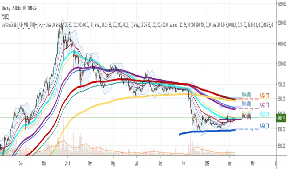
Multi SMA EMA WMA HMA BB (5x8 MAs Bollinger Bands) MAX MTF - RRBMulti SMA EMA WMA HMA 4x7 Moving Averages with Bollinger Bands MAX MTF by RagingRocketBull 2019
Version 1.0
All available MAX MTF versions are listed below (They are very similar and I don't want to publish them as separate indicators):
ver 1.0: 4x7 = 28 MTF MAs + 28 Levels + 3 BB = 59 < 64
ver 2.0: 5x6 = 30 MTF MAs + 30 Levels + 3 BB = 63 < 64
ver 3.0: 3x10 = 30 MTF MAs + 30 Levels + 3 BB = 63 < 64
ver 4.0: 5(4+1)x8 = 8 CurTF MAs + 32 MTF MAs + 20 Levels + 3 BB = 63 < 64
ver 5.0: 6(5+1)x6 = 6 CurTF MAs + 30 MTF MAs + 24 Levels + 3 BB = 63 < 64
ver 6.0: 4(3+1)x10 = 10 CurTF MAs + 30 MTF MAs + 20 Levels + 3 BB = 63 < 64
Fib numbers: 8, 13, 21, 34, 55, 89, 144, 233, 377
This indicator shows multiple MAs of any type SMA EMA WMA HMA etc with BB and MTF support, can show MAs as dynamically moving levels.
There are 4 MA groups + 1 BB group, a total of 4 TFs * 7 MAs = 28 MAs. You can assign any type/timeframe combo to a group, for example:
- EMAs 9,12,26,50,100,200,400 x H1, H4, D1, W1 (4 TFs x 7 MAs x 1 type)
- EMAs 8,13,21,30,34,50,55,89,100,144,200,233,377,400 x M15, H1 (2 TFs x 14 MAs x 1 type)
- D1 EMAs and SMAs 8,13,21,30,34,50,55,89,100,144,200,233,377,400 (1 TF x 14 MAs x 2 types)
- H1 WMAs 13,21,34,55,89,144,233; H4 HMAs 9,12,26,50,100,200,400; D1 EMAs 12,26,89,144,169,233,377; W1 SMAs 9,12,26,50,100,200,400 (4 TFs x 7 MAs x 4 types)
- +1 extra MA type/timeframe for BB
There are several versions: Simple, MTF, Pro MTF, Advanced MTF, MAX MTF and Ultimate MTF. This is the MAX MTF version. The Differences are listed below. All versions have BB
- Simple: you have 2 groups of MAs that can be assigned any type (5+5)
- MTF: +2 custom Timeframes for each group (2x5 MTF) +1 TF for BB, TF XY smoothing
- Pro MTF: 4 custom Timeframes for each group (4x3 MTF), 1 TF for BB, MA levels and show max bars back options
- Advanced MTF: +4 extra MAs/group (4x7 MTF), custom Ticker/Symbols, Timeframe <>= filter, Remove Duplicates Option
- MAX MTF: +2 subtypes/group, packed to the limit with max possible MAs/TFs: 4x7, 5x6, 3x10, 4(3+1)x10, 5(4+1)x8, 6(5+1)x6
- Ultimate MTF: +individual settings for each MA, custom Ticker/Symbols
MAX MTF version tests the limits of Pinescript trying to squeeze as many MAs/TFs as possible into a single indicator.
It's basically a maxed out Advanced version with subtypes allowing for mixed types within a group (i.e. both emas and smas in a single group/TF)
Pinescript has the following limits:
- max 40 security calls (6 calls are reserved for dupe checks and smoothing, 2 are used for BB, so only 32 calls are available)
- max 64 plot outputs (BB uses 3 outputs, so only 61 plot outputs are available)
- max 50000 (50kb) size of the compiled code
Based on those limits, you can only have the following MAs/TFs combos in a single script:
1. 4x7, 5x6, 3x10 - total number of MTF MAs must always be <= 32, and you can still have BB and Num Levels = total MAs, without any compromises
2. 5(4+1)x8, 6(5+1)x6, 4(3+1)x10 - you can use the Current Symbol/Timeframe as an extra (+1) fixed TF with the same number of MTF MAs
- you don't need to call security to display MAs on the Current Symbol/Timeframe, so the total number of MTF MAs remains the same and is still <= 32
- to fit that many MAs into the max 64 plot outputs limit you need to reduce the number of levels (not every MA Group will have corresponding levels)
Features:
- 4x7 = 28 MAs of any type
- 4x MTF groups with XY step line smoothing
- +1 extra TF/type for BB MAs
- 2 MA subtypes within each group/TF
- 4x7 = 28 MA levels with adjustable group offsets, indents and shift
- supports any existing type of MA: SMA, EMA, WMA, Hull Moving Average (HMA)
- custom tickers/symbols for each group
- show max bars back option
- show/hide both groups of MAs/levels/BB and individual MAs
- timeframe filter: show only MAs/Levels with TFs <>= Current TF
- hide MAs/Levels with duplicate TFs
- support for custom TFs that are not available in free accounts: 2D, 3D etc
- support for timeframes in H: H, 2H, 4H etc
Notes:
- Uses timeframe textbox instead of input resolution dropdown to allow for 240 120 and other custom TFs
- Uses symbol textbox instead of input symbol to avoid establishing multiple dummy security connections to the current ticker - otherwise empty symbols will prevent script from running
- Possible reasons for missing MAs on a chart:
- there may not be enough bars in history to start plotting it. For example, W1 EMA200 needs at least 200 bars on a weekly chart.
- for charts with low/fractional prices i.e. 0.00002 << 0.001 (default Y smoothing step) decrease Y smoothing as needed (set Y = 0.0000001) or disable it completely (set X,Y to 0,0)
- for charts with high price values i.e. 20000 >> 0.001 increase Y smoothing as needed (set Y = 10-20). Higher values exceeding MAs point density will cause it to disappear as there will be no points to plot. Different TFs may require diff adjustments
- TradingView Replay Mode UI and Pinescript security calls are limited to TFs >= D (D,2D,W,MN...) for free accounts
- attempting to plot any TF < D1 in Replay Mode will only result in straight lines, but all TFs will work properly in history and real-time modes. This is not a bug.
- Max Bars Back (num_bars) is limited to 5000 for free accounts (10000 for paid), will show error when exceeded. To plot on all available history set to 0 (default)
- Slow load/redraw times. This indicator becomes slower, its UI less responsive when:
- Pinescript Node.js graphics library is too slow and inefficient at plotting bars/objects in a browser window. Code optimization doesn't help much - the graphics engine is the main reason for general slowness.
- the chart has a long history (10000+ bars) in a browser's cache (you have scrolled back a couple of screens in a max zoom mode).
- Reload the page/Load a fresh chart and then apply the indicator or
- Switch to another Timeframe (old TF history will still remain in cache and that TF will be slow)
- in max possible zoom mode around 4500 bars can fit on 1 screen - this also slows down responsiveness. Reset Zoom level
- initial load and redraw times after a param change in UI also depend on TF. For example: D1/W1 - 2 sec, H1/H4 - 5-6 sec, M30 - 10 sec, M15/M5 - 4 sec, M1 - 5 sec. M30 usually has the longest history (up to 16000 bars) and W1 - the shortest (1000 bars).
- when indicator uses more MAs (plots) and timeframes it will redraw slower. Seems that up to 5 Timeframes is acceptable, but 6+ Timeframes can become very slow.
- show_last=last_bars plot limit doesn't affect load/redraw times, so it was removed from MA plot
- Max Bars Back (num_bars) default/custom set UI value doesn't seem to affect load/redraw times
- In max zoom mode all dynamic levels disappear (they behave like text)
- Dupe check includes symbol: symbol, tf, both subtypes - all must match for a duplicate group
- For the dupe check to work correctly a custom symbol must always include an exchange prefix. BB is not checked for dupes
Good Luck! Feel free to learn from/reuse the code to build your own indicators.
"北证50+股票+新浪财经"に関するスクリプトを検索

Multi SMA EMA WMA HMA BB (4x5 MAs Bollinger Bands) Adv MTF - RRBMulti SMA EMA WMA HMA 4x5 Moving Averages with Bollinger Bands Advanced MTF by RagingRocketBull 2019
Version 1.0
This indicator shows multiple MAs of any type SMA EMA WMA HMA etc with BB and MTF support, can show MAs as dynamically moving levels.
There are 4 MA groups + 1 BB group, a total of 4 TFs * 5 MAs = 20 MAs. You can assign any type/timeframe combo to a group, for example:
- EMAs 12,26,50,100,200 x H1, H4, D1, W1 (4 TFs x 5 MAs x 1 type)
- EMAs 8,10,13,21,30,50,55,100,200,400 x M15, H1 (2 TFs x 10 MAs x 1 type)
- D1 EMAs and SMAs 8,10,12,26,30,50,55,100,200,400 (1 TF x 10 MAs x 2 types)
- H1 WMAs 7,77,89,167,231; H4 HMAs 12,26,50,100,200; D1 EMAs 89,144,169,233,377; W1 SMAs 12,26,50,100,200 (4 TFs x 5 MAs x 4 types)
- +1 extra MA type/timeframe for BB
There are several versions: Simple, MTF, Pro MTF, Advanced MTF and Ultimate MTF. This is the Advanced MTF version. The Differences are listed below. All versions have BB
- Simple: you have 2 groups of MAs that can be assigned any type (5+5)
- MTF: +2 custom Timeframes for each group (2x5 MTF) +1 TF for BB, TF XY smoothing
- Pro MTF: 4 custom Timeframes for each group (4x3 MTF), 1 TF for BB, MA levels and show max bars back options
- Advanced MTF: +2 extra MAs/group (4x5 MTF), custom Ticker/Symbols, Timeframe <>= filter, Remove Duplicates Option
- Ultimate MTF: +individual settings for each MA, custom Ticker/Symbols
Features:
- 4x5 = 20 MAs of any type
- 4x MTF groups with XY step line smoothing
- +1 extra TF/type for BB MAs
- 4x5 = 20 MA levels with adjustable group offsets, indents and shift
- supports any existing type of MA: SMA, EMA, WMA, Hull Moving Average (HMA)
- custom tickers/symbols for each group - you can compare MAs of the same symbol across exchanges
- show max bars back option
- show/hide both groups of MAs/levels/BB and individual MAs
- timeframe filter: show only MAs/Levels with TFs <>= Current TF
- hide MAs/Levels with duplicate TFs
- support for custom TFs that are not available in free accounts: 2D, 3D etc
- support for timeframes in H: H, 2H, 4H etc
Notes:
- Uses timeframe textbox instead of input resolution dropdown to allow for 240 120 and other custom TFs
- Uses symbol textbox instead of input symbol to avoid establishing multiple dummy security connections to the current ticker - otherwise empty symbols will prevent script from running
- Possible reasons for missing MAs on a chart:
- there may not be enough bars in history to start plotting it. For example, W1 EMA200 needs at least 200 bars on a weekly chart.
- price << default Y smoothing step 5. For charts with low/fractional prices (i.e. 0.00002 << 5) adjust X Y smoothing as needed (set Y = 0.0000001) or disable it completely (set X,Y to 0,0)
- TradingView Replay Mode UI and Pinescript security calls are limited to TFs >= D (D,2D,W,MN...) for free accounts
- attempting to plot any TF < D1 in Replay Mode will only result in straight lines, but all TFs will work properly in history and real-time modes. This is not a bug.
- Max Bars Back (num_bars) is limited to 5000 for free accounts (10000 for paid), will show error when exceeded. To plot on all available history set to 0 (default)
- Slow load/redraw times. This indicator becomes slower, its UI less responsive when:
- Pinescript Node.js graphics library is too slow and inefficient at plotting bars/objects in a browser window. Code optimization doesn't help much - the graphics engine is the main reason for general slowness.
- the chart has a long history (10000+ bars) in a browser's cache (you have scrolled back a couple of screens in a max zoom mode).
- Reload the page/Load a fresh chart and then apply the indicator or
- Switch to another Timeframe (old TF history will still remain in cache and that TF will be slow)
- in max possible zoom mode around 4500 bars can fit on 1 screen - this also slows down responsiveness. Reset Zoom level
- initial load and redraw times after a param change in UI also depend on TF. For example:
D1/W1 - 2 sec, H1/H4 - 5-6 sec, M30 - 10 sec, M15/M5 - 4 sec, M1 - 5 sec.
M30 usually has the longest history (up to 16000 bars) and W1 - the shortest (1000 bars).
- when indicator uses more MAs (plots) and timeframes it will redraw slower. Seems that up to 5 Timeframes is acceptable, but 6+ Timeframes can become very slow.
- show_last=last_bars plot limit doesn't affect load/redraw times, so it was removed from MA plot
- Max Bars Back (num_bars) default/custom set UI value doesn't seem to affect load/redraw times
- In max zoom mode all dynamic levels disappear (they behave like text)
1. based on 3EmaBB, uses plot*, barssince and security functions
2. you can't set certain constants from input due to Pinescript limitations - change the code as needed, recompile and use as a private version
3. Levels = trackprice implementation
4. Show Max Bars Back = show_last implementation
5. swma has a fixed length = 4, alma and linreg have additional offset and smoothing params
6. Smoothing is applied by default for visual aesthetics on MTF. To use exact ma mtf values (lines with stair stepping) - disable it
Good Luck! You can explore, modify/reuse the code to build your own indicators.
BB Quick Fire5 Bollinger Bands in levels 50,2.0 | 50,2.5 |50,3.0 |50,3.5 |50,4.0
This is used to identify pullbakcs and future pitchfork's.

CM Stochastic POP Method 2-Jake Bernstein_V1Yesterday Jake Bernstein authorized me to post his updated results with the Stochastic Pop Trading System he developed many years ago.
You can take a look at the Original System with Updated Settings at
This indicator is a different set of rules Jake mentioned in the PDF he allowed me to post.
To view the PDF use this link:
dl.dropboxusercontent.com
Today we’re releasing the version described in the PDF that uses the StochK values of 55, 50, and 45. The rules are discussed in the PDF but here is a simple breakdown:
Enter Long when StochK is below 50 and Crosses Above 55
Exit Long on Cross Below 55
Enter Short when StochK is Above 50 and crosses Below 45
Exit Short on Cross Above 45
Two Important Items to understand about this method:
To code the rules Precisely we need a function that will be available when Strategy Capabilities are released on TradingView.
There is one of Jakes Profit Maximizing Strategies that needs to be integrated with this code…which again we need the Strategy based Function that will be coming soon.
To Compare this system to the Stochastic Pop Method 1 System shown yesterday at I used the same Symbol and dates for you to compare…but remember to give this Method 2 System a Fair Look/Evaluation…we need the Soon To Be Released…TradingView Strategy Capabilities.
BackTesting Results Example: EUR-USD Daily Chart Since 01/01/2005
Strategy 1 – Stochastic Pop Method 2 System:
Go Long When Stochasticis below 50 and Crosses Above 55. Go Short When Stochastic is above 50 and Crosses Below 45. Exit Long/Short When Stochastic has a Reverse Cross of Entry Value.
Results:
Total Trades = 151
Profit = 40,758 Pips
Win% = 37.1%
Profit Factor = 1.26
Avg Trade = 270 Pips Profit
***Most Consecutive Wins = 4 ... Most Consecutive Losses = 7
Strategy 2:
Rules - Proprietary Optimization Jake Will Teach. Only Added 1 Additional Exit Rule.
Results:
Total Trades = 151
Profit = 60.305 Pips
Win% = 37.1%
Profit Factor = 1.38
Avg Trade = 399 Pips Profit
***Most Consecutive Wins = 4 ... Most Consecutive Losses = 7
Indicator Includes:
-Ability to Color Candles (CheckBox In Inputs Tab)
Green = Long Trade
Blue = No Trade
Red = Short Trade
Jake Bernstein will be a contributor on TradingView when Backtesting/Strategies are released. Jake is one of the Top Trading System Developers in the world with 45+ years experience and he is going to teach TradingView.com’s community how to create Trading Systems and how to Optimize the correct way.
Link To PDF:
dl.dropboxusercontent.com
Link to Original Version of Indicator with Updated Settings.

MTF RSI Stacked + AI + Gradient MTF RSI Stacked + AI + Gradient
Quick-start guide & best-practice rules
What the indicator does
Multi-Time-Frame RSI in one pane
• 10 time-frames (1 m → 1 M) are stacked 100 points apart (0, 100, 200 … 900).
• Each RSI is plotted with a smooth red-yellow-green gradient:
– Red = RSI below 30 (oversold)
– Yellow = RSI near 50
– Green = RSI above 70 (overbought)
• Grey 30-70 bands are drawn for every TF so you can see extremities at a glance.
Built-in AI (KNN) signal
• On every close of the chosen AI-time-frame the script:
– Takes the last 14-period RSI + normalised ATR as “features”
– Compares them to the last N bars (default 1 000)
– Votes of the k = 5 closest neighbours → BUY / SELL / NEUTRAL
• Confidence % is shown in the badge (top-right).
• A thick vertical line (green/red) is printed once when the signal flips.
How to read it
• Gradient colour tells you instantly which TFs are overbought/obove sold.
• When all or most gradients are green → broad momentum up; look for shorts only on lower-TF pullbacks.
• When most are red → broad momentum down; favour longs only on lower-TF bounces.
• Use the AI signal as a confluence filter, not a stand-alone entry:
– If AI = BUY and 3+ higher-TF RSIs just crossed > 50 → consider long.
– If AI = SELL and 3+ higher-TF RSIs just crossed < 50 → consider short.
• Divergences: price makes a higher high but 1 h/4 h RSI (gradient) makes a lower high → possible reversal.
Settings you can tweak
AI timeframe – leave empty = same as chart, or pick a higher TF (e.g. “15” or “60”) to slow the signal down.
Training bars – 500-2 000 is the sweet spot; bigger = slower but more stable.
K neighbours – 3-7; lower = more signals, higher = smoother.
RSI length – 14 is standard; 9 gives earlier turns, 21 gives fewer false swings.
Practical trading workflow
Open the symbol on your execution TF (e.g. 5 m).
Set AI timeframe to 3-5× execution TF (e.g. 15 m or 30 m) so the signal survives market noise.
Wait for AI signal to align with gradient extremes on at least one higher TF.
Enter on the first gradient reversal inside the 30-70 band on the execution TF.
Place stop beyond the swing that caused the gradient flip; target next opposing 70/30 level on the same TF or trail with structure.
Colour cheat-sheet
Bright green → RSI ≥ 70 (overbought)
Bright red → RSI ≤ 30 (oversold)
Muted colours → RSI near 50 (neutral, momentum pause)
That’s it—one pane, ten time-frames, colour-coded extremes and an AI confluence layer.
Keep the chart clean, use price action for precise entries, and let the gradient tell you when the wind is at your back.

Kịch bản của tôi//@version=6
indicator(title="Relative Strength Index", shorttitle="Gấu Trọc RSI", format=format.price, precision=2, timeframe="", timeframe_gaps=true)
rsiLengthInput = input.int(14, minval=1, title="RSI Length", group="RSI Settings")
rsiSourceInput = input.source(close, "Source", group="RSI Settings")
calculateDivergence = input.bool(false, title="Calculate Divergence", group="RSI Settings", display = display.data_window, tooltip = "Calculating divergences is needed in order for divergence alerts to fire.")
change = ta.change(rsiSourceInput)
up = ta.rma(math.max(change, 0), rsiLengthInput)
down = ta.rma(-math.min(change, 0), rsiLengthInput)
rsi = down == 0 ? 100 : up == 0 ? 0 : 100 - (100 / (1 + up / down))
rsiPlot = plot(rsi, "RSI", color=#7E57C2)
rsiUpperBand1 = hline(98, "RSI Upper Band1", color=#787B86)
rsiUpperBand = hline(70, "RSI Upper Band", color=#787B86)
midline = hline(50, "RSI Middle Band", color=color.new(#787B86, 50))
rsiLowerBand = hline(30, "RSI Lower Band", color=#787B86)
rsiLowerBand2 = hline(14, "RSI Lower Band2", color=#787B86)
fill(rsiUpperBand, rsiLowerBand, color=color.rgb(126, 87, 194, 90), title="RSI Background Fill")
midLinePlot = plot(50, color = na, editable = false, display = display.none)
fill(rsiPlot, midLinePlot, 100, 70, top_color = color.new(color.green, 0), bottom_color = color.new(color.green, 100), title = "Overbought Gradient Fill")
fill(rsiPlot, midLinePlot, 30, 0, top_color = color.new(color.red, 100), bottom_color = color.new(color.red, 0), title = "Oversold Gradient Fill")
// Smoothing MA inputs
GRP = "Smoothing"
TT_BB = "Only applies when 'SMA + Bollinger Bands' is selected. Determines the distance between the SMA and the bands."
maTypeInput = input.string("SMA", "Type", options = , group = GRP, display = display.data_window)
var isBB = maTypeInput == "SMA + Bollinger Bands"
maLengthInput = input.int(14, "Length", group = GRP, display = display.data_window, active = maTypeInput != "None")
bbMultInput = input.float(2.0, "BB StdDev", minval = 0.001, maxval = 50, step = 0.5, tooltip = TT_BB, group = GRP, display = display.data_window, active = isBB)
var enableMA = maTypeInput != "None"
// Smoothing MA Calculation
ma(source, length, MAtype) =>
switch MAtype
"SMA" => ta.sma(source, length)
"SMA + Bollinger Bands" => ta.sma(source, length)
"EMA" => ta.ema(source, length)
"SMMA (RMA)" => ta.rma(source, length)
"WMA" => ta.wma(source, length)
"VWMA" => ta.vwma(source, length)
// Smoothing MA plots
smoothingMA = enableMA ? ma(rsi, maLengthInput, maTypeInput) : na
smoothingStDev = isBB ? ta.stdev(rsi, maLengthInput) * bbMultInput : na
plot(smoothingMA, "RSI-based MA", color=color.yellow, display = enableMA ? display.all : display.none, editable = enableMA)
bbUpperBand = plot(smoothingMA + smoothingStDev, title = "Upper Bollinger Band", color=color.green, display = isBB ? display.all : display.none, editable = isBB)
bbLowerBand = plot(smoothingMA - smoothingStDev, title = "Lower Bollinger Band", color=color.green, display = isBB ? display.all : display.none, editable = isBB)
fill(bbUpperBand, bbLowerBand, color= isBB ? color.new(color.green, 90) : na, title="Bollinger Bands Background Fill", display = isBB ? display.all : display.none, editable = isBB)
// Divergence
lookbackRight = 5
lookbackLeft = 5
rangeUpper = 60
rangeLower = 5
bearColor = color.red
bullColor = color.green
textColor = color.white
noneColor = color.new(color.white, 100)
_inRange(bool cond) =>
bars = ta.barssince(cond)
rangeLower <= bars and bars <= rangeUpper
plFound = false
phFound = false
bullCond = false
bearCond = false
rsiLBR = rsi
if calculateDivergence
//------------------------------------------------------------------------------
// Regular Bullish
// rsi: Higher Low
plFound := not na(ta.pivotlow(rsi, lookbackLeft, lookbackRight))
rsiHL = rsiLBR > ta.valuewhen(plFound, rsiLBR, 1) and _inRange(plFound )
// Price: Lower Low
lowLBR = low
priceLL = lowLBR < ta.valuewhen(plFound, lowLBR, 1)
bullCond := priceLL and rsiHL and plFound
//------------------------------------------------------------------------------
// Regular Bearish
// rsi: Lower High
phFound := not na(ta.pivothigh(rsi, lookbackLeft, lookbackRight))
rsiLH = rsiLBR < ta.valuewhen(phFound, rsiLBR, 1) and _inRange(phFound )
// Price: Higher High
highLBR = high
priceHH = highLBR > ta.valuewhen(phFound, highLBR, 1)
bearCond := priceHH and rsiLH and phFound
plot(
plFound ? rsiLBR : na,
offset = -lookbackRight,
title = "Regular Bullish",
linewidth = 2,
color = (bullCond ? bullColor : noneColor),
display = display.pane,
editable = calculateDivergence)
plotshape(
bullCond ? rsiLBR : na,
offset = -lookbackRight,
title = "Regular Bullish Label",
text = " Bull ",
style = shape.labelup,
location = location.absolute,
color = bullColor,
textcolor = textColor,
display = display.pane,
editable = calculateDivergence)
plot(
phFound ? rsiLBR : na,
offset = -lookbackRight,
title = "Regular Bearish",
linewidth = 2,
color = (bearCond ? bearColor : noneColor),
display = display.pane,
editable = calculateDivergence)
plotshape(
bearCond ? rsiLBR : na,
offset = -lookbackRight,
title = "Regular Bearish Label",
text = " Bear ",
style = shape.labeldown,
location = location.absolute,
color = bearColor,
textcolor = textColor,
display = display.pane,
editable = calculateDivergence)
alertcondition(bullCond, title='Regular Bullish Divergence', message="Found a new Regular Bullish Divergence, `Pivot Lookback Right` number of bars to the left of the current bar.")
alertcondition(bearCond, title='Regular Bearish Divergence', message='Found a new Regular Bearish Divergence, `Pivot Lookback Right` number of bars to the left of the current bar.')
Daily Oversold Swing ScreenerThat script is a **Pine Script Indicator** designed to identify potential **swing trade entry points** on a daily timeframe by looking for stocks that are **oversold** but still in a **healthy long-term uptrend**.
It screens for a high-probability reversal setup by combining four specific technical conditions.
Here is a detailed breakdown of the script's purpose and logic:
---
## 📝 Script Description: Daily Oversold Swing Screener
This Pine Script indicator serves as a **momentum and trend confirmation tool** for active traders seeking short-to-intermediate-term long entries. It uses data calculated on the **Daily** timeframe to generate signals, regardless of the chart resolution you are currently viewing.
The indicator is designed to filter out stocks that are in a strong downtrend ("falling knives") and only signal pullbacks within an established uptrend, which significantly increases the probability of a successful swing trade bounce.
### 🔑 Key Conditions for a Signal:
The indicator generates a buy signal when **all four** of the following conditions are met on the Daily timeframe:
#### 1. Oversold Momentum
* **Condition:** `rsiD < rsiOS` (Daily RSI is below the oversold level, typically **30**).
* **Purpose:** Confirms that the selling pressure has been extreme and the stock is temporarily out of favor, setting up a potential bounce.
#### 2. Momentum Turning Up
* **Condition:** `rsiD > rsiPrev` (Current Daily RSI value is greater than the previous day's Daily RSI value).
* **Purpose:** This is the most crucial filter. It confirms that the momentum has **just started to shift upward**, indicating that the low may be in and the stock is turning away from the oversold region.
#### 3. Established Uptrend (No Falling Knives)
* **Condition:** `sma50 > sma200 and closeD > sma50` (50-day SMA is above the 200-day SMA, AND the current daily close is above the 50-day SMA).
* **Purpose:** This is a **long-term trend filter**. It ensures that the current oversold condition is just a **pullback** within a larger, structurally bullish market (50 > 200), and that the price is still holding above the short-term trend line (Close > 50 SMA). This effectively screens out weak stocks in continuous downtrends.
#### 4. Price at Support (Bollinger Bands)
* **Condition:** `closeD <= lowerBB` (Daily Close is less than or equal to the lower Bollinger Band).
* **Purpose:** Provides a secondary measure of extreme price deviation. When the price touches or breaches the lower band, it suggests a significant move away from the mean (basis), often signaling strong statistical support where price is likely to revert.
### 📌 Summary of Signal
The final signal (`signal`) is triggered only when the market is confirmed to be **in a healthy long-term trend (Condition 3)**, the price is at an **extreme support level (Condition 4)**, the momentum is **oversold (Condition 1)**, and most importantly, the **momentum has begun to reverse (Condition 2)**.

Dynamic SMA Trend System [Multi-Stage Risk Engine]Description:
This script implements a robust Trend Following strategy based on a multiple Simple Moving Average (SMA) crossover logic (25, 50, 100, 200). What sets this strategy apart is its advanced "4-Stage Risk Engine" and a smart "High-Water Mark" Re-Entry system, designed to protect profits during parabolic moves while filtering out chop during sideways markets.
How it works:
The strategy operates on three core pillars: Trend Identification, Dynamic Risk Management, and Momentum Re-Entry.
1. Entry Logic (Trend Identification) The script looks for crossovers at different trend stages to capture early reversals as well as established trends:
Short-Term: SMA 25 crosses over SMA 50.
Mid-Term: SMA 50 crosses over SMA 100.
Macro-Trend: SMA 100 crosses over SMA 200.
2. The 4-Stage Risk Engine (Dynamic Stop Loss) Instead of a static Stop Loss, this strategy uses a progressive system that adapts as the price increases:
Stage 1 (Protection): Starts with a fixed Stop Loss (default -10%) to give the trade room to breathe.
Stage 2 (Break-Even): Once the price rises by 12%, the Stop is moved to trailing mode (10% distance), effectively securing a near break-even state.
Stage 3 (Profit Locking): At 25% profit, the trailing stop tightens to 8% to lock in gains.
Stage 4 (Parabolic Mode): At 40% profit, the trailing stop tightens further to 5% to capture the peak of parabolic moves.
3. Dual Exit Mechanism The strategy exits a position if EITHER of the following happens:
Stop Loss Hit: Price falls below the dynamic red line (Risk Engine).
Dead Cross: The trend structure breaks (e.g., SMA 25 crosses under SMA 50), signaling a momentum loss even if the Stop Loss wasn't hit.
4. "High-Water Mark" Re-Entry To avoid "whipsaws" in choppy markets, the script does not re-enter immediately after a stop-out.
It marks the highest price of the previous trade (Green Dotted Line).
A Re-Entry only occurs if the price breaks above this previous high (showing renewed strength) AND the long-term trend is bullish (Price > SMA 200).
Visuals:
SMAs: 25 (Yellow), 50 (Orange), 100 (Blue), 200 (White).
Red Line: Visualizes the dynamic Stop Loss level.
Green Dots: Visualizes the target price needed for a valid re-entry.
Settings: All parameters (SMA lengths, Stop Loss percentages, Staging triggers) are fully customizable in the settings menu to fit different assets (Crypto, Stocks, Forex) and timeframes.

Every Hour 1st/Last FVG vTDL OVERVIEW - Shoutout to Micheal J. Huddleston aka ICT
This indicator identifies the first Fair Value Gap (FVG) that forms within each trading hour, providing traders with potential entry zones, reversal points, and unmitigated gap targets. Based on the concept that the first presented FVG of each hour represents a significant price delivery array where institutional order flow occurred.
The indicator detects FVGs on a lower timeframe (1-minute default) and displays them as boxes on your chart, tracking which gaps get filled and which remain open as potential draw-on-liquidity targets.
WHAT IS A FAIR VALUE GAP
A Fair Value Gap is a 3-candle price pattern representing an imbalance between buyers and sellers:
Bullish FVG: Forms when candle 3's low is above candle 1's high, leaving a gap
Bearish FVG: Forms when candle 3's high is below candle 1's low, leaving a gap
These gaps often act as magnets for price, which tends to return and "fill" the imbalance before continuing. They function as dynamic support and resistance zones.
KEY FEATURES
Detection Types
FVG: Standard fair value gap detection with volume imbalance expansion
Suspension FVG Blocks: Requires outside prints on both sides for more refined signals
Hourly Display Modes
First Only: Shows whichever FVG appears first each hour (bullish or bearish)
Show Both: Shows first bullish AND first bearish FVG independently each hour
Last FVG Tracking
Optionally display the last FVG of each hour
Useful for comparing how the hour developed
Can extend into the next hour for continued tracking
Breakaway Gap Detection
Gaps not traded into during their formation hour extend forward
Extended gaps display labels showing formation time and date
These unmitigated gaps become price targets and reversal zones
Gap Fill Modes
Touch Box: Marks filled when price enters the gap
Touch Midpoint: Marks filled when price reaches the 50 percent level
Fill Completely: Marks filled when price fills the entire gap with visual progress
HOW TO USE
Entry Points
The first FVG of each hour provides potential entry zones based on price reaction:
When price returns to an FVG and shows rejection, enter in the direction of rejection
The gap zone represents where institutional orders likely reside
Use the boundaries of the gap for stop loss placement
A clean rejection of the zone confirms it as valid support or resistance
Reversal Points
Unmitigated gaps that extend beyond their formation hour are high-probability reaction zones:
Extended boxes with labels indicate unfilled gaps
When price finally reaches these zones, expect a reaction
The longer a gap remains unfilled, the stronger the expected response
These zones act as magnets drawing price back to them
Price Targets
Use unmitigated gaps as draw-on-liquidity targets:
Look for extended boxes above or below current price
Price tends to seek out and fill imbalances
The midpoint line often serves as a minimum target
Multiple unfilled gaps in one direction suggest strong momentum potential
FRAMING DIRECTIONAL BIAS
The first presented FVG of each hour acts as a support or resistance zone. The direction of the FVG itself does not determine bias - it is how price reacts to that FVG that reveals the true market intention.
Reading Price Reaction
Price respects a bullish FVG as support and bounces higher = bullish bias confirmed
Price respects a bearish FVG as resistance and rejects lower = bearish bias confirmed
Price fails to hold a bullish FVG and breaks through = potential inversion, look for shorts
Price fails to hold a bearish FVG and breaks through = potential inversion, look for longs
Inversion Fair Value Gaps (IFVG)
When price trades through an FVG and closes beyond it, that gap can invert its role:
A bullish FVG that fails becomes resistance - use it as a short entry zone
A bearish FVG that fails becomes support - use it as a long entry zone
The inversion signals a shift in control from one side to the other
Watch for price to retest the inverted gap before continuing
Support and Resistance Framework
Think of each hourly first FVG as a key level:
Price above the FVG: the gap acts as potential support
Price below the FVG: the gap acts as potential resistance
Watch how price behaves when it returns to the gap zone
A clean rejection confirms the level; a break through signals inversion
SHORT-TERM SCALPING APPLICATION
These FVGs provide scalping opportunities each hour:
Identify the first FVG of the hour as your key level
Wait for price to trade away from it and return
Observe the reaction at the gap zone
Enter in the direction of the reaction with tight risk
Target the next FVG, midpoint, or nearby liquidity
Trade Management
Use the opposite side of the FVG box as your stop loss zone
The midpoint of the gap often provides first target or decision point
Scale out at nearby unmitigated gaps or key levels
If the gap inverts, flip your bias and look for entries in the new direction
MULTI-HOUR CONTEXT
If price consistently respects FVGs as support across hours = uptrend context
If price consistently respects FVGs as resistance across hours = downtrend context
If FVGs keep inverting = choppy or transitional market
Use higher timeframe direction to filter which reactions to trade
Compare first and last FVG of each hour to see how momentum developed
SESSION FILTERING
The indicator automatically excludes unreliable periods:
4 PM to 5 PM New York time (market close hours 16-17)
Weekend closed periods (Saturday and Sunday before 6 PM)
All timestamps use New York timezone for consistency with futures market hours.
SETTINGS GUIDE
Detection Settings
Detection Type: Choose between standard FVG or Suspension FVG Blocks
Lower Timeframe: 15 seconds, 1 minute, or 5 minutes for gap detection
Min FVG Size: Minimum gap size in ticks to filter noise
Display Settings
Hourly Display Mode: First Only shows one gap per hour; Show Both shows first bull and bear
Show First FVG: Toggle visibility of first FVG boxes
Show Last FVG: Toggle visibility of last FVG boxes
Show Midpoint Lines: Display the 50 percent level of each gap
Show Unfilled Breakaway Gaps: Extend boxes until price fills them
Show Only Today: Reduce clutter by hiding older hourly boxes
Gap Fill Detection Mode
Touch Box: Gap marked filled when price enters the zone
Touch Midpoint: Gap marked filled when price reaches 50 percent level
Fill Completely: Gap marked filled only when fully closed, shows visual fill progress
Recommended Settings by Style
Scalping: 1 minute LTF, 4 tick minimum, Show Both mode, Touch Box fill
Day Trading: 1 minute LTF, 4-8 tick minimum, First Only mode, Touch Midpoint fill
Swing Context: 5 minute LTF, Show Unfilled Gaps enabled, Fill Completely mode
COLOR CODING
Blue boxes: First bullish FVG of the hour
Red boxes: First bearish FVG of the hour
Green boxes: Last bullish FVG of the hour
Orange boxes: Last bearish FVG of the hour
Black midpoint lines: 50 percent level of each gap
Filled portion overlay: Shows visual progress in Fill Completely mode
All colors are fully customizable in the settings menu.
PRACTICAL TIPS
The first FVG of each hour is a hidden PD array - treat it as a significant level
Not every gap produces a tradeable reaction - wait for confirmation
Gaps that remain unfilled for multiple hours carry more weight
Use the Show Both mode to see both bullish and bearish opportunities each hour
When multiple gaps cluster in one zone, that area becomes even more significant
Inversions are powerful signals - a failed level often leads to acceleration
NOTES
Works on any instrument and timeframe
Best used on intraday charts (1 minute to 15 minute) viewing 1 minute LTF gaps
Combine with higher timeframe analysis for confluence
These are probability zones, not guarantees - always use proper risk management
The indicator handles HTF to LTF data fetching automatically

Gap-Up Momentum Screener (S.S)
ENGLISH-VERSION
1) TradingView Gap Screener (for US stocks)
➤ Conditions
Gap-Up ≥ +3% (large gaps indicate institutional pressure)
Pre-market volume ≥ 150% of the 20-day average
RS line > 50
Price > 50 SMA
Market cap ≥ 1 billion USD
No penny stocks
2) Minervini Gap-Entry Strategy (Swing Trading)
This is a variant specifically optimized for gaps + momentum.
A) Setup Criteria
The stock must meet the following conditions:
Gap-Up ≥ +3%
First retracement ≤ 30% of the gap
High relative strength (RS line rising)
Volume on the gap day > 2× average
Price above 20 EMA, 50 SMA, 150 SMA, 200 SMA
No immediate resistance within 2–5%
B) Entry Setups
Entry 1: First Pullback Entry (FPE)
Wait for the first 1–3 day consolidation.
Entry → Breakout of the small range.
Stop → Below the low of the pullback.
Rule: No entry on the gap day itself.
Entry 2: High Tight Flag above the Gap
Stock rises > 10% after the gap
Then forms a 3–8 day sideways phase
Entry → Break above the flag’s high
Stop → Below the flag base
Entry 3: ORB Entry (Opening Range Breakout, 30 minutes)
Very effective for strong gaps.
Wait 30 minutes after the market opens
Entry → Break above the high of these first 30 minutes
Stop → Below the 30-minute low
C) Stop Levels
For FPE: 4–8%
For ORB: 1–2 × ATR(14)
For flags: 3–5%
D) Add Rules
Only if the stock continues showing strong volume:
Add on every new 3–5 day high
Add only above half-range levels
Maximum 3 adds
3) Early-Warning Module (Setup forming but not ready for entry)
This module marks stocks that are forming a setup but are not yet buyable.
➤ Criteria
Gap-Up ≥ 3%
Strong volume
Stock pulls back and consolidates (1–5 bars)
BUT no breakout yet
4) Exact Entry Checklist (Minervini-style, optimized for gaps)
Checklist before entry:
Gap ≥ +3%
20 EMA rising
Volume > 2× average
RS line rising
Price > 50 SMA
Pullback not deeper than 30% of the gap
3+ green signals from the Early-Warning diamonds
If all 7 are fulfilled → green light.
5) How to apply the strategy in daily practice
Morning (08:00–09:00)
Check the screener
Build your watchlist
Identify gaps
US Market Open (15:30)
Monitor the Early-Warning module
Sort gap momentum opportunities
16:00–17:00
Enter: First Pullback / ORB / Flag
Set stops
Determine position size based on risk
After 20:00
Check volume strength
If momentum fades → no more adds

Extended SOPR Indicator — SSOPR Tops (A/B toggle)Extended SOPR Indicator — SSOPR Tops and Lows (A/B toggle)
Observation-only. Data: Glassnode SOPR.
Overview
This indicator extends the classical SOPR (Spent Output Profit Ratio) to improve readability and reduce noise on charts. SOPR measures whether coins moved on-chain were spent at a profit or at a loss. In brief: SOPR > 1 → spending at profit; SOPR < 1 → spending at loss. SSOPR (from "Smoothed SOPR") applies optional log transform (centers baseline at 0), smoothing (standard or adaptive), and adds structured signals: Z‑score lows (capitulation), buy zones , and top detection after prolonged elevation.
Why extend SOPR? (SSOPR vs classical SOPR)
• Noise reduction: Raw daily SOPR can whipsaw around its baseline. SSOPR uses smoothing and (optionally) adaptive smoothing so regimes are visible without overfitting.
• Better readability: The log transform shifts the break-even line to 0, making “profit territory” (above 0) and “loss territory” (below 0) visually intuitive on oscillators.
• Actionable context: Z‑score highlights extreme lows (capitulation risk), a simple buy-zone threshold marks potential accumulation, and a structured top pattern (with a time factor) helps frame distribution phases after sustained elevation.
What the script plots
• Smoothed SOPR (SSOPR): An orange line representing the smoothed SOPR (with optional log transform and optional adaptive smoothing).
• Top markers: A red triangle appears once at the onset of a confirmed top pattern.
• Background shading:
– Soft green: Buy zone when SSOPR falls below the “Buy Threshold.” (+ Z‑score capitulation zones (extreme lows)).
– Soft red: Top‑zone shading when the top criteria are met but before the single triangle fires.
Inputs & parameters
• Smoothing Length (default 14): Base window for smoothing SSOPR. Higher values = smoother, slower response.
• Apply Log Transform (default ON): Uses log(SOPR) so the baseline is 0 (log(1)=0). Above 0 → net profit regime; below 0 → net loss regime.
• Adaptive Smoothing (default OFF): Expands smoothing length as volatility rises using a standard deviation proxy; reduces whipsaws while preserving structure.
• Z‑score Threshold for Lows (default −2.5): Highlights capitulation zones when SSOPR deviates far below its rolling mean.
• SSOPR Buy Threshold (default −0.02): Simple rule-of-thumb level for potential accumulation context when below (log scale).
• SSOPR Top Threshold (default +0.005): Minimum elevation required for “profit territory” when assessing tops (log scale).
• Min Bars Above Threshold Before Top (default 50): Ensures prolonged elevation before calling a top.
• Lookback for Peak Detection (default 50): Window used to locate the recent high.
• Drop % from Peak to Confirm Top (default 5%): Confirms the start of distribution from a local high.
• Highlight Background : Toggles shaded zones.
Top detection (indicator-only)
A top fires when ALL of the following are true:
SSOPR spent at least Min Bars Above Threshold above the Top Threshold (sustained elevation).
The rising phase test passes (Option A or B; see below).
A drop from the local peak exceeds Drop % within the Lookback window.
The peak occurred in profit territory (SSOPR > Top Threshold).
To avoid repeated signals during the decline, the script emits the triangle once, at onset.
Rising‑phase switch: Option A vs Option B
• Option A — Up‑step ratio : Over the last A: Bars for Rising Check (default 50), it requires that at least A: Required Up‑Step Ratio (default 60%) of bars were rising (each bar compared to the previous). This favors gradual, persistent advances and filters out “choppy” lifts.
• Option B — Net slope : Compares current SSOPR to its value B: Bars Back for Net Slope ago (default 50). If higher, the series is considered rising. This is simpler and reacts faster in volatile phases but can admit brief pseudo‑trends.
Guidance : Prefer A for conservative confirmation in slow, persistent cycles; use B when trend moves are strong and you need timely detection.
Interpretation guide
• Regimes (log view): Above 0 → spending at profit; below 0 → spending at loss.
• Capitulation lows: When Z‑score < threshold, conditions often reflect forced/liquidity‑driven spending. Treat as context, not signals.
• Buy zone: SSOPR < Buy Threshold flags potential accumulation conditions (combine with price structure).
• Tops: After prolonged elevation, a confirmed top often coincides with profit‑taking/distribution phases.
Recommended timeframes
• Daily : Code optimized for daily timeframe.
Method summary
• SSOPR source: GLASSNODE:BTC_SOPR (via request.security ).
• Optional log transform: sopr → log(sopr) to normalize around 0.
• Smoothing: SMA over Smoothing Length , optionally adaptive using local volatility (std dev).
• Z‑score: (SSOPR − mean) / std dev, highlighting extreme lows.
• Top: Requires long elevation above Top Threshold , rising‑phase (A/B), and a subsequent drop > Drop % from recent high.
Limitations & notes
• SOPR reflects on‑chain movements; some activity occurs off‑chain (exchanges, internal transfers). Not all moves imply sale; aggregation makes it a usable proxy for profit/loss realization.
• Higher smoothing reduces noise but delays signals; adaptive smoothing can help but is still a trade‑off.
• Treat thresholds as context markers. They are not entry/exit signals by themselves.
• Use with price structure, volume, and other on‑chain indicators (e.g., realized price bands, dormancy/CDD) for confluence.
How to use (examples)
• Advance holding above 0 (log view): Retests of 0 from above that hold—while SSOPR remains elevated—often mark absorption; look for Top conditions only after sustained elevation and a confirmed drop from peak.
• Downtrend below 0: Rejections near 0 can align with continued loss realization; extreme Z‑score lows suggest capitulation risk—context for accumulation, not a blind buy.
Recommended settings
• Weekly: Log ON, Smoothing Length 14–30, Adaptive ON, Buy Threshold −0.02, Top Threshold +0.005, Rising Method A, Min Bars 50.
• Daily: Log ON, Smoothing Length 14–20, Adaptive OFF or ON (depending on noise), Rising Method B for timely slope checks.
Credits & references
• SOPR metric: Renato Shirakashi; documentation: Glassnode , CryptoQuant , overview: Bitbo .
Disclaimer
This script is for research/education on market behavior. It is not financial advice. Indicators provide context; decisions remain your responsibility.
Tags
bitcoin, btc, on‑chain, sopr, ssopr, glassnode, oscillator, regime, distribution, capitulation

RSI adaptive zones [AdaptiveRSI]This script introduces a unified mathematical framework that auto-scales oversold/overbought and support/resistance zones for any period length. It also adds true RSI candles for spotting intrabar signals.
Built on the Logit RSI foundation, this indicator converts RSI into a statistically normalized space, allowing all RSI lengths to share the same mathematical footing.
What was once based on experience and observation is now grounded in math.
✦ ✦ ✦ ✦ ✦
💡 Example Use Cases
RSI(14): Classic overbought/oversold signals + divergence
Support in an uptrend using RSI(14)
Range breakouts using RSI(21)
Short-term pullbacks using RSI(5)
✦ ✦ ✦ ✦ ✦
THE PAST: RSI Interpretation Required Multiple Rulebooks
Over decades, RSI practitioners discovered that RSI behaves differently depending on trend and lookback length:
• In uptrends, RSI tends to hold higher support zones (40–50)
• In downtrends, RSI tends to resist below 50–60
• Short RSIs (e.g., RSI(2)) require far more extreme threshold values
• Longer RSIs cluster near the center and rarely reach 70/30
These observations were correct — but lacked a unifying mathematical explanation.
✦ ✦ ✦ ✦ ✦
THE PRESENT: One Framework Handles RSI(2) to RSI(200)
Instead of using fixed thresholds (70/30, 90/10, etc.), this indicator maps RSI into a normalized statistical space using:
• The Logit transformation to remove 0–100 scale distortion
• A universal scaling based on 2/√(n−1) scaling factor to equalize distribution shapes
As a result, RSI values become directly comparable across all lookback periods.
✦ ✦ ✦ ✦ ✦
💡 How the Adaptive Zones Are Calculated
The adaptive framework defines RSI zones as statistical regimes derived from the Logit-transformed RSI .
Each boundary corresponds to a standard deviation (σ) threshold, scaled by 2/√(n−1), making RSI distributions comparable across periods.
This structure was inspired by Nassim Nicholas Taleb’s body–shoulders–tails regime model:
Body (±0.66σ) — consolidation / equilibrium
Shoulders (±1σ to ±2.14σ) — trending region
Tails (outside of ±2.14σ) — rare, high-volatility behavior
Transitions between these regimes are defined by the derivatives of the position (CDF) function :
• ±1σ → shift from consolidation to trend
• ±√3σ → shift from trend to exhaustion
Adaptive Zone Summary
Consolidation: −0.66σ to +0.66σ
Support/Resistance: ±0.66σ to ±1σ
Uptrend/Downtrend: ±1σ to ±√3σ
Overbought/Oversold: ±√3σ to ±2.14σ
Tails: outside of ±2.14σ
✦ ✦ ✦ ✦ ✦
📌 Inverse Transformation: From σ-Space Back to RSI
A final step is required to return these statistically normalized boundaries back into the familiar 0–100 RSI scale. Because the Logit transform maps RSI into an unbounded real-number domain, the inverse operation uses the hyperbolic tangent function to compress σ-space back into the bounded RSI range.
RSI(n) = 50 + 50 · tanh(z / √(n − 1))
The result is a smooth, mathematically consistent conversion where the same statistical thresholds maintain identical meaning across all RSI lengths, while still expressing themselves as intuitive RSI values traders already understand.
✦ ✦ ✦ ✦ ✦
Key Features
Mathematically derived adaptive zones for any RSI period
Support/resistance zone identification for trend-aligned reversals
Optional OHLC RSI bars/candles for intrabar zone interactions
Fully customizable zone visibility and colors
Statistically consistent interpretation across all markets and timeframes
Inputs
RSI Length — core parameter controlling zone scaling
RSI Display : Line / Bar / Candle visualization modes
✦ ✦ ✦ ✦ ✦
💡 How to Use
This indicator is a framework , not a binary signal generator.
Start by defining the question you want answered, e.g.:
• Where is the breakout?
• Is price overextended or still trending?
• Is the correction ending, or is trend reversing?
Then:
Choose the RSI length that matches your timeframe
Observe which adaptive zone price is interacting with
Interpret market behavior accordingly
Example: Long-Term Trend Assesment using RSI(200)
A trader may ask: "Is this a long term top?"
Unlikely, because RSI(200) holds above Resistance zone , therefore the trend remains strong.
✦ ✦ ✦ ✦ ✦
👉 Practical tip:
If you used to overlay weekly RSI(14) on a daily chart (getting a line that waits 5 sessions to recalculate), you can now read the same long-horizon state continuously : set RSI(70) on the daily chart (~14 weeks × 5 days/week = 70 days) and let the adaptive zones update every bar .
Note: It won’t be numerically identical to the weekly RSI due to lookback period used, but it tracks the same regime on a standardized scale with bar-by-bar updates.
✦ ✦ ✦ ✦ ✦
Note: This framework describes statistical structure, not prediction. Use as part of a complete trading approach. Past behavior does not guarantee future outcomes.
framework ≠ guaranteed signal
---
Attribution & License
This indicator incorporates:
• Logit transformation of RSI
• Variance scaling using 2/√(n−1)
• Zone placement derived from Taleb’s body–shoulders–tails regime model and CDF derivatives
• Inverse TANH(z) transform for mapping z-scores back into bounded RSI space
Released under CC BY-NC-SA 4.0 — free for non-commercial use with credit.
© AdaptiveRSI
GRA v5 SNIPER# GRA v5 SNIPER - Documentation & Cheatsheet
## 🎯 Get Rich Aggressively v5 - SNIPER Edition
**Precision Futures Scalping | NQ • ES • YM • GC • BTC**
> **Philosophy:** *Quality over quantity. One sniper shot beats ten spray-and-pray attempts.*
---
## ⚡ QUICK CHEATSHEET
```
┌─────────────────────────────────────────────────────────────────────────────┐
│ GRA v5 SNIPER - QUICK REFERENCE │
├─────────────────────────────────────────────────────────────────────────────┤
│ │
│ 🎯 SIGNAL REQUIREMENTS (ALL MUST BE TRUE): │
│ ═══════════════════════════════════════════ │
│ ✓ Tier → B minimum (20+ pts NQ) │
│ ✓ Volume → 1.5x+ average │
│ ✓ Delta → 60%+ dominance (buyers OR sellers) │
│ ✓ Body → 70%+ of candle range │
│ ✓ Range → 1.3x+ average candle size │
│ ✓ Wicks → Small opposite wick (<50% of body) │
│ ✓ CVD → Trending with signal direction │
│ ✓ Session → London (3-5am ET) OR NY (9:30-11:30am ET) │
│ │
├─────────────────────────────────────────────────────────────────────────────┤
│ │
│ 📊 TIER ACTIONS: │
│ ════════════════ │
│ S-TIER (100+ pts) → 🥇 HOLD position, ride the wave │
│ A-TIER (50-99 pts) → 🥈 SWING for 2-3 minutes │
│ B-TIER (20-49 pts) → 🥉 SCALP quick, 30-60 seconds │
│ │
├─────────────────────────────────────────────────────────────────────────────┤
│ │
│ 🚨 ENTRY CHECKLIST: │
│ ═══════════════════ │
│ □ Signal appears (S🎯, A🎯, or B🎯) │
│ □ Table shows: Vol GREEN, Delta colored, Body GREEN │
│ □ CVD arrow matches direction (▲ for long, ▼ for short) │
│ □ Session active (LDN! or NY! in yellow) │
│ □ Enter at close of signal candle │
│ │
├─────────────────────────────────────────────────────────────────────────────┤
│ │
│ ⛔ DO NOT TRADE WHEN: │
│ ════════════════════ │
│ ✗ Session shows "---" (outside key hours) │
│ ✗ Vol shows RED (below 1.5x) │
│ ✗ Body shows RED (weak candle structure) │
│ ✗ Delta below 60% (no clear dominance) │
│ ✗ Multiple conflicting signals │
│ │
├─────────────────────────────────────────────────────────────────────────────┤
│ │
│ 📈 INSTRUMENT SETTINGS: │
│ ════════════════════════ │
│ NQ/ES (1-3 min): S=100, A=50, B=20 pts │
│ YM (1-5 min): S=100, A=50, B=25 pts │
│ GC (5-15 min): S=15, A=8, B=4 pts │
│ BTC (1-15 min): S=500, A=250, B=100 pts │
│ │
└─────────────────────────────────────────────────────────────────────────────┘
```
---
## 📋 DETAILED DOCUMENTATION
### What Makes SNIPER Different?
The SNIPER edition eliminates 80%+ of signals compared to standard GRA. Every signal that passes through has been validated by **8 independent filters**:
| Filter | Standard GRA | SNIPER GRA | Why It Matters |
|--------|-------------|------------|----------------|
| Volume | 1.3x avg | **1.5x avg** | Institutional participation |
| Delta | 55% | **60%** | Clear buyer/seller control |
| Body Ratio | None | **70%+** | No dojis or spinners |
| Range | None | **1.3x avg** | Significant price movement |
| Wicks | None | **<50% body** | Conviction in direction |
| CVD | None | **Required** | Trend confirmation |
| B-Tier Min | 10 pts | **20 pts** | Filter noise |
| Session | Optional | **Required** | Institutional hours |
---
### Signal Anatomy
When you see a signal like `A🎯`, here's what passed validation:
```
Signal: A🎯 LONG at 21,450.00
Validation Breakdown:
├── Points: 67.5 pts ✓ (A-Tier = 50-99)
├── Volume: 2.1x avg ✓ (≥1.5x required)
├── Delta: 68% Buyers ✓ (≥60% required)
├── Body: 78% of range ✓ (≥70% required)
├── Range: 1.6x avg ✓ (≥1.3x required)
├── Wick: Upper 15% ✓ (<50% of body)
├── CVD: ▲ Rising ✓ (Matches LONG)
└── Session: NY! ✓ (Active session)
RESULT: VALID SNIPER SIGNAL
```
---
### Table Legend
| Field | Reading | Color Meaning |
|-------|---------|---------------|
| **Pts** | Point movement | Gold/Green/Yellow = Tiered |
| **Tier** | S/A/B/X | Gold/Green/Yellow/White |
| **Vol** | Volume ratio | 🟢 ≥1.5x, 🔴 <1.5x |
| **Delta** | Buy/Sell % | 🟢 Buy dom, 🔴 Sell dom, ⚪ Neutral |
| **Body** | Body % of range | 🟢 ≥70%, 🔴 <70% |
| **CVD** | Cumulative delta | ▲ Bullish trend, ▼ Bearish trend |
| **Sess** | Session status | 🟡 Active, ⚫ Inactive |
---
### Trading Rules
#### Entry Rules
1. **Wait for signal** - Don't anticipate
2. **Verify table** - All conditions GREEN
3. **Enter at candle close** - Not during formation
4. **Position size by tier:**
- S-Tier: Full size
- A-Tier: 75% size
- B-Tier: 50% size
#### Exit Rules
| Tier | Target | Max Hold Time |
|------|--------|---------------|
| S | Let it run | 5-10 minutes |
| A | 1:1.5 R:R | 2-3 minutes |
| B | 1:1 R:R | 30-60 seconds |
#### Stop Loss
- Place at **opposite end of signal candle**
- For S-Tier: Allow 50% retracement
- For B-Tier: Tight stop, quick exit
---
### Session Priority
```
LONDON OPEN (3:00-5:00 AM ET)
════════════════════════════
• Best for: GC, European indices
• Characteristics: Stop hunts, reversals
• Look for: Sweeps of Asian session levels
NY OPEN (9:30-11:30 AM ET)
════════════════════════════
• Best for: NQ, ES, YM
• Characteristics: High volume, trends
• Look for: Continuation after 10 AM
```
---
### Common Mistakes to Avoid
| Mistake | Why It's Bad | Solution |
|---------|-------------|----------|
| Trading outside sessions | Low volume = fake moves | Wait for LDN! or NY! |
| Ignoring weak body | Dojis reverse | Body must be 70%+ |
| Fighting CVD | Swimming upstream | CVD must confirm |
| Oversizing B-Tier | Small moves = small size | 50% max on B |
| Chasing missed signals | FOMO loses money | Wait for next setup |
---
### Alert Setup
Configure these alerts in TradingView:
| Alert | Priority | Action |
|-------|----------|--------|
| 🎯 S-TIER LONG/SHORT | 🔴 High | Drop everything, check chart |
| 🎯 A-TIER LONG/SHORT | 🟠 Medium | Evaluate within 30 seconds |
| 🎯 B-TIER LONG/SHORT | 🟢 Low | Quick glance if available |
| LONDON/NY OPEN | 🔵 Info | Prepare for action |
---
### Pine Script v6 Notes
This indicator uses Pine Script v6 features:
- `request.security_lower_tf()` for intrabar delta
- Type inference for cleaner code
- Array operations for CVD calculation
**Minimum TradingView Plan:** Pro (for intrabar data)
---
## 🏆 Golden Rule
> **"If you have to convince yourself it's a good signal, it's not a good signal."**
The SNIPER edition is designed so that when a signal appears, there's nothing to think about. If all conditions are met, you trade. If any condition fails, you wait.
**Leave every trade with money. That's the goal.**
---
*© Alexandro Disla - Get Rich Aggressively v5 SNIPER*
*Pine Script v6 | TradingView*

BTC Dashboard D / 4H / 1H (simple)//@version=5
indicator("BTC Dashboard D / 4H / 1H (simple)", overlay = true)
// ---------- Réglages ----------
rsiLen = 14
emaLen50 = 50
emaLen200 = 200
// Petite fonction pour formater les nombres
f_fmt(float v) =>
str.tostring(v, format.mintick)
// ---------- TIMEFRAMES ----------
tfD = "D"
tf4H = "240"
tf1H = "60"
// ---------- DAILY ----------
closeD = request.security(syminfo.tickerid, tfD, close)
ema50D = request.security(syminfo.tickerid, tfD, ta.ema(close, emaLen50))
ema200D = request.security(syminfo.tickerid, tfD, ta.ema(close, emaLen200))
rsiD = request.security(syminfo.tickerid, tfD, ta.rsi(close, rsiLen))
// ---------- 4H ----------
close4H = request.security(syminfo.tickerid, tf4H, close)
ema504H = request.security(syminfo.tickerid, tf4H, ta.ema(close, emaLen50))
ema2004H = request.security(syminfo.tickerid, tf4H, ta.ema(close, emaLen200))
rsi4H = request.security(syminfo.tickerid, tf4H, ta.rsi(close, rsiLen))
// ---------- 1H ----------
close1H = request.security(syminfo.tickerid, tf1H, close)
ema501H = request.security(syminfo.tickerid, tf1H, ta.ema(close, emaLen50))
ema2001H = request.security(syminfo.tickerid, tf1H, ta.ema(close, emaLen200))
rsi1H = request.security(syminfo.tickerid, tf1H, ta.rsi(close, rsiLen))
// ---------- TABLE ----------
var table t = table.new(position.top_right, 4, 4, border_width = 1)
if barstate.islast
// Ligne d’en-tête
table.cell(t, 0, 0, "TF", text_color = color.white, bgcolor = color.new(color.black, 0))
table.cell(t, 0, 1, "Close", text_color = color.white, bgcolor = color.new(color.black, 0))
table.cell(t, 0, 2, "EMA50 / EMA200", text_color = color.white, bgcolor = color.new(color.black, 0))
table.cell(t, 0, 3, "RSI", text_color = color.white, bgcolor = color.new(color.black, 0))
// ----- DAILY -----
rowD = 1
table.cell(t, rowD, 0, "D", text_color = color.yellow, bgcolor = color.new(color.blue, 70))
table.cell(t, rowD, 1, f_fmt(closeD))
table.cell(t, rowD, 2, "50: " + f_fmt(ema50D) + "\n200: " + f_fmt(ema200D))
table.cell(t, rowD, 3, f_fmt(rsiD))
// ----- 4H -----
row4 = 2
table.cell(t, row4, 0, "4H", text_color = color.white, bgcolor = color.new(color.teal, 70))
table.cell(t, row4, 1, f_fmt(close4H))
table.cell(t, row4, 2, "50: " + f_fmt(ema504H) + "\n200: " + f_fmt(ema2004H))
table.cell(t, row4, 3, f_fmt(rsi4H))
// ----- 1H -----
row1 = 3
table.cell(t, row1, 0, "1H", text_color = color.white, bgcolor = color.new(color.green, 70))
table.cell(t, row1, 1, f_fmt(close1H))
table.cell(t, row1, 2, "50: " + f_fmt(ema501H) + "\n200: " + f_fmt(ema2001H))
table.cell(t, row1, 3, f_fmt(rsi1H))

The 'Qualified' POI Scorer [PhenLabs]📊 The “Qualified” POI Scorer (Q-POI)
Version: PineScript™ v6
📌 Description
The “Qualified” POI Scorer helps intermediate traders overcome "analysis paralysis" by filtering Smart Money Concepts (SMC) structures based on their probability. Instead of flooding your chart with every possible Order Block, this script assigns a proprietary “Quality Score” (0-100) to each zone. It analyzes the strength of the displacement, the presence of imbalances (FVG), and liquidity mechanics to determine which zones are worth your attention. It is designed to clean up your charts and enforce discipline by visually fading out low-quality setups.
🚀 Points of Innovation
Dynamic “Glass UI” Transparency that automatically fades weak zones based on their score.
Proprietary Scoring Algorithm (0-100) based on three distinct institutional factors.
Visual Icon System that prints analytical context (💧— 🚀/🐌—🧱) directly on the chart.
Automated Mitigation Tracking that changes the visual state of zones after they are tested.
Displacement Velocity calculation using ATR to verify institutional intent.
🔧 Core Components
Liquidity Sweep Engine: Detects if a pivot point grabbed liquidity from the previous X bars before reversing.
FVG Validator: Checks if the move away from the zone created a valid Fair Value Gap.
Momentum Scorer: Calculates the size of the displacement candle relative to the Average True Range (ATR).
🔥 Key Features
Quality Filtering: Automatically hides or dims zones that score below 50 (user configurable).
State Management: Zones turn grey when mitigated and delete themselves when invalidated.
Visual Scorecard: Displays the exact numeric score on the zone for quick decision-making.
Time-Decay Logic: Keeps the chart clean by managing the lifespan of old zones.
🎨 Visualization
High Score Zones (80-100): Display as bright, semi-solid boxes indicating high probability.
Medium Score Zones (50-79): Display as translucent “glass” boxes.
Low Score Zones (<50): Display as faint “ghost” boxes or are completely hidden.
Rocket Icon (🚀): Indicates high momentum displacement.
Snail Icon (🐌): Indicates low momentum displacement.
Drop Icon (💧): Indicates the zone swept liquidity.
Brick Icon (🧱): Indicates the zone is supported by an FVG.
📖 Usage Guidelines
Swing Structure Length (Default: 5): Controls the sensitivity of the pivot detection; lower numbers create more zones, higher numbers find major swing points.
ATR Length (Default: 14): Determines the lookback period for calculating relative momentum.
Minimum Quality Score (Default: 50): The threshold for which zones are considered “valid” enough to be fully visible.
Bullish/Bearish Colors: Fully customizable colors that adapt their own transparency based on the score.
Show Weak Zones (Default: False): Toggles the visibility of zones that failed the quality check.
✅ Best Use Cases
Filtering noise during high-volatility sessions by focusing only on Score 80+ zones.
Confirming trend continuation entries by looking for the Rocket (🚀) momentum icon.
Avoiding “stale” zones by ignoring any box that has turned grey (Mitigated).
⚠️ Limitations
The indicator is reactive to closed candles and cannot predict news-driven spikes.
Scoring is based on technical structure and does not account for fundamental drivers.
In extremely choppy markets, the ATR filter may produce lower scores due to lack of displacement.
💡 What Makes This Unique
It transforms subjective SMC analysis into an objective, quantifiable score.
The visual hierarchy allows traders to assess chart quality in milliseconds without reading data.
It integrates three separate SMC concepts (Liquidity, Imbalance, Structure) into a single tool.
🔬 How It Works
Step 1: The script identifies a Swing High or Low based on your length input.
Step 2: It looks backward to see if that swing swept liquidity, and looks forward to check for an FVG and displacement.
Step 3: It calculates a weighted score (30pts for Sweep, 30pts for FVG, 40pts for Momentum).
Step 4: It draws the zone with a transparency level designated by the score and appends the relevant icons.
💡 Note:
For the best results, use this indicator on the timeframe you execute trades on (e.g., 15m or 1h). Do not use it to find entries on the 1m chart if your analysis is based on the 4h chart.

Market Position TableMarket Position Table Indicator
Overview
The Market Position Table is a comprehensive multi-timeframe indicator that provides traders with an instant visual snapshot of market position relative to key technical indicators. This tool displays a clean, color-coded table directly on your chart, showing whether price is above or below critical moving averages, the Ichimoku Cloud, and whether the market is in a TTM Squeeze compression.
Key Features
Visual Status Dashboard
Real-time color coding: Green for bullish positioning (above), Red for bearish positioning (below/compressed)
Clean table display: Organized, easy-to-read format that doesn't clutter your chart
Customizable positioning: Place the table anywhere on your chart for optimal viewing
Technical Indicators Monitored
Four Moving Averages (20, 50, 100, 200 period)
Shows whether price is above or below each MA
Helps identify trend direction and strength
Ichimoku Cloud
Displays whether price is above, below, or inside the cloud
Gray color indicates price is within the cloud (neutral zone)
TTM Squeeze Indicator
Shows when the market is in compression (Squeeze ON = Red)
Alerts when the market is expanding (Squeeze OFF = Green)
Helps identify potential breakout opportunities
Flexible Customization
Moving Average Options:
Choose from 5 MA types: SMA, EMA, WMA, VWMA, HMA
Adjust all four MA periods to your preference
Default settings: 20, 50, 100, 200 periods
Timeframe Control:
Lock to Daily: View daily timeframe signals on any chart timeframe
Custom Timeframe: Select any specific timeframe for calculations
Chart Timeframe: Default behavior matches your current chart
Ichimoku Settings:
Customize Tenkan, Kijun, and Senkou B periods
Default: 9, 26, 52 (traditional settings)
Squeeze Settings:
Adjust Bollinger Band length and multiplier
Customize Keltner Channel length and multiplier
Fine-tune sensitivity to match your trading style
Visual Customization:
Table position: 9 placement options on your chart
Table size: Tiny, Small, Normal, or Large
Optional: Toggle MA plot lines on/off
Table Settings: Position and size
Moving Average Settings: Type and periods
Ichimoku Settings: Period adjustments
Squeeze Settings: BB and KC parameters
Timeframe Settings: Lock to daily or use custom timeframe
Interpretation
Moving Averages:
Green (ABOVE): Price is above the MA - bullish signal
Red (BELOW): Price is below the MA - bearish signal
Multiple green MAs indicate strong uptrend
Multiple red MAs indicate strong downtrend
Ichimoku Cloud:
Green (ABOVE): Price above cloud - bullish trend
Red (BELOW): Price below cloud - bearish trend
Gray (INSIDE): Price in cloud - consolidation/neutral
Squeeze Indicator:
Red (ON): Market is in compression - potential breakout setup
Green (OFF): Market is expanding - trend continuation or reversal in progress
Trading Applications
Trend Confirmation:
Use multiple green MAs + price above Ichimoku cloud to confirm strong uptrends
Use multiple red MAs + price below Ichimoku cloud to confirm strong downtrends
Breakout Trading:
Watch for Squeeze ON (red) as compression builds
When Squeeze turns OFF (green), look for directional breakout
Confirm direction with MA alignment
Multi-Timeframe Analysis:
Lock to daily timeframe while trading intraday charts
Ensure intraday trades align with daily trend direction
Example: Only take long setups on 15-min chart when daily shows green MAs
Support/Resistance:
Major MAs (50, 100, 200) often act as dynamic support/resistance
Watch for price reactions when testing these levels
Best Practices
Combine with Price Action: Use the table as confirmation alongside your chart analysis
Multi-Timeframe Confluence: Check that multiple timeframes align for higher probability setups
Don't Trade on Table Alone: Use this as one tool in your complete trading system
Customize to Your Strategy: Adjust MA types and periods to match your trading style
Monitor All Indicators: Look for alignment across all indicators for strongest signals
Tips for Optimal Use
Day Traders: Enable "Lock to Daily" to stay aligned with the daily trend while trading shorter timeframes
Swing Traders: Use default chart timeframe on daily or weekly charts
Trend Followers: Focus on MA alignment - all green or all red indicates strong trends
Breakout Traders: Watch the Squeeze indicator closely for compression/expansion cycles
Position Traders: Use longer MA periods (e.g., 50, 100, 150, 200) for smoother signals

Filter Cross1. Indicator Name
Filter Cross Indicator
2. One-line Introduction
A multi-filtered crossover strategy that enhances classic moving average signals with trend, volatility, volume, and momentum confirmation.
3. General Overview
The Filter Cross indicator builds upon the traditional golden/dead cross concept by incorporating additional market filters to evaluate the quality of each signal. It uses two key moving averages (50-period and 200-period SMA) to identify crossovers, while adding four advanced metrics:
Linear regression trend ordering,
ATR-based volatility positioning,
Volume pressure,
Price positioning relative to fast MA.
These components are individually scored and averaged to calculate a Confidence %, which is displayed on the chart alongside each crossover signal. Visual cues such as dynamic color changes reflect the current trend direction and strength, making it intuitive for both novice and experienced traders.
The indicator is especially effective in swing trading and trend-following strategies, where false signals can be filtered out through the additional logic.
Security measures are applied to ensure that the core logic remains protected, making it safe for proprietary use.
4. Key Advantages
✅ Multi-factor Signal Validation
Evaluates each signal using four key market filters to improve reliability over classic crossovers.
📉 Confidence Score Display
Each signal is accompanied by a Confidence % label to help traders assess entry/exit quality.
🎨 Dynamic Color Feedback
Automatically adjusts chart color based on trend intensity and direction, aiding visual clarity.
🔍 Linear Regression Trend Logic
Uses pairwise comparison of regression data to quantify trend alignment across lookback periods.
📈 Reduced False Signals
Minimizes noise and weak signals during sideways markets using adaptive thresholds.
📘 Indicator User Guide
📌 Basic Concept
Filter Cross enhances moving average crossover signals using four additional market-based filters.
These include trend alignment, volatility range, volume strength, and price momentum.
Final signals are graded with a Confidence % score, showing how favorable the conditions are for action.
⚙️ Settings Explained
Fast MA Length: Short-term moving average period (default: 50)
Slow MA Length: Long-term moving average period (default: 200)
Linear Regression Length: Period used to assess price trend alignment
Trend Lookback / Threshold: Sensitivity controls for trend scoring
Volume Lookback / ATR Length: Defines volatility and volume filters
Bull/Bear Color: Customize visual colors for bullish and bearish signals
📈 Buy Timing Example
Golden Cross occurs (50 MA crosses above 200 MA)
Confidence % is above 70%
Trend color turns green, volume is rising, price above fast MA → Strong entry signal
📉 Sell Timing Example
Dead Cross occurs (50 MA crosses below 200 MA)
Confidence % above 60% indicates a reliable bearish setup
Regression trend down, color turns red → Valid exit or short opportunity
🧪 Recommended Use Cases
Combine with RSI or MACD for timing confirmation in swing trades
Use Confidence % to filter out weak crossover signals during sideways trends
Effective in medium-to-long term trading with volatile assets
🔒 Precautions
Confidence % reflects current conditions—not future prediction—use with discretion
May produce delayed signals in ranging markets; test before real application
Best results achieved when combined with other indicators or price action context
Always optimize parameters based on the specific market or asset being traded
+++

ICT Macro Slot Algo Event📊 Overview
A powerful multi-timeframe trading indicator that combines Institutional Macro Session Tracking identify optimal trading windows throughout the day. This tool helps traders align with institutional flow patterns and algorithmic activity across major sessions.
🎯 Key Features
1. Macro Algo Event Sessions
Tracks 6 key institutional time windows during NY Session:
NY Sweep (08:50-09:10) - Opening balance flows
Silver Bullet #1 (09:50-10:10) - First major macro move
Silver Bullet #2 (10:50-11:10) - Second chance/retest opportunity
Lunch Macro (11:50-12:10) - Mid-day repositioning
Post-Lunch Rebalance (13:10-13:40) - Post-lunch adjustments
NY Closing Macros (15:15-15:45) - End-of-day flows

ICT Macro Slot Algo Event📊 Overview
A powerful multi-timeframe trading indicator that combines Institutional Macro Session Tracking to identify optimal trading windows throughout the day. This tool helps traders align with institutional flow patterns and algorithmic activity across major sessions.
🎯 Key Features
1. Macro Algo Event Sessions
Tracks 6 key institutional time windows during NY Session:
NY Sweep (08:50-09:10) - Opening balance flows
Silver Bullet #1 (09:50-10:10) - First major macro move
Silver Bullet #2 (10:50-11:10) - Second chance/retest opportunity
Lunch Macro (11:50-12:10) - Mid-day repositioning
Post-Lunch Rebalance (13:10-13:40) - Post-lunch adjustments
NY Closing Macros (15:15-15:45) - End-of-day flows

TenUp Bots S R - Fixed (ta.highest)//@version=5
indicator("TenUp Bots S R - Fixed (ta.highest)", overlay = true)
// Inputs
a = input.int(10, "Sensitivity (bars)", minval = 1, maxval = 9999)
d_pct = input.int(85, "Transparency (%)", minval = 0, maxval = 100)
// Convert 0-100% to 0-255 transparency (color.new uses 0..255)
transp = math.round(d_pct * 255 / 100)
// Colors with transparency applied
resColor = color.new(color.red, transp)
supColor = color.new(color.blue, transp)
// Helper (calculations only)
getRes(len) => ta.highest(high, len)
getSup(len) => ta.lowest(low, len)
// === PLOTS (all in global scope) ===
plot(getRes(a*1), title="Resistance 1", color=resColor, linewidth=2)
plot(getSup(a*1), title="Support 1", color=supColor, linewidth=2)
plot(getRes(a*2), title="Resistance 2", color=resColor, linewidth=2)
plot(getSup(a*2), title="Support 2", color=supColor, linewidth=2)
plot(getRes(a*3), title="Resistance 3", color=resColor, linewidth=2)
plot(getSup(a*3), title="Support 3", color=supColor, linewidth=2)
plot(getRes(a*4), title="Resistance 4", color=resColor, linewidth=2)
plot(getSup(a*4), title="Support 4", color=supColor, linewidth=2)
plot(getRes(a*5), title="Resistance 5", color=resColor, linewidth=2)
plot(getSup(a*5), title="Support 5", color=supColor, linewidth=2)
plot(getRes(a*6), title="Resistance 6", color=resColor, linewidth=2)
plot(getSup(a*6), title="Support 6", color=supColor, linewidth=2)
plot(getRes(a*7), title="Resistance 7", color=resColor, linewidth=2)
plot(getSup(a*7), title="Support 7", color=supColor, linewidth=2)
plot(getRes(a*8), title="Resistance 8", color=resColor, linewidth=2)
plot(getSup(a*8), title="Support 8", color=supColor, linewidth=2)
plot(getRes(a*9), title="Resistance 9", color=resColor, linewidth=2)
plot(getSup(a*9), title="Support 9", color=supColor, linewidth=2)
plot(getRes(a*10), title="Resistance 10", color=resColor, linewidth=2)
plot(getSup(a*10), title="Support 10", color=supColor, linewidth=2)
plot(getRes(a*15), title="Resistance 15", color=resColor, linewidth=2)
plot(getSup(a*15), title="Support 15", color=supColor, linewidth=2)
plot(getRes(a*20), title="Resistance 20", color=resColor, linewidth=2)
plot(getSup(a*20), title="Support 20", color=supColor, linewidth=2)
plot(getRes(a*25), title="Resistance 25", color=resColor, linewidth=2)
plot(getSup(a*25), title="Support 25", color=supColor, linewidth=2)
plot(getRes(a*30), title="Resistance 30", color=resColor, linewidth=2)
plot(getSup(a*30), title="Support 30", color=supColor, linewidth=2)
plot(getRes(a*35), title="Resistance 35", color=resColor, linewidth=2)
plot(getSup(a*35), title="Support 35", color=supColor, linewidth=2)
plot(getRes(a*40), title="Resistance 40", color=resColor, linewidth=2)
plot(getSup(a*40), title="Support 40", color=supColor, linewidth=2)
plot(getRes(a*45), title="Resistance 45", color=resColor, linewidth=2)
plot(getSup(a*45), title="Support 45", color=supColor, linewidth=2)
plot(getRes(a*50), title="Resistance 50", color=resColor, linewidth=2)
plot(getSup(a*50), title="Support 50", color=supColor, linewidth=2)
plot(getRes(a*75), title="Resistance 75", color=resColor, linewidth=2)
plot(getSup(a*75), title="Support 75", color=supColor, linewidth=2)
plot(getRes(a*100), title="Resistance 100", color=resColor, linewidth=2)
plot(getSup(a*100), title="Support 100", color=supColor, linewidth=2)
plot(getRes(a*150), title="Resistance 150", color=resColor, linewidth=2)
plot(getSup(a*150), title="Support 150", color=supColor, linewidth=2)
plot(getRes(a*200), title="Resistance 200", color=resColor, linewidth=2)
plot(getSup(a*200), title="Support 200", color=supColor, linewidth=2)
plot(getRes(a*250), title="Resistance 250", color=resColor, linewidth=2)
plot(getSup(a*250), title="Support 250", color=supColor, linewidth=2)
plot(getRes(a*300), title="Resistance 300", color=resColor, linewidth=2)
plot(getSup(a*300), title="Support 300", color=supColor, linewidth=2)
plot(getRes(a*350), title="Resistance 350", color=resColor, linewidth=2)
plot(getSup(a*350), title="Support 350", color=supColor, linewidth=2)
plot(getRes(a*400), title="Resistance 400", color=resColor, linewidth=2)
plot(getSup(a*400), title="Support 400", color=supColor, linewidth=2)
plot(getRes(a*450), title="Resistance 450", color=resColor, linewidth=2)
plot(getSup(a*450), title="Support 450", color=supColor, linewidth=2)
plot(getRes(a*500), title="Resistance 500", color=resColor, linewidth=2)
plot(getSup(a*500), title="Support 500", color=supColor, linewidth=2)
plot(getRes(a*750), title="Resistance 750", color=resColor, linewidth=2)
plot(getSup(a*750), title="Support 750", color=supColor, linewidth=2)
plot(getRes(a*1000), title="Resistance 1000", color=resColor, linewidth=2)
plot(getSup(a*1000), title="Support 1000", color=supColor, linewidth=2)
plot(getRes(a*1250), title="Resistance 1250", color=resColor, linewidth=2)
plot(getSup(a*1250), title="Support 1250", color=supColor, linewidth=2)
plot(getRes(a*1500), title="Resistance 1500", color=resColor, linewidth=2)
plot(getSup(a*1500), title="Support 1500", color=supColor, linewidth=2)
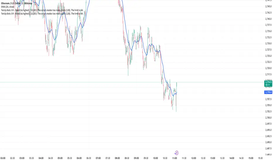
Sentiment Heatmap with EMA Sentiment Heatmap with EMA Let’s build a script mini-LuxAlgo-style sentiment heatmap Enhanced Simple Sentiment Heatmap + Right-Side Legend Automatic legend on the right side
Just like professional indicators:
MAX GREED
GREED
NEUTRAL
FEAR
MAX FEAR
✔ Legend stays updated on the last bar
It moves automatically as price moves.
✔ Trend EMA included (optional) 9 EMA → White
20 EMA → Red
50 EMA → Yellow
100 EMA → Blue
200 EMA → Purple Alerts (e.g., “Max Fear – Buy Zone”)
✔ Liquidity line / support-resistance auto zones Full sentiment heatmap (Greed → Fear)
✔ Right-side legend like LuxAlgo
✔ All 5 EMAs added (my colors): EMA trend cloud (9/20, 20/50, 50/200)
Buy/Sell circles based on sentiment reversals Right-side legend: MAX GREED / GREED / NEUTRAL / FEAR / MAX FEAR
5 EMAs:
9 → White
20 → Red
50 → Yellow
100 → Blue
200 → Purple

MTF MACD – 1m / 15m / 1D / 1W//@version=6
indicator("MTF MACD – 1m / 15m / 1D / 1W", overlay=false)
// MACD inputs
fastLen = input.int(12, "Fast length")
slowLen = input.int(26, "Slow length")
signalLen = input.int(9, "Signal length")
// Multi-timeframe MACD using built-in ta.macd()
= request.security(syminfo.tickerid, "1", ta.macd(close, fastLen, slowLen, signalLen))
= request.security(syminfo.tickerid, "15", ta.macd(close, fastLen, slowLen, signalLen))
= request.security(syminfo.tickerid, "D", ta.macd(close, fastLen, slowLen, signalLen))
= request.security(syminfo.tickerid, "W", ta.macd(close, fastLen, slowLen, signalLen))
// Plot MACD lines for each timeframe
plot(macd_1m, title="MACD 1m", color=color.red, linewidth=2)
plot(macd_15m, title="MACD 15m", color=color.blue, linewidth=2)
plot(macd_1d, title="MACD 1D", color=color.green, linewidth=2)
plot(macd_1w, title="MACD 1W", color=color.orange, linewidth=2)
// (Optional) you can uncomment these if you also want signals/histograms:
// plot(signal_1m, title="Signal 1m", color=color.new(color.red, 50), style=plot.style_dotted)
// plot(signal_15m, title="Signal 15m", color=color.new(color.blue, 50), style=plot.style_dotted)
// plot(signal_1d, title="Signal 1D", color=color.new(color.green, 50), style=plot.style_dotted)
// plot(signal_1w, title="Signal 1W", color=color.new(color.orange, 50), style=plot.style_dotted)
// plot(hist_1m, title="Hist 1m", color=color.red, style=plot.style_histogram)
// plot(hist_15m, title="Hist 15m", color=color.blue, style=plot.style_histogram)
// plot(hist_1d, title="Hist 1D", color=color.green, style=plot.style_histogram)
// plot(hist_1w, title="Hist 1W", color=color.orange, style=plot.style_histogram)
