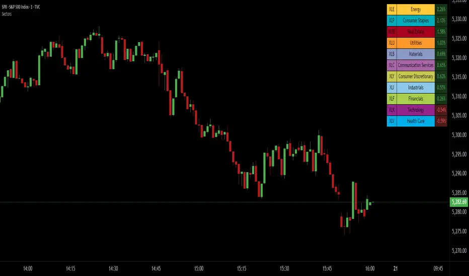
SPDR Sectors TableThis script generates an interactive and customizable SPDR Sectors Table designed to monitor and analyze the performance of the 11 main sectors of the S&P 500 via sector-specific ETFs. It offers a dynamic overview of daily or periodic sector movements, making it a valuable tool for traders, analysts, and investors implementing sector rotation strategies.
█ DEFINITIONS
SPDR Sectors ETFs are exchange-traded funds managed by State Street Global Advisors, which divide the S&P 500 into the following 11 sectors:
- Communication Services (XLC)
- Consumer Discretionary (XLY)
- Consumer Staples (XLP)
- Energy (XLE)
- Financials (XLF)
- Health Care (XLV)
- Industrials (XLI)
- Materials (XLB)
- Real Estate (XLRE)
- Technology (XLK)
- Utilities (XLU)
These ETFs aim to replicate the performance of their respective sectors as defined by the Global Industry Classification Standard (GICS). The funds are periodically rebalanced to match changes in the S&P 500 composition, offering an accurate snapshot of sectoral trends.
█ INDICATOR
The table displays each sector's ticker and full name, following official GICS terminology and SPDR color coding. It also shows percentage performance, calculated daily on intraday charts or based on the selected time frame.
Users can sort the table by either percentage performance or the relative weight of each ETF in the S&P 500. The default weight values reflect data updated as of 17 April 2025, and can be manually adjusted based on the most recent sector weightings available on the official SPDR website.
"电力行业+股票+11年涨幅"に関するスクリプトを検索
Long Term Profitable Swing | AbbasA Story of a Profitable Swing Trading Strategy
Imagine you're sailing across the ocean, looking for the perfect wave to ride. Swing trading is quite similar—you're navigating the stock market, searching for the ideal moments to enter and exit trades. This strategy, created by Abbas, helps you find those waves and ride them effectively to profitable outcomes.
🌊 Finding the Perfect Wave (Entry)
Our journey begins with two simple signs that tell us a great trading opportunity is forming:
- Moving Averages: We use two lines that follow price trends—the faster one (EMA 16) reacts quickly to recent price moves, and the slower one (EMA 30) gives us a longer-term perspective. When the faster line crosses above the slower line, it's like a clear signal saying, "Hey! The wave is rising, and prices might move higher!"
- RSI Momentum: Next, we check a tool called the RSI, which measures momentum (how strongly prices are moving). If the RSI number is above 50, it means there's enough strength behind this rising wave to carry us forward.
When both signals appear together, that's our green light. It's time to jump on our surfboard and start riding this promising wave.
⚓ Safely Riding the Wave (Risk Management)
While we're riding this wave, we want to ensure we're safe from sudden surprises. To do this, we use something called the Average True Range (ATR), which measures how volatile (or bumpy) the price movements are:
- Stop-Loss: To avoid falling too hard, we set a safety line (stop-loss) 8 times the ATR below our entry price. This helps ensure we exit if the wave suddenly turns against us, protecting us from heavy losses.
- Take Profit: We also set a goal to exit the trade at 11 times the ATR above our entry. This way, we capture significant profits when the wave reaches a nice high point.
🌟 Multiple Rides, Bigger Adventures
This strategy allows us to take multiple positions simultaneously—like riding several waves at once, up to 5. Each trade we make uses only 10% of our trading capital, keeping risks manageable and giving us multiple opportunities to win big.
🗺️ Easy to Follow Settings
Here are the basic settings we use:
- Fast EMA**: 16
- Slow EMA**: 30
- RSI Length**: 9
- RSI Threshold**: 50
- ATR Length**: 21
- ATR Stop-Loss Multiplier**: 8
- ATR Take-Profit Multiplier**: 11
These settings are flexible—you can adjust them to better suit different markets or your personal trading style.
🎉 Riding the Waves of Success
This simple yet powerful swing trading approach helps you confidently enter trades, clearly know when to exit, and effectively manage your risk. It’s a reliable way to ride market waves, capture profits, and minimize losses.
Happy trading, and may you find many profitable waves to ride! 🌊✨
Please test, and take into account that it depends on taking multiple longs within the swing, and you only get to invest 25/30% of your equity.

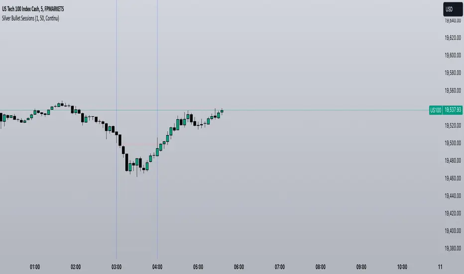
Silver Bullet SessionsThe Silver Bullet Sessions indicator is a specialized timing tool designed to highlight key market sessions throughout the trading day. By marking specific hours with vertical lines, it helps traders identify potentially significant market moments that often coincide with increased volatility and trading opportunities.
This indicator plots vertical lines at six strategic times during the trading day: 3:00 AM, 4:00 AM, 10:00 AM, 11:00 AM, 2:00 PM, and 3:00 PM. These times are carefully selected to correspond with important market events and session overlaps in the global trading cycle. The early morning hours (3-4 AM) often capture significant Asian market movements and the European market opening. The mid-morning period (10-11 AM) typically corresponds with peak European trading hours and the pre-US market dynamics. The afternoon times (2-3 PM) coincide with key US market activities and the European market close.
The indicator is implemented using Pine Script version 6, ensuring compatibility with the latest TradingView platform features. It employs a clean, efficient coding structure that minimizes resource usage while maintaining reliable performance. The vertical lines are rendered in blue for clear visibility against any chart background, and their width is optimized for easy identification without obscuring price action.
Traders can use these visual markers to:
Plan their entries and exits around these key time periods
Anticipate potential market volatility
Structure their trading sessions around these significant market hours
Identify session-based trading patterns
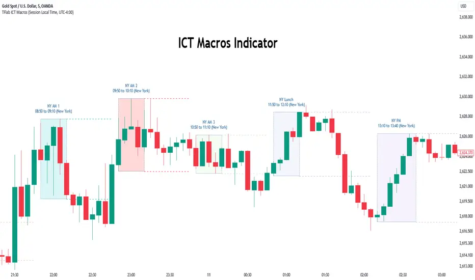
Macros ICT KillZones [TradingFinder] Times & Price Trading Setup🔵 Introduction
ICT Macros, developed by Michael Huddleston, also known as ICT (Inner Circle Trader), is a powerful trading tool designed to help traders identify the best trading opportunities during key time intervals like the London and New York trading sessions.
For traders aiming to capitalize on market volatility, liquidity shifts, and Fair Value Gaps (FVG), understanding and using these critical time zones can significantly improve trading outcomes.
In today’s highly competitive financial markets, identifying the moments when the market is seeking buy-side or sell-side liquidity, or filling price imbalances, is essential for maximizing profitability.
The ICT Macros indicator is built on the renowned ICT time and price theory, which enables traders to track and leverage key market dynamics such as breaks of highs and lows, imbalances, and liquidity hunts.
This indicator automatically detects crucial market times and optimizes strategies for traders by highlighting the specific moments when price movements are most likely to occur. A standout feature of ICT Macros is its automatic adjustment for Daylight Saving Time (DST), ensuring that traders remain synced with the correct session times.
This means you can rely on accurate market timing without the need for manual updates, allowing you to focus on capturing profitable trades during critical timeframes.
🔵 How to Use
The ICT Macros indicator helps you capitalize on trading opportunities during key market moments, particularly when the market is breaking highs or lows, filling Fair Value Gaps (FVG), or addressing imbalances. This indicator is particularly beneficial for traders who seek to identify liquidity, market volatility, and price imbalances.
🟣 Sessions
London Sessions
London Macro 1 :
UTC Time : 06:33 to 07:00
New York Time : 02:33 to 03:00
London Macro 2 :
UTC Time : 08:03 to 08:30
New York Time : 04:03 to 04:30
New York Sessions
New York Macro AM 1 :
UTC Time : 12:50 to 13:10
New York Time : 08:50 to 09:10
New York Macro AM 2 :
UTC Time : 13:50 to 14:10
New York Time : 09:50 to 10:10
New York Macro AM 3 :
UTC Time : 14:50 to 15:10
New York Time : 10:50 to 11:10
New York Lunch Macro :
UTC Time : 15:50 to 16:10
New York Time : 11:50 to 12:10
New York PM Macro :
UTC Time : 17:10 to 17:40
New York Time : 13:10 to 13:40
New York Last Hour Macro :
UTC Time : 19:15 to 19:45
New York Time : 15:15 to 15:45
These time intervals adjust automatically based on Daylight Saving Time (DST), helping traders to enter or exit trades during key market moments when price volatility is high.
Below are the main applications of this tool and how to incorporate it into your trading strategies :
🟣 Combining ICT Macros with Trading Strategies
The ICT Macros indicator can easily be used in conjunction with various trading strategies. Two well-known strategies that can be combined with this indicator include:
ICT 2022 Trading Model : This model is designed based on identifying market liquidity, structural price changes, and Fair Value Gaps (FVG). By using ICT Macros, you can identify the key time intervals when the market is seeking liquidity, filling imbalances, or breaking through important highs and lows, allowing you to enter or exit trades at the right moment.
Silver Bullet Strategy : This strategy, which is built around liquidity hunting and rapid price movements, can work more accurately with the help of ICT Macros. The indicator pinpoints precise liquidity times, helping traders take advantage of market shifts caused by filling Fair Value Gaps or correcting imbalances.
🟣 Capitalizing on Price Volatility During Key Times
Large market algorithms often seek liquidity or fill Fair Value Gaps (FVG) during the intervals marked by ICT Macros. These periods are when price volatility increases, and traders can use these moments to enter or exit trades.
For example, if sell-side liquidity is drained and the market fills an imbalance, the price might move toward buy-side liquidity. By identifying these moments, which may also involve breaking a previous high or low, you can leverage rapid market fluctuations to your advantage.
🟣 Identifying Liquidity and Price Imbalances
One of the important uses of ICT Macros is identifying points where the market is seeking liquidity and correcting imbalances. You can determine high or low liquidity levels in the market before each ICT Macro, as well as Fair Value Gaps (FVG) and price imbalances that need to be filled, using them to adjust your trading strategy. This capability allows you to manage trades based on liquidity shifts or imbalance corrections without needing a bias toward a specific direction.
🔵 Settings
The ICT Macros indicator offers various customization options, allowing users to tailor it to their specific needs. Below are the main settings:
Time Zone Mode : You can select one of the following options to define how time is displayed:
UTC : For traders who need to work with Universal Time.
Session Local Time : The local time corresponding to the London or New York markets.
Your Time Zone : You can specify your own time zone (e.g., "UTC-4:00").
Your Time Zone : If you choose "Your Time Zone," you can set your specific time zone. By default, this is set to UTC-4:00.
Show Range Time : This option allows you to display the time range of each session on the chart. If enabled, the exact start and end times of each interval are shown.
Show or Hide Time Ranges : Toggle on/off for visual clarity depending on user preference.
Custom Colors : Set distinct colors for each session, allowing users to personalize their chart based on their trading style.These settings allow you to adjust the key time intervals of each trading session to your preference and customize the time format according to your own needs.
🔵 Conclusion
The ICT Macros indicator is a powerful tool for traders, helping them to identify key time intervals where the market seeks liquidity or fills Fair Value Gaps (FVG), corrects imbalances, and breaks highs or lows. This tool is especially valuable for traders using liquidity-based strategies such as ICT 2022 or Silver Bullet.
One of the key features of this indicator is its support for Daylight Saving Time (DST), ensuring you are always in sync with the correct trading session timings without manual adjustments. This is particularly beneficial for traders operating across different time zones.
With ICT Macros, you can capitalize on crucial market opportunities during sensitive times, take advantage of imbalances, and enhance your trading strategies based on market volatility, liquidity shifts, and Fair Value Gaps.
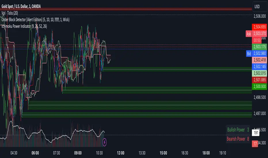
Ichimoku Power Indicator# Ichimoku Power Indicator
## Overview
The Ichimoku Power Indicator is an advanced tool that combines the traditional Ichimoku Cloud system with a unique power ranking mechanism. This indicator provides traders with a comprehensive view of market trends and potential reversal points, all while quantifying the strength of bullish and bearish signals.
## Key Features
1. **Full Ichimoku Cloud Visualization:** Displays all components of the Ichimoku Cloud system, including Conversion Line (Tenkan-sen), Base Line (Kijun-sen), Leading Span A and B (Kumo), and Lagging Span (Chikou Span).
2. **Power Ranking System:** Calculates and displays a bullish and bearish power score based on 11 different Ichimoku-derived conditions.
3. **Real-time Updates:** Power scores are updated in real-time as market conditions change.
4. **Easy-to-Read Display:** A clear, color-coded table shows the current bullish and bearish power scores.
5. **Customizable Parameters:** Allows adjustment of key Ichimoku settings to suit different trading styles and timeframes.
## How It Works
The indicator evaluates 11 different conditions derived from Ichimoku Cloud components:
1. Cloud color
2. Price position relative to the cloud
3. Tenkan-sen vs Kijun-sen
4. Price vs Tenkan-sen
5. Price vs Kijun-sen
6. Tenkan-sen vs Cloud
7. Kijun-sen vs Cloud
8. Chikou Span vs Cloud
9. Chikou Span vs Tenkan-sen
10. Chikou Span vs Kijun-sen
11. Chikou Span vs Price
Each bullish condition adds a point to the bullish power score, while each bearish condition adds a point to the bearish power score. The maximum score for each is 11.
## Interpretation
- Higher bullish scores suggest stronger upward trends or potential bullish reversals.
- Higher bearish scores indicate stronger downward trends or potential bearish reversals.
- When scores are close, it may indicate a period of consolidation or uncertainty.
## Use Cases
- Trend Confirmation: Use in conjunction with price action to confirm the strength of current trends.
- Reversal Detection: Watch for changes in power scores as early indicators of potential trend reversals.
- Entry and Exit Signals: High power scores can be used to identify optimal entry or exit points.
- Market Analysis: Gain a quick overview of market conditions across multiple assets or timeframes.
## Note
This indicator is designed to complement your existing trading strategy. Always use it in conjunction with other forms of analysis and proper risk management techniques.
Experiment with different timeframes and settings to find the configuration that best suits your trading style and the assets you trade.
Happy trading!
Daily Levels Percentual [TOLK] Settings Crypto and ForexPercentage zones refer to specific areas or bands on the price chart of a financial asset that are bounded by percentages of change relative to a reference point, such as the opening price or a reference value from a previous move.
These zones are useful for identifying support and resistance levels, predicting possible price reversals, or setting price targets. For example, on a price chart, you can create percentage zones to observe how the price behaves when it reaches 1%, 2%, 5%, 10%, etc., above or below a certain point.
These zones can be used in conjunction with other technical analysis tools, such as Fibonacci, moving averages, or volume analysis, to improve decision-making in trading strategies.
The default indicator levels are as follows:
SETTINGS Crypto:
Crypto Level 1 > 1.0%
Crypto Level 2 > 1.618%
Crypto Level 3 > 2.0%
Crypto Level 4 > 2.618%
Crypto Level 5 > 3.618%
Crypto Level 6 > 4.618%
Crypto Level 7 > 5.0%
Crypto Level 8 > 7.618%
Crypto Level 9 > 10.0%
Crypto Level 10 > 12.618%
Crypto Level 11 > 13.618%
Crypto Level 12 > 15%
Crypto Level 13 > 17.618%
Crypto Level 14 > 20%
SETTINGS Forex:
Forex Level 1 > 0.10%
Forex Level 2 > 0.1618%
Forex Level 3 > 0.20%
Forex Level 4 > 0.2618%
Forex Level 5 > 0.3618%
Forex Level 6 > 0.4618%
Forex Level 7 > 0.50%
Forex Level 8 > 0.7618%
Forex Level 9 > 1.0%
Forex Level 10 > 1.2618%
Forex Level 11 > 1.3618%
Forex Level 12 > 1.50%
Forex Level 13 > 1.7618%
Forex Level 14 > 2.0%
Percentage Levels This approach helps identify critical price levels where the asset may encounter support or resistance, making it easier to make trading decisions based on price movement patterns.

Macro Times [Blu_Ju]About ICT Macro Times:
The Inner Circle Trader (ICT) has taught that there are certain time sessions when the Interbank Price Delivery Algorithm (IPDA) is running a macro. The macro itself could be a repricing macro, a consolidation macro, etc. - this depends on where price currently is in relation to its draw. The times the macro is active do not change however, and are always the following (in New York local time):
8:50-9:10 (premarket macro)
9:50-10:10 (AM macro 1)
10:50-11:10 (AM macro 2)
11:50-12:10 (lunch macro)
13:10-13:40 (PM macro)
15:15-15:45 (final hour macro)
Because these times are fixed, traders can anticipate a setup is likely to form in or around these sessions. Setups may involve sweeps of liquidity (highs/lows), repricing to inefficiencies (e.g., fair value gaps), breaker setups, etc. (The specific setup involved is beyond the scope of this script; this script is concerned with visually marking the time sessions only.)
About this Script:
The scope of this script is to visually identify the macro active time sessions. This script draws vertical lines to mark the start and end of the macro time sessions. Optionally, the user can use a background color for the macro session with or without the vertical lines. The user can also toggle on or off any of the macro sessions, if he or she is only interested in certain ones. The user also has the freedom to change the times of the macro sessions if he or she is interested in a different time.
What makes this script unique is that it plots the macro time sessions after midnight for each day, before the real-time bar reaches the macro times. This is advantageous to the trader, as it gives the trader a visual cue that the macro times are approaching. When watching price it is easy to lose track of time, and the purpose of this script is to help the trader maintain where price is in relation to the macro time sessions in a simple, visual way.

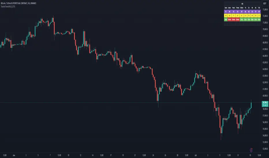
TechniTrend RSI (11TF)Multi-Timeframe RSI Indicator
Overview
The Multi-Timeframe RSI Indicator is a sophisticated tool designed to provide comprehensive insights into the Relative Strength Index (RSI) across 11 different timeframes simultaneously. This indicator is essential for traders who wish to monitor RSI trends and their moving averages (MA) to make informed trading decisions.
Features
Multiple Timeframes: Displays RSI and RSI MA values for 11 different timeframes, allowing traders to have a holistic view of the market conditions.
RSI vs. MA Comparison: Indicates whether the RSI value is above or below its moving average for each timeframe, helping traders to identify bullish or bearish momentum.
Overbought/Oversold Signals:
Marks "OS" (OverSell) when RSI falls below 25, indicating a potential oversold condition.
Marks "OB" (OverBuy) when RSI exceeds 75, signaling a potential overbought condition.
Real-Time Updates: Continuously updates in real-time to provide the most current market information.
Usage
This indicator is invaluable for traders who utilize RSI as part of their technical analysis strategy. By monitoring multiple timeframes, traders can:
Identify key overbought and oversold levels to make entry and exit decisions.
Observe the momentum shifts indicated by RSI crossing above or below its moving average.
Enhance their trading strategy by integrating multi-timeframe analysis for better accuracy and confirmation.
How to Interpret the Indicator
RSI Above MA: Indicates a potential bullish trend. Traders may consider looking for long positions.
RSI Below MA: Suggests a potential bearish trend. Traders may look for short positions.
OS (OverSell): When RSI < 25, the market may be oversold, presenting potential buying opportunities.
OB (OverBuy): When RSI > 75, the market may be overbought, indicating potential selling opportunities.
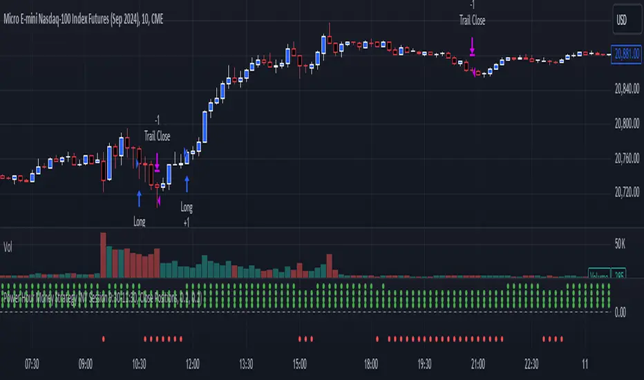
Power Hour Money StrategyDescription of the Pine Script Code: "Power Hour Money Strategy"
This Pine Script strategy, "Power Hour Money Strategy," is designed to trade based on the alignment of multiple time frames (month, week, day, and hour). The strategy aims to enter long or short positions depending on whether all selected time frames are in sync (all green for long positions, all red for short positions). Additionally, the script includes configurations for trading during specific sessions and automatically closing positions at the end of the trading day.
Core Features:
1. Time Frame Sync Check:
- The strategy evaluates whether the current price is higher than the opening price for the month, week, day, and hour to determine if each time frame is "green" (bullish) or "red" (bearish).
2. Session Control:
- The user can select between different trading sessions:
- "NY Session 9:30-11:30"
- "Extended NY Session 8-4"
- "All Sessions"
- Trades are only executed if the current time falls within the selected session.
3. Trailing Stop Mechanism:
- The strategy includes an optional trailing stop mechanism for both long and short positions.
- The trailing stop is configured with a percentage loss from the current price to protect gains.
4. End-of-Day Position Management:
- An option is provided to automatically close all positions at the end of the trading day (5:45 PM Eastern Time).
Detailed Code Breakdown:
1. Input Settings:
- **Session Selection**: Allows the user to choose the trading session.
- **End-of-Day Close**: Option to automatically close positions at the end of the day.
- **Trailing Stop Loss**: Enables or disables the trailing stop loss feature and sets the percentage for long and short positions.
2. Time Frame Calculations:
- The script uses `request.security` to get the opening prices for higher time frames (monthly, weekly, daily, and hourly).
- It compares the current close price to these opening prices to determine if each time frame is green or red.
3. Session Time Definitions:
- Defines the start and end times for the NY session (9:30-11:30 AM) and the extended session (8:00 AM - 4:00 PM).
4. Trade Execution:
- The strategy checks if all selected time frames are in sync and if the current time falls within the trading session.
- If all conditions are met, it enters a long or short position.
5. Trailing Stop Loss Implementation:
- Adjusts the stop price based on the trailing percentage and the current position's size.
- Automatically exits positions if the trailing stop condition is met.
6. End-of-Day Close Implementation:
- Uses a timestamp to check if the current time is 5:45 PM Eastern Time.
- Closes all positions if the end-of-day condition is met.
7. Plotting and Logging:
- Plots indicators to visualize the green/red status of each time frame.
- Logs information about the status of each time frame for debugging and analysis.
Example Usage:
Entering a Long Position: If the month, week, day, and hour are all green and the current time is within the selected session, a long position is entered.
Entering a Short Position: If the month, week, day, and hour are all red and the current time is within the selected session, a short position is entered.
Trailing Stop: Protects gains by exiting the position if the price moves against the set trailing stop percentage.
End-of-Day Close: Automatically closes all open positions at 5:45 PM Eastern Time if enabled.
This strategy is particularly useful for traders who want to ensure that multiple time frames are in alignment before entering a trade and who wish to manage positions effectively throughout the trading day with specific session controls and trailing stops.
NASDAQ 100 Peak Hours StrategyNASDAQ 100 Peak Hours Trading Strategy
Description
Our NASDAQ 100 Peak Hours Trading Strategy leverages a carefully designed algorithm to trade within specific hours of high market activity, particularly focusing on the first two hours of the trading session from 09:30 AM to 11:30 AM GMT-5. This period is identified for its increased volatility and liquidity, offering numerous trading opportunities.
The strategy incorporates a blend of technical indicators to identify entry and exit points for both long and short positions. These indicators include:
Exponential Moving Averages (EMAs) : A short-term 9-period EMA and a longer-term 21-period EMA to determine the market trend and momentum.
Relative Strength Index (RSI) : A 14-period RSI to gauge the market's momentum.
Average True Range (ATR) : A 14-period ATR to assess market volatility and to set dynamic stop losses and trailing stops.
Volume Weighted Average Price (VWAP) : To identify the market's average price weighted by volume, serving as a benchmark for the trading day.
Our strategy uniquely applies a volatility filter using the ATR, ensuring trades are only executed in conditions that favor our setup. Additionally, we consider the direction of the EMAs to confirm the market's trend before entering trades.
Originality and Usefulness
This strategy stands out by combining these indicators within the NASDAQ 100's peak hours, exploiting the specific market conditions that prevail during these times. The inclusion of a volatility filter and dynamic stop-loss mechanisms based on the ATR provides a robust method for managing risk.
By focusing on the early trading hours, the strategy aims to capture the initial market movements driven by overnight news and the opening rush, often characterized by higher volatility. This approach is particularly useful for traders looking to maximize gains from short-term fluctuations while limiting exposure to longer-term market uncertainty.
Strategy Results
To ensure the strategy's effectiveness and reliability, it has undergone rigorous backtesting over a significant dataset to produce a sample size of more than 100 trades. This testing phase helps in identifying the strategy's potential in various market conditions, its consistency, and its risk-to-reward ratio.
Our backtesting adheres to realistic trading conditions, accounting for slippage and commission to reflect actual trading scenarios accurately. The strategy is designed with a conservative approach to risk management, advising not to risk more than 5-10% of equity on a single trade. The default settings in the script align with these principles, ensuring that users can replicate our tested conditions.
Using the Strategy
The strategy is designed for simplicity and ease of use:
Trade Hours : Focuses on 09:30 AM to 11:30 AM GMT-5, during the NASDAQ 100's peak activity hours.
Entry Conditions : Trades are initiated based on the alignment of EMAs, RSI, VWAP, and the ATR's volatility filter within the designated time frame.
Exit Conditions : Includes dynamic trailing stops based on ATR, a predefined time exit strategy, and a trend reversal exit condition for risk management.
This script is a powerful tool for traders looking to leverage the NASDAQ 100's peak hours, providing a structured approach to navigating the early market hours with a robust set of criteria for making informed trading decisions.

Time Based Comparison Tool [TFO]The goal of this indicator is to show how multiple assets are trading relative to their Previous Highs and Lows. Many traders have probably seen charts resembling this that may plot how asset prices are trading as a percent change over time, or something similar.
The key difference with this indicator is that all prices are normalized to reflect how they are trading with respect to the previous range of a user-defined timeframe. Without the normalization process, we would simply be observing some percent change from a given point in time; but this does not provide enough information to describe where price is trading relative to our desired frame of reference.
For example, if the timeframe setting was chosen to be 1 day, the indicator would plot the Previous High (PH) and Previous Low (PL) of the current symbol on the daily timeframe, denoted here by the black lines and labels. Then, the adjusted price of all selected symbols would be shown to visualize how each one is moving with respect its own PH and PL, using the current symbol's PH and PL as reference points.
In the above chart, we can see that CL was trading below its PDL from about 10:00-11:00 am EST, then broke above and retested it at around 11:20 am EST, before trading higher. To verify that this comparison works as intended, we can check to see that CL did in fact retest its PDL at this time before trading higher. Note that we are using the close price for this evaluation.
Since limiting the output to close prices can leave out some vital information, we can change the Plot Type setting from "Close" to "High to Low," which will instead show the range of prices from high to low instead of just the close.
We can expand on this by detecting when PH's and PL's have been raided (traded through), by displaying the text PHR (Previous High Raid) or PLR (Previous Low Raid) next to the symbol's label on the right. In this case below, where we're using the 1 week timeframe, we can observe that NQ1! (purple) traded through the PL level and thus its label (right) is updated to indicate a PLR.
Similarly, YM1! traded through its PH level and was updated to indicate a PHR; and ES1! raided both levels, with its label reflecting just that.
Due to the native limitation of output series in a single pine script, alerts have been consolidated to "Any PHR" or "Any PLR," meaning these alerts would fire if any of the selected symbols raided a PH or PL, respectively. If one wanted to be alerted for just a specific symbol, this could be achieved by deselecting all symbols except that which is desired, then setting an alert and adjusting its title for easier user recognition.

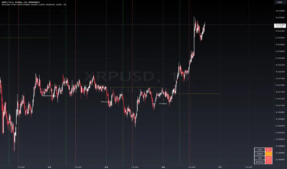
Master Fren Jedi HelperDescription:
The "Master Fren Jedi Helper" is a TradingView indicator designed to enhance trading analysis by plotting distinct lines at crucial times of the trading day.
This indicator is an invaluable tool for traders who focus on intraday price movements and patterns around specific times. Its primary features include:
Customizable Time Markers: The script allows users to mark specific times of the day with lines of different colors and styles. These times are adjustable based on the user's timezone and preferences.
Configurable Line Properties: Users can customize the color and style of each line. The script offers options for a green line at 7 AM, a red line at 11 AM, a grey line at midnight, and a yelow line to denote the daily open.
Time Zone Adjustment: To work with New York time zone, you have ability to adjust for different time zones. Users can input their time zone offset, advised to use UTC -5 allowing the script to plot the lines accurately according to their local time.
Day Labels: The indicator also labels each day of the week at midnight, providing a clear and easy way to track the days on the chart.
Functionality Overview:
Green Line at 7 AM: This line helps identify the early morning market sentiment. Users can customize the color and style of this line.
Red Line at 11 AM: Plotted to highlight mid-morning price levels, this line is also customizable in color and style.
Grey Line at Midnight: Marks the start of a new trading day. The line style and color can be personalized.
Yellow Line for Daily Open: Indicates the opening price of the day. The line's color and style are adjustable.
Time Zone Configuration: Users can set their local time zone to ensure the lines correspond accurately with their specific market hours.
Day of the Week Labels: Each midnight is labeled with the day of the week, aiding in the weekly analysis of price patterns.
This indicator is perfect for traders who need to quickly identify key times and price levels each day. It's easily configurable to suit various trading strategies and assists in enhancing the visual representation of intraday market dynamics.
Cycles 90mThe cycles are separated by vertical lines. The first cycle (Q1) is marked with a red line because it is a manipulative cycle where you should not open positions. Other cycles are green (Q2, Q3, Q4).
You can add the time of the current candle, its size and position on the chart in the settings
The time is highlighted in red in the timeframes 9:30-9:40, 10:00-10:10, 11:00-11:30, 15:30-15:40, 16:00-16:10, 17:00-17:10, 17:30-17:40, as price movements are most often expected during these timeframes.
The cycle lines automatically disappear if you open a timeframe above M15

savitzkyGolay, KAMA, HPOverview
This trading indicator integrates three distinct analytical tools: the Savitzky-Golay Filter, Kaufman Adaptive Moving Average (KAMA), and Hodrick-Prescott (HP) Filter. It is designed to provide a comprehensive analysis of market trends and potential trading signals.
Components
Hodrick-Prescott (HP) Filter
Purpose: Smooths out the price data to identify the underlying trend.
Parameters: Lambda: Controls the smoothness. Range: 50 to 1600.
Impact of Parameters:
Increasing Lambda: This makes the trend line more responsive to short-term market fluctuations, suitable for short-term analysis. A higher Lambda value decreases the degree of smoothing, making the trend line follow recent market movements more closely.
Decreasing Lambda: A lower Lambda value makes the trend line smoother and less responsive to short-term market fluctuations, ideal for longer-term trend analysis. Decreasing Lambda increases the degree of smoothing, thereby filtering out minor market movements and focusing more on the long-term trend.
Kaufman Adaptive Moving Average (KAMA):
Purpose: An adaptive moving average that adjusts to price volatility.
Parameters: Length, Fast Length, Slow Length: Define the sensitivity and adaptiveness of KAMA.
Impact of Parameters:
Adjusting Length affects the base period for efficiency ratio, altering the overall sensitivity.
Fast Length and Slow Length control the speed of KAMA’s adaptation. A smaller Fast Length makes KAMA more sensitive to price changes, while a larger Slow Length makes it less sensitive.
Savitzky-Golay Filter:
Purpose: Smooths the price data using polynomial regression.
Parameters: Window Size: Determines the size of the moving window (7, 9, 11, 15, 21).
Impact of Parameters:
A larger Window Size results in a smoother curve, which is more effective for identifying long-term trends but can delay reaction to recent market changes.
A smaller Window Size makes the curve more responsive to short-term price movements, suitable for short-term trading strategies.
General Impact of Parameters
Adjusting these parameters can significantly alter the signals generated by the indicator. Users should fine-tune these settings based on their trading style, the characteristics of the traded asset, and market conditions to optimize the indicator's performance.
Signal Logic
Buy Signal: The trend from the HP filter is below both the KAMA and the Savitzky-Golay SMA, and none of these indicators are flat.
Sell Signal: The trend from the HP filter is above both the KAMA and the Savitzky-Golay SMA, and none of these indicators are flat.
Usage
Due to the combination of smoothing algorithms and adaptability, this indicator is highly effective at identifying emerging trends for both initiating long and short positions.
IMPORTANT : Although the code and user settings incorporate measures to limit false signals due to lateral (sideways) movement, they do not completely eliminate such occurrences. Users are strongly advised to avoid signals that emerge during simultaneous lateral movements of all three indicators.
Despite the indicator's success in historical data analysis using its signals alone, it is highly recommended to use this code in combination with other indicators, patterns, and zones. This is particularly important for determining exit points from positions, which can significantly enhance trading results.
Limitations and Recommendations
The indicator has shown excellent performance on the weekly time frame (TF) with the following settings:
Savitzky-Golay (SG): 11
Hodrick-Prescott (HP): 100
Kaufman Adaptive Moving Average (KAMA): 20, 2, 30
For the monthly TF, the recommended settings are:
SG: 15
HP: 100
KAMA: 30, 2, 35
Note: The monthly TF is quite variable. With these settings, there may be fewer signals, but they tend to be more relevant for long-term investors. Based on a sample of 40 different stocks from various countries and sectors, most exhibited an average trade return in the thousands of percent.
It's important to note that while these settings have been successful in past performance, market conditions vary and past performance is not indicative of future results. Users are encouraged to experiment with these settings and adjust them according to their individual needs and market analysis.
As this is my first developed trading indicator, I am very open to and appreciative of any suggestions or comments. Your feedback is invaluable in helping me refine and improve this tool. Please feel free to share your experiences, insights, or any recommendations you may have.

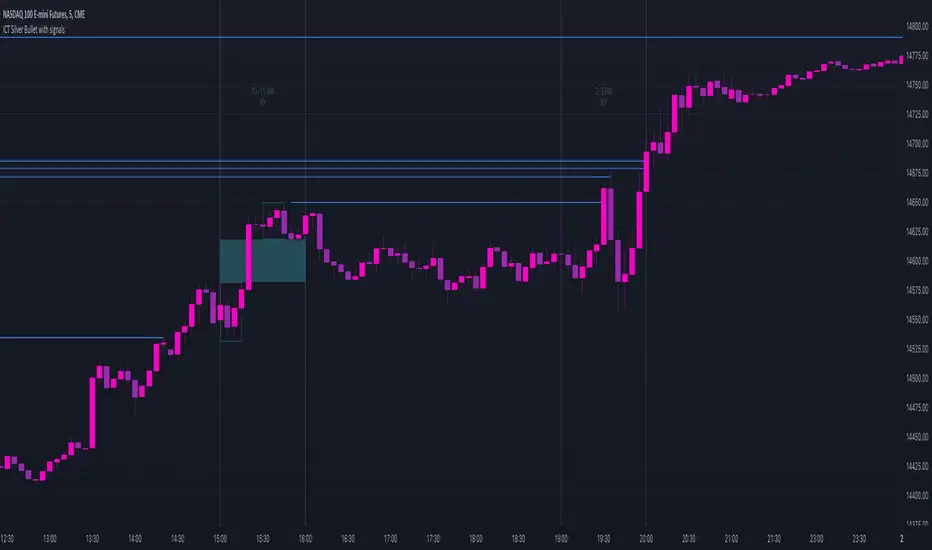
ICT Silver Bullet with signals
The "ICT Silver Bullet with signals" indicator (inspired from the lectures of "The Inner Circle Trader" (ICT)),
goes a step further than the ICT Silver Bullet publication, which I made for LuxAlgo :
• uses HTF candles
• instant drawing of Support & Resistance (S/R) lines when price retraces into FVG
• NWOG - NDOG S/R lines
• signals
The Silver Bullet (SB) window which is a specific 1-hour interval where a Fair Value Gap (FVG) pattern can be formed.
When price goes back to the FVG, without breaking it, Support & Resistance lines will be drawn immediately.
There are 3 different Silver Bullet windows (New York local time):
The London Open Silver Bullet (03 AM — 04 AM ~ 03:00 — 04:00)
The AM Session Silver Bullet (10 AM — 11 AM ~ 10:00 — 11:00)
The PM Session Silver Bullet (02 PM — 03 PM ~ 14:00 — 15:00)
🔶 USAGE
This technique can visualise potential support/resistance lines, which can be used as targets.
The script contains 2 main components:
• forming of a Fair Value Gap (FVG)
• drawing support/resistance (S/R) lines
🔹 Forming of FVG
When HTF candles forms an FVG, the FVG will be drawn at the end (close) of the last HTF candle.
To make it easier to visualise the 2 HTF candles that form the FVG, you can enable
• SHOW -> HTF candles
During the SB session, when a FVG is broken, the FVG will be removed, together with its S/R lines.
The same goes if price did not retrace into FVG at the last bar of the SB session
Only exception is when "Remove broken FVG's" is disabled.
In this case a FVG can be broken, as long as price bounces back before the end of the SB session, it will remain to be visible:
🔹 Drawing support/resistance lines
S/R target lines are drawn immediately when price retraces into the FVG.
They will remain updated until they are broken (target hit)
Potential S/R lines are formed by:
• previous swings (swing settings (left-right)
• New Week Opening Gap (NWOG): close on Friday - weekly open
• New Day Opening Gap (NWOG): close previous day - current daily open
Only non-broken lines are included.
Broken =
• minimum of open and close below potential S/R line
• maximum of open and close above potential S/R line
NDOG lines are coloured fuchsia (as in the ICT lectures), NWOG are coloured white (darkmode) or black (lightmode ~ ICT lectures)
Swing line colour can be set as desired.
Here S/R includes NDOG lines:
The same situation, with "Extend Target-lines to their source" enabled:
Here with NWOG lines:
This publication contains a "Minimum Trade Framework (mTFW)", which represents the best-case expected price delivery, this is not your actual trade entry - exit range.
• 40 ticks for index futures or indices
• 15 pips for Forex pairs
The minimum distance (if applicable) can be shown by enabling "Show" - "Minimum Trade Framework" -> blue arrow from close to mTFW
Potential S/R lines needs to be higher (bullish) or lower (bearish) than mTFW.
🔶 SETTINGS
(check USAGE for deeper insights and explanation)
🔹 Only last x bars: when enabled, the script will do most of the calculations at these last x candles, potentially this can speeds calculations.
🔹 Swing settings (left-right): Sets the length, which will set the lookback period/sensitivity of the ZigZag patterns (which directs the trend and points for S/R lines)
🔹 FVG
HTF (minutes): 1-15 minutes.
• When the chart TF is equal of higher, calculations are based on current TF.
• Chart TF > 15 minutes will give the warning: "Please use a timeframe <= 15 minutes".
Remove broken FVG's: when enabled the script will remove FVG (+ associated S/R lines) immediately when FVG is broken at opposite direction.
FVG's still will be automatically removed at the end of the SB session, when there is no retrace, together with associated S/R lines,...
~ trend: Only include FVG in the same direction as the current trend
Note -> when set 'right' (swing setting) rather high ( > 3), he trend change will be delayed as well (default 'right' max 5)
Extend: extend FVG to max right side of SB session
🔹 Targets – support/resistance
Extend Target-lines to their source: extend lines to their origin
Colours (Swing S/R lines)
🔹 Show
SB session: show lines and labels of SB session (+ colour)
• Labels can be disabled separately in the 'Style' section, colour is set at the 'Inputs' section
Trend : Show trend (ZigZag, coloured ~ trend)
HTF candles: Show the 2 HTF candles that form the FVG
Minimum Trade Framework: blue arrow (if applicable)
🔶 ALERTS
There are 4 signals provided (bullish/bearish):
FVG Formed
FVG Retrace
Target reached
FVG cancelled
You can choose between dynamic alerts - only 1 alert needs to be set for all signals, or you can set specific alerts as desired.
💜 PURPLE BARS 😈
• Since TradingView has chosen to give away our precious Purple coloured Wizard Badge, bars are coloured purple 😊😉
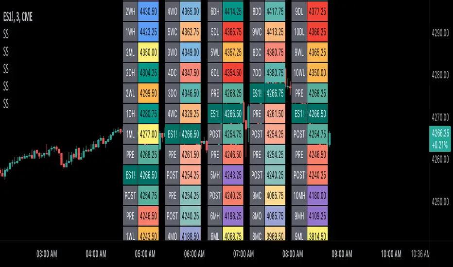
Scoopy StacksWaffle Around Multiple
(Open, High, Low, Close) Stacks On
Pre/Post Market & (Daily, Weekly,
Monthly, Yearly) Sessions With
Meticulous Columns, Rows, Tooltips,
Colors, Custom Ideas, and Alerts.
Sessions Use Two Step Incremental Values
Default Value: (1) Shows Two Previous
(O, H, L, C); Increasing Value Swaps
Sessions With Next Two Stacks.
⬛️ KEY WORDS:
🟢 Crossover | 🔴 Crossunder
📗 High | 📕 Low
📔 Open | 📓 Close
🥇 First Idea | 🥈 Second Idea
🥉 Third Idea | 🎖️ Fourth Idea
🟥 ALERTS:
Default Option: (Per Bar)
Alerts Once Conditions Are Met
(Bar Close) Alerts When Bar Closes
Default Option: (Reg)
Alerts During Regular Market
Trading Hours, (0930-1600)
(Ext) Alerts During Extended
Market Hours, (1600-0930)
(24/7) Alerts All Day
Optional Preferences:
Regular Alerts - Stocks
Extended Alerts - Futures
24/7 Alerts - Crypto
🟧 STACKS:
Default Value: (1)
Incremental Stack Value, Increasing Value
Swaps Sessions With the Next Two Stacks
(✓) Swap Stacks?
Pre/Post Market High/Lows,
1-2 Day High/Lows, 1-2 Week High/Lows,
1-2 Month High/Lows, 1-2 Year High/Lows
( ) Swap Stacks?
Pre/Post Market Open/Close,
1-2 Day Open/Close, 1-2 Week Open/Close,
1-2 Month Open/Close, 1-2 Year Open/Close
🟨 EXAMPLES:
Default Stack:
🟢 | 📗 Pre Market High (PRE) | 4600.00
🔴 | 📕 Post Market Low (POST) | 420.00
Optional: (Open)
🟢 | 📔 Post Market Open (POST) | 4400.00
Optional: (Close)
🔴 | 📓 Pre Market Close (PRE) | 430.00
Default Stack Value: (1)
🔴 | 📗 1 Day High (1DH) | 460.00
Next Stack Value: (3)
🟢 | 📕 4 Day Low (4DL) | 420.00
Optional: (Open)
🔴 | 📔 2 Day Open (2DO) | 440.00
Optional: (Close)
🟢 | 📓 3 Day Close (3DC) | 430.00
Default Stack Value: (5)
🟢 | 📗 5 Week High (5WH) | 460.00
Next Stack Value: (7)
🔴 | 📕 8 Week Low (8WL) | 420.00
Optional: (Open)
🔴 | 📔 7 Week Open (7WO) | 4400.00
Optional: (Close)
🟢 | 📓 6 Week Close (6WC) | 430.00
Default Stack Value: (9)
🔴 | 📗 9 Month High (9MH) | 460.00
Next Stack Value: (11)
🟢 | 📕 12 Month Low (12ML) | 420.00
Optional: (Open)
🟢 | 📔 11 Month Open (11MO) | 4400.00
Optional: (Close)
🔴 | 📓 10 Month Close (10MC) | 430.00
Default Stack Value: (13)
🟢 | 📗 13 Year High (13YH) | 460.00
Next Stack Value: (15)
🟢 | 📕 16 Year Low (16YL) | 420.00
Optional: (Open)
🔴 | 📔 15 Year Open (15YO) | 4400.00
Optional: (Close)
🔴 | 📓 14 Year Close (14YC) | 430.00
🟩 TABLES:
Default Value: (1)
Moves Table Up, Down, Left, or Right
Based on Second Default Value
First Default Value: (Top Right)
Sets Table Placement, Middle Center
Allows Table To Move In All Directions
Second Default Value: (Default)
Fixed Table Position, Switching Values
Moves Direction of the Table
🟦 IDEAS:
(✓) Show Ideas?
Shows Four Ideas With Custom Texts
and Values; Ideas Are Based Around
Post-It Note Reminders with Alerts
Suggestions For Text Ideas:
Take Profit, Stop Loss, Trim, Hold,
Long, Short, Bounce Spot, Retest,
Chop, Support, Resistance, Buy, Sell
🟪 EXAMPLES:
Default Value: (5)
Shows the Custom Table Value For
Sorted Table Positions and Alerts
Default Text: (🥇)
Shown On First Table Cell and
Message Appearing On Alerts
Alert Shows: 🟢 | 🥇 | 5.00
Default Value: (10)
Shows the Custom Table Value For
Sorted Table Positions and Alerts
Default Text: (🥈)
Shown On Second Table Cell and
Message Appearing On Alerts
Alert Shows: 🔴 | 🥈 | 10.00
Default Value: (50)
Shows the Custom Table Value For
Sorted Table Positions and Alerts
Default Text: (🥉)
Shown On Third Table Cell and
Message Appearing On Alerts
Alert Shows: 🟢 | 🥉 | 50.00
Default Value: (100)
Shows the Custom Table Value For
Sorted Table Positions and Alerts
Default Text: (🎖️)
Shown On Fourth Table Cell and
Message Appearing On Alerts
Alert Shows: 🔴 | 🎖️ | 100.00
⬛️ REFERENCES:
Pre-market Highs & Lows on regular
trading hours (RTH) chart
By Twingall
Previous Day Week Highs & Lows
By Sbtnc
Screener for 40+ instruments
By QuantNomad
Daily Weekly Monthly Yearly Opens
By Meliksah55
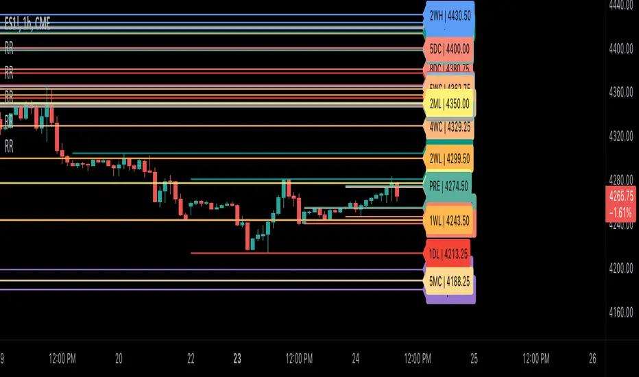
Ribbit RangesBounce Around Multiple
(Open, High, Low, Close) Ranges
On Pre/Post Market & (Daily, Weekly,
Monthly, Yearly) Sessions With
Meticulous Lines, Labels, Tooltips,
Colors, Custom Ideas, and Alerts.
Sessions Use Two Step Incremental Values
Default Value: (1) Shows Two Previous
(O, H, L, C); Increasing Value Swaps
Sessions With Next Two Ranges.
⬛️ KEY WORDS:
🟢 Crossover | 🔴 Crossunder
📗 High | 📕 Low
📔 Open | 📓 Close
🥇 First Idea | 🥈 Second Idea
🥉 Third Idea | 🎖️ Fourth Idea
🟥 ALERTS:
Default Option: (Per Bar)
Alerts Once Conditions Are Met
(Bar Close) Alerts When Bar Closes
Default Option: (Reg)
Alerts During Regular Market
Trading Hours, (0930-1600)
(Ext) Alerts During Extended
Market Hours, (1600-0930)
(24/7) Alerts All Day
Optional Preferences:
Regular Alerts - Stocks
Extended Alerts - Futures
24/7 Alerts - Crypto
🟧 RANGES:
Default Value: (1)
Incremental Range Value, Increasing Value
Swaps Sessions With the Next Two Ranges
(✓) Swap Ranges?
Pre/Post Market High/Lows,
1-2 Day High/Lows, 1-2 Week High/Lows,
1-2 Month High/Lows, 1-2 Year High/Lows
( ) Swap Ranges?
Pre/Post Market Open/Close,
1-2 Day Open/Close, 1-2 Week Open/Close,
1-2 Month Open/Close, 1-2 Year Open/Close
🟨 EXAMPLES:
Default Range:
🟢 | 📗 Pre Market High (PRE) | 4600.00
🔴 | 📕 Post Market Low (POST) | 420.00
Optional: (Open)
🟢 | 📔 Post Market Open (POST) | 4400.00
Optional: (Close)
🔴 | 📓 Pre Market Close (PRE) | 430.00
Default Range Value: (1)
🔴 | 📗 1 Day High (1DH) | 460.00
Next Range Value: (3)
🟢 | 📕 4 Day Low (4DL) | 420.00
Optional: (Open)
🔴 | 📔 2 Day Open (2DO) | 440.00
Optional: (Close)
🟢 | 📓 3 Day Close (3DC) | 430.00
Default Range Value: (5)
🟢 | 📗 5 Week High (5WH) | 460.00
Next Range Value: (7)
🔴 | 📕 8 Week Low (8WL) | 420.00
Optional: (Open)
🔴 | 📔 7 Week Open (7WO) | 4400.00
Optional: (Close)
🟢 | 📓 6 Week Close (6WC) | 430.00
Default Range Value: (9)
🔴 | 📗 9 Month High (9MH) | 460.00
Next Range Value: (11)
🟢 | 📕 12 Month Low (12ML) | 420.00
Optional: (Open)
🟢 | 📔 11 Month Open (11MO) | 4400.00
Optional: (Close)
🔴 | 📓 10 Month Close (10MC) | 430.00
Default Range Value: (13)
🟢 | 📗 13 Year High (13YH) | 460.00
Next Range Value: (15)
🟢 | 📕 16 Year Low (16YL) | 420.00
Optional: (Open)
🔴 | 📔 15 Year Open (15YO) | 4400.00
Optional: (Close)
🔴 | 📓 14 Year Close (14YC) | 430.00
🟩 COLORS:
(✓) Swap Colors?
Text Color Is Shown Using
Background Color
( ) Swap Colors?
Background Color Is Shown
Using Text Color
🟦 IDEAS:
(✓) Show Ideas?
Plots Four Ideas With Custom Lines
and Labels; Ideas Are Based Around
Post-It Note Reminders with Alerts
Suggestions For Text Ideas:
Take Profit, Stop Loss, Trim, Hold,
Long, Short, Bounce Spot, Retest,
Chop, Support, Resistance, Buy, Sell
🟪 EXAMPLES:
Default Value: (5)
Shows the Custom Value For
Lines, Labels, and Alerts
Default Text: (🥇)
Shown On First Label and
Message Appearing On Alerts
Alert Shows: 🟢 | 🥇 | 5.00
Default Value: (10)
Shows the Custom Value For
Lines, Labels, and Alerts
Default Text: (🥈)
Shown On Second Label and
Message Appearing On Alerts
Alert Shows: 🔴 | 🥈 | 10.00
Default Value: (50)
Shows the Custom Value For
Lines, Labels, and Alerts
Default Text: (🥉)
Shown On Third Label and
Message Appearing On Alerts
Alert Shows: 🟢 | 🥉 | 50.00
Default Value: (100)
Shows the Custom Value For
Lines, Labels, and Alerts
Default Text: (🎖️)
Shown On Fourth Label and
Message Appearing On Alerts
Alert Shows: 🔴 | 🎖️ | 100.00
⬛️ REFERENCES:
Pre-market Highs & Lows on regular
trading hours (RTH) chart
By Twingall
Previous Day Week Highs & Lows
By Sbtnc
Screener for 40+ instruments
By QuantNomad
Daily Weekly Monthly Yearly Opens
By Meliksah55
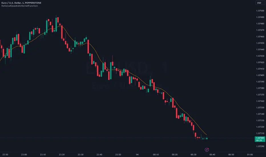
RationalQuadraticKernelFunctionDescription:
An optimised library for non-repainting Rational Quadratic Kernel Library. Added lookbackperiod and a validation to prevent division by zero.
Thanks to original author jdehorty.
Usage:
1. Import the library into your Pine Script code using the library function.
import vinayakavajiraya/RationalQuadraticKernelFunction/1
2. Call the Main Function:
Use the rationalQuadraticKernel function to calculate the Rational Quadratic Kernel estimate.
Provide the following parameters:
`_src` (series float): The input series of float values, typically representing price data.
`_lookback` (simple int): The lookback period for the kernel calculation (an integer).
`_relativeWeight` (simple float): The relative weight factor for the kernel (a float).
`startAtBar` (simple int): The bar index to start the calculation from (an integer).
rationalQuadraticEstimate = rationalQuadraticKernel(_src, _lookback, _relativeWeight, startAtBar)
3. Plot the Estimate:
Plot the resulting estimate on your TradingView chart using the plot function.
plot(rationalQuadraticEstimate, color = color.red, title = "Rational Quadratic Kernel Estimate")
Parameter Explanation:
`_src`: The input series of price data, such as 'close' or any other relevant data.
`_lookback`: The number of previous bars to consider when calculating the estimate. Higher values capture longer-term trends.
`_relativeWeight`: A factor that controls the importance of each data point in the calculation. A higher value emphasizes recent data.
`startAtBar`: The bar index from which the calculation begins.
Example Usage:
Here's an example of how to use the library to calculate and plot the Rational Quadratic Kernel estimate for the 'close' price series:
//@version=5
library("RationalQuadraticKernelFunctions", true)
rationalQuadraticEstimate = rationalQuadraticKernel(close, 11, 1, 24)
plot(rationalQuadraticEstimate, color = color.orange, title = "Rational Quadratic Kernel Estimate")
This example calculates the estimate for the 'close' price series, considers the previous 11 bars, assigns equal weight to all data points, and starts the calculation from the 24th bar. The result is plotted as an orange line on the chart.
Highly recommend to customize the parameters to suit your analysis needs and adapt the library to your trading strategies.
MOST + Moving Average ScreenerScreener version of Anıl Özekşi's Moving Stop Loss (MOST) Indicator:
USERS MAY SCREEN MOST WITH 11 DIFFERENT TYPES OF MOVING AVERAGES + THEY CAN ALSO SCREEN SIGNALS WITH THAT 11 MOVING AVERAGES INSTEAD OF USING MOST LINE.
Adjustable Moving Average Types:
SMA : Simple Moving Average
EMA : Exponential Moving Average
WMA : Weighted Moving Average
DEMA : Double Exponential Moving Average
TMA : Triangular Moving Average
VAR : Variable Index Dynamic Moving Average aka VIDYA
WWMA : Welles Wilder's Moving Average
ZLEMA : Zero Lag Exponential Moving Average
TSF : True Strength Force
HULL : Hull Moving Average
TILL : Tillson T3 Moving Average
About Screener Panel:
Users can explore 20 different and user-defined tickers, which can be changed from the SETTINGS (shares, crypto, commodities...) on this screener version.
The screener panel shows up right after the bars on the right side of the chart.
-In this screener version of MOST, users can define the number of demanded tickers (symbols) from 1 to 20 by checking the relevant boxes on the settings tab.
-All selected tickers can be screened in different timeframes.
-Also, different timeframes of the same Ticker can be screened.
IMPORTANT NOTICE:
Screener shows the results in 3 different logic:
1st LOGIC (Default Settings):
BUY AND SELL SIGNALS of MOST and MOVING AVERAGE LINE
Most Buy Signal: Moving Average Crosses ABOVE the MOST LINE
Most Sel Signal: Moving Average Crosses BELOW the MOST LINE
Tickers seen in green are the ones that are in an uptrend, according to MOST.
The ones that appear in red are those in the SELL signal, in a downtrend.
The numbers before each Ticker indicate how many bars passed after MOST's last BUY or SELL signal.
For example, according to the indicator, when BTCUSDT appears (3) in GREEN, Bitcoin switched to a BUY signal 3 bars ago.
2nd LOGIC (Moving Average & Price Flips Screener Mode):
This mode can only be activated by checking the 'Activate Moving Average Screening Mode' box on the settings menu.
MOST line will be disappeared after checking the box.
Buy Signal: When the Selected Price crosses ABOVE the selected Moving Average.
Sell Signal: When the Selected Price crosses BELOW the selected Moving Average.
Tickers seen in green are the ones that are in an uptrend, according to Moving Average & Price Flips.
The ones that appear in red are those in the SELL signal, in a downtrend.
The numbers before each Ticker indicate how many bars passed after the last BUY or SELL signal of Moving Average & Price Flips.
For example, according to the indicator, when BTCUSDT appears (3) in GREEN, Bitcoin switched to a BUY signal 3 bars ago.
3rd LOGIC (Moving Average Color Change Screener Mode):
Both 'Activate Moving Average Screening Mode' and 'Activate Moving Average Color Change Screening Mode' boxes must be checked in the settings tab.
Moving Average Line will turn out into two colors.
Green color means the moving average value is greater than the previous bar's value.
Red color means the moving average value is smaller than the previous bar's value.
Buy Signal: After the Selected Moving Average turns GREEN from red.
Sell Signal: After the Selected Moving Average turns RED from green.
-Screener shows the information about the color changes of the selected Moving Average with default settings.
If this option is preferred, users are advised to enlarge the length to have better signals.
Tickers seen in green are the ones that are in an uptrend, according to Moving Average Color.
The ones that appear in red are those in the SELL signal, in a downtrend.
The numbers before each Ticker indicate how many bars passed after the last BUY or SELL signal of Moving Average Color Change.
For example, according to the indicator, when BTCUSDT appears (3) in GREEN, Bitcoin switched to a BUY signal 3 bars ago.

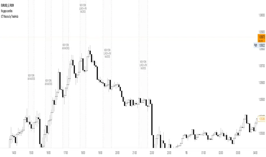
ICT Macros [LuxAlgo]The ICT Macros indicator aims to highlight & classify ICT Macros, which are time intervals where algorithmic trading takes place to interact with existing liquidity or to create new liquidity.
🔶 SETTINGS
🔹 Macros
Macro Time options (such as '09:50 AM 10:10'): Enable specific macro display.
Top Line , Mid Line , Bottom Line and Extending Lines options: Controls the lines for the specific macro.
🔹 Macro Classification
Length : A length to detect Market Structure Brakes and classify macro type based on detection.
Swing Area : Swing or Liquidity Area selection, highest/lowest of the wick or the candle bodies.
Accumulation , Manipulation and Expansion color options for the classified macros.
🔹 Others
Macro Texts : Controls both the size and the visibility of the macro text.
Alert Macro Times in Advance (Minutes) : This option will plot a vertical line presenting the start of the next macro time. The line will not appear all the time, but it will be there based on remaining minutes specified in the option.
Daylight Saving Time (DST) : Adjust time appropriate to Daylight Saving Time of the specific region.
🔶 USAGE
A macro is a way to automate a task or procedure which you perform on a regular basis.
In the context of ICT's teachings, a macro is a small program or set of instructions that unfolds within an algorithm, which influences price movements in the market. These macros operate at specific times and can be related to price runs from one level to another or certain market behaviors during specific time intervals. They help traders anticipate market movements and potential setups during specific time intervals.
To trade these effectively, it is important to understand the time of day when certain macros come into play, and it is strongly advised to introduce the concept of liquidity in your analysis.
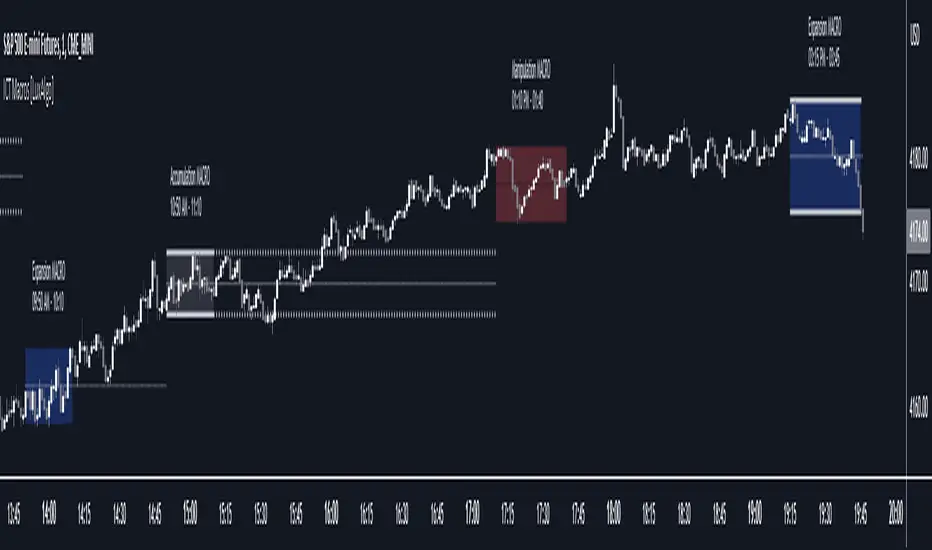
Macros can be classified into three categories where the Macro classification is calculated based on the Market Structure prior to macro and the Market Structure during the macro duration:
Manipulation Macro
Manipulation macros are characterized by liquidity being swept both on the buyside and sellside.
Expansion Macro
Expansion macros are characterized by liquidity being swept only on the buyside or sellside. Prices within these macros are highly correlated with the overall trend.
Accumulation Macro
Accumulation macros are characterized by an accumulation of liquidity. Prices within these macros tend to range.
The script returns the maximum/minimum price values reached during the macro interval alongside the average between the maximum/minimum and extends them until a new macro starts. These levels can act as supports and resistances.
🔶 DETAILS
All required data for the macro detection and classification is retrieved using 1 minute data sets, this includes candles as well as pivot/swing highs and lows. This approach guarantees the visually presented objects are same (same highs/lows) on higher timeframes as well as the macro classification remain same as it is in 1 min charts.
8 Macros can be displayed by the script (4 are enabled by default):
02:33 AM 03:00 London Macro
04:03 AM 04:30 London Macro
08:50 AM 09:10 New York Macro
09:50 AM 10:10 New York Macro
10:50 AM 11:10 New York Macro
11:50 AM 12:10 New York Launch Macro
13:10 PM 13:40 New York Macro
15:15 PM 15:45 New York Macro
🔶 ALERTS
When an alert is configured, the user will have the ability to be notified in advance of the next Macro time, where the value specified in 'Alert Macro Times in Advance (Minutes)' option indicates how early to be notified.
🔶 LIMITATIONS
The script is supported on 1 min, 3 mins and 5 mins charts.
🔶 RELATED SCRIPTS
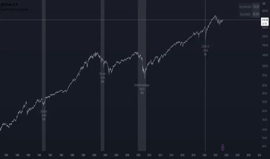
Recessions & crises shading (custom dates & stats)Shades your chart background to flag events such as crises or recessions, in similar fashion to what you see on FRED charts. The advantage of this indicator over others is that you can quickly input custom event dates as text in the menu to analyse their impact for your specific symbol. The script automatically labels, calculates and displays the peak to through percentage corrections on your current chart.
By default the indicator is configured to show the last 6 US recessions. If you have custom events which will benefit others, just paste the input string in the comments below so one can simply copy/paste in their indicator.
Example event input (No spaces allowed except for the label name. Enter dates as YYYY-MM-DD.)
2020-02-01,2020-03-31,COVID-19
2007-12-01,2009-05-31,Subprime mortgages
2001-03-01,2001-10-30,Dot-com bubble
1990-07-01,1991-03-01,Oil shock
1981-07-01,1982-11-01,US unemployment
1980-01-01,1980-07-01,Volker
1973-11-01,1975-03-01,OPEC
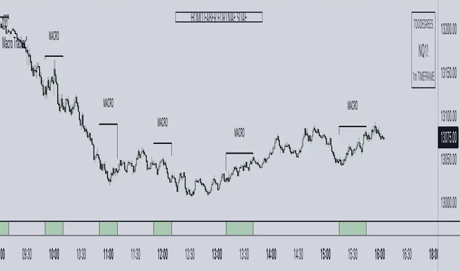
ICT Algorithmic Macro Tracker° (Open-Source) by toodegreesDescription:
The ICT Algorithmic Macro Tracker° Indicator is a powerful tool designed to enhance your trading experience by clearly and efficiently plotting the known ICT Macro Times on your chart.
Based on the teachings of the Inner Circle Trader , these Time windows correspond to periods when the Interbank Price Delivery Algorithm undergoes a series of checks ( Macros ) and is probable to move towards Liquidity.
The indicator allows traders to visualize and analyze these crucial moments in NY Time:
- 2:33-3:00
- 4:03-4:30
- 8:50-9:10
- 9:50-10:10
- 10:50-11:10
- 11:50-12:10
- 13:10-13:50
- 15:15-15:45
By providing a clean and clutter-free representation of ICT Macros, this indicator empowers traders to make more informed decisions, optimize and build their strategies based on Time.
Massive shoutout to @reastruth for his ICT Macros Indicator , and for allowing to create one of my own, go check him out!
Indicator Features:
– Track ongoing ICT Macros to aid your Live analysis.
- Gain valuable insights by hovering over the plotted ICT Macros to reveal tooltips with interval information.
– Plot the ICT Macros in one of two ways:
"On Chart": visualize ICT Macro timeframes directly on your chart, with automatic adjustments as Price moves.
Pro Tip: toggle Projections to see exactly where Macros begin and end without difficulty.
"New Pane": move the indicator two a New Pane to see both Live and Upcoming Macro events with ease in a dedicated section
Pro Tip: this section can be collapsed by double-clicking on the main chart, allowing for seamless trading preparation.
This indicator is available only on the TradingView platform.
⚠️ Open Source ⚠️
Coders and TV users are authorized to copy this code base, but a paid distribution is prohibited. A mention to the original author is expected, and appreciated.
⚠️ Terms and Conditions ⚠️
This financial tool is for educational purposes only and not financial advice. Users assume responsibility for decisions made based on the tool's information. Past performance doesn't guarantee future results. By using this tool, users agree to these terms.
ICT Macros by CryptoforICT Macros by Cryptofor
Time periods in which the price is most volatile. At this time, the algorithm is programmed to attack liquidity or fill a significant FVG from which the OF can continue.
Plots of macros:
1. London Macros:
02:33 - 03:00
04:03 - 04:30
2. New York AM Macros:
08:50 - 09:10
09:50 - 10:10
10:50 - 11:10
3. New York Lunch + PM Macros:
11:50 - 12:10
13:10 - 13:40
15:15 - 15:45
Features:
Flexible line settings
Flexible text settings
Display data for all time or for the last 24 hours
Switch for each type of macro
Macro background color settings