OPEN-SOURCE SCRIPT
Ehlers Phasor Analysis (PHASOR)
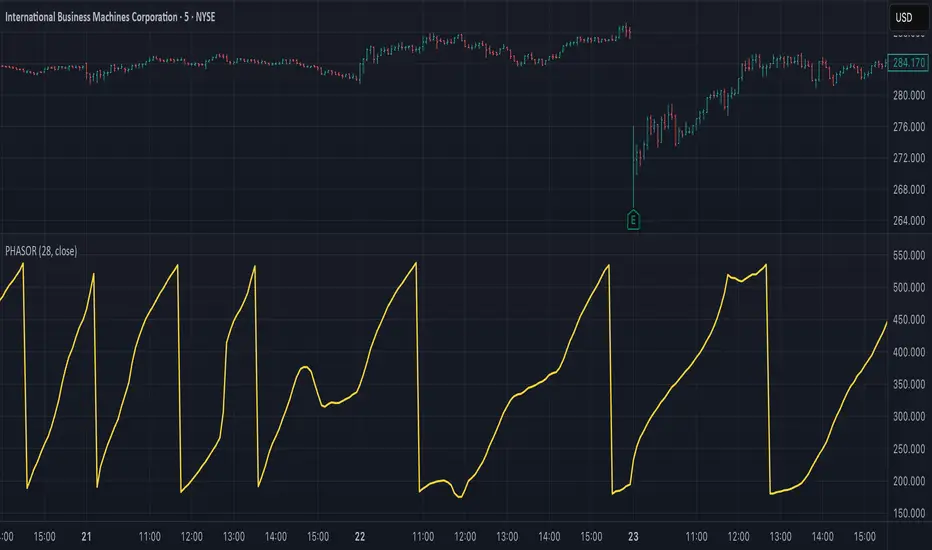
# PHASOR: Phasor Analysis (Ehlers)
## Overview and Purpose
The Phasor Analysis indicator, developed by John Ehlers, represents an advanced cycle analysis tool that identifies the phase of the dominant cycle component in a time series through complex signal processing techniques. This sophisticated indicator uses correlation-based methods to determine the real and imaginary components of the signal, converting them to a continuous phase angle that reveals market cycle progression. Unlike traditional oscillators, the Phasor provides unwrapped phase measurements that accumulate continuously, offering unique insights into market timing and cycle behavior.
## Core Concepts
* **Complex Signal Analysis** — Uses real and imaginary components to determine cycle phase
* **Correlation-Based Detection** — Employs Ehlers' correlation method for robust phase estimation
* **Unwrapped Phase Tracking** — Provides continuous phase accumulation without discontinuities
* **Anti-Regression Logic** — Prevents phase angle from moving backward under specific conditions
Market Applications:
* **Cycle Timing** — Precise identification of cycle peaks and troughs
* **Market Regime Analysis** — Distinguishes between trending and cycling market conditions
* **Turning Point Detection** — Advanced warning system for potential market reversals
## Common Settings and Parameters
| Parameter | Default | Function | When to Adjust |
|-----------|---------|----------|----------------|
| Period | 28 | Fixed cycle period for correlation analysis | Match to expected dominant cycle length |
| Source | Close | Price series for phase calculation | Use typical price or other smoothed series |
| Show Derived Period | false | Display calculated period from phase rate | Enable for adaptive period analysis |
| Show Trend State | false | Display trend/cycle state variable | Enable for regime identification |
## Calculation and Mathematical Foundation
**Technical Formula:**
**Stage 1: Correlation Analysis**
For period $n$ and source $x_t$:
Real component correlation with cosine wave:
$$R = \frac{n \sum x_t \cos\left(\frac{2\pi t}{n}\right) - \sum x_t \sum \cos\left(\frac{2\pi t}{n}\right)}{\sqrt{D_{cos}}}$$
Imaginary component correlation with negative sine wave:
$$I = \frac{n \sum x_t \left(-\sin\left(\frac{2\pi t}{n}\right)\right) - \sum x_t \sum \left(-\sin\left(\frac{2\pi t}{n}\right)\right)}{\sqrt{D_{sin}}}$$
where $D_{cos}$ and $D_{sin}$ are normalization denominators.
**Stage 2: Phase Angle Conversion**
$$\theta_{raw} = \begin{cases}
90° - \arctan\left(\frac{I}{R}\right) \cdot \frac{180°}{\pi} & \text{if } R \neq 0 \\
0° & \text{if } R = 0, I > 0 \\
180° & \text{if } R = 0, I \leq 0
\end{cases}$$
**Stage 3: Phase Unwrapping**
$$\theta_{unwrapped}(t) = \theta_{unwrapped}(t-1) + \Delta\theta$$
where $\Delta\theta$ is the normalized phase difference.
**Stage 4: Ehlers' Anti-Regression Condition**
$$\theta_{final}(t) = \begin{cases}
\theta_{final}(t-1) & \text{if regression conditions met} \\
\theta_{unwrapped}(t) & \text{otherwise}
\end{cases}$$
**Derived Calculations:**
Derived Period: $P_{derived} = \frac{360°}{\Delta\theta_{final}}$ (clamped to [1, 60])
Trend State:
$$S_{trend} = \begin{cases}
1 & \text{if } \Delta\theta \leq 6° \text{ and } |\theta| \geq 90° \\
-1 & \text{if } \Delta\theta \leq 6° \text{ and } |\theta| < 90° \\
0 & \text{if } \Delta\theta > 6°
\end{cases}$$
> 🔍 **Technical Note:** The correlation-based approach provides robust phase estimation even in noisy market conditions, while the unwrapping mechanism ensures continuous phase tracking across cycle boundaries.
## Interpretation Details
* **Phasor Angle (Primary Output):**
- **+90°**: Potential cycle peak region
- **0°**: Mid-cycle ascending phase
- **-90°**: Potential cycle trough region
- **±180°**: Mid-cycle descending phase
* **Phase Progression:**
- Continuous upward movement → Normal cycle progression
- Phase stalling → Potential cycle extension or trend development
- Rapid phase changes → Cycle compression or volatility spike
* **Derived Period Analysis:**
- Period < 10 → High-frequency cycle dominance
- Period 15-40 → Typical swing trading cycles
- Period > 50 → Trending market conditions
* **Trend State Variable:**
- **+1**: Long trend conditions (slow phase change in extreme zones)
- **-1**: Short trend or consolidation (slow phase change in neutral zones)
- **0**: Active cycling (normal phase change rate)
## Applications
* **Cycle-Based Trading:**
- Enter long positions near -90° crossings (cycle troughs)
- Enter short positions near +90° crossings (cycle peaks)
- Exit positions during mid-cycle phases (0°, ±180°)
* **Market Timing:**
- Use phase acceleration for early trend detection
- Monitor derived period for cycle length changes
- Combine with trend state for regime-appropriate strategies
* **Risk Management:**
- Adjust position sizes based on cycle clarity (derived period stability)
- Implement different risk parameters for trending vs. cycling regimes
- Use phase velocity for stop-loss placement timing
## Limitations and Considerations
* **Parameter Sensitivity:**
- Fixed period assumption may not match actual market cycles
- Requires cycle period optimization for different markets and timeframes
- Performance degrades when multiple cycles interfere
* **Computational Complexity:**
- Correlation calculations over full period windows
- Multiple mathematical transformations increase processing requirements
- Real-time implementation requires efficient algorithms
* **Market Conditions:**
- Most effective in markets with clear cyclical behavior
- May provide false signals during strong trending periods
- Requires sufficient historical data for correlation analysis
Complementary Indicators:
* MESA Adaptive Moving Average (cycle-based smoothing)
* Dominant Cycle Period indicators
* Detrended Price Oscillator (cycle identification)
## References
1. Ehlers, J.F. "Cycle Analytics for Traders." Wiley, 2013.
2. Ehlers, J.F. "Cybernetic Analysis for Stocks and Futures." Wiley, 2004.
オープンソーススクリプト
TradingViewの精神に則り、このスクリプトの作者はコードをオープンソースとして公開してくれました。トレーダーが内容を確認・検証できるようにという配慮です。作者に拍手を送りましょう!無料で利用できますが、コードの再公開はハウスルールに従う必要があります。
github.com/mihakralj/pinescript
A collection of mathematically rigorous technical indicators for Pine Script 6, featuring defensible math, optimized implementations, proper state initialization, and O(1) constant time efficiency where possible.
A collection of mathematically rigorous technical indicators for Pine Script 6, featuring defensible math, optimized implementations, proper state initialization, and O(1) constant time efficiency where possible.
免責事項
この情報および投稿は、TradingViewが提供または推奨する金融、投資、トレード、その他のアドバイスや推奨を意図するものではなく、それらを構成するものでもありません。詳細は利用規約をご覧ください。