Smart Trader,Episode 1, by Ata Sabanci | Unified Matrix⚠️ **CRITICAL: READ BEFORE USING** ⚠️
This strategy is **100% VOLUME-BASED** and requires **Lower Timeframe (LTF) intrabar data** for accurate calculations. Please understand the following limitations before using:
**📊 DATA ACCURACY LEVELS:**
• **1T (Tick)** — Most accurate, real volume distribution per tick
• **1S (1 Second)** — Reasonably accurate approximation
• **15S (15 Seconds)** — Good approximation, longer historical data available
• **1M (1 Minute)** — Rough approximation, maximum historical data range
**⚠️ BACKTEST & REPLAY LIMITATIONS:**
• TradingView's Strategy Tester uses historical LTF data which may be limited depending on your subscription plan
• Replay mode results may differ from live trading due to data availability
• For longer backtest periods, use higher LTF settings (15S or 1M)
• Not all symbols/exchanges support tick-level data
• Crypto and Forex typically have better LTF data availability than stocks
**💡 A NOTE ON TOOLS:**
Successful trading requires proper tools. Higher TradingView plans provide access to more historical intrabar data, which directly impacts the accuracy of volume-based calculations. More precise volume data leads to more reliable signals. Consider this when evaluating your trading infrastructure.
**WHY "EPISODE 1"?**
This strategy is titled "Episode 1" because it focuses exclusively on **Highest Buyers (HB)** — a single but powerful concept in volume analysis.
**The Philosophy:**
A single high-volume buying event can tell us a story about market psychology:
• Where did the biggest buyers enter?
• How much of their power remains?
• Are sellers consuming their advantage?
• At what rate is the balance shifting?
By focusing on just ONE aspect of volume analysis, traders can deeply understand how a buying surge affects future price action before moving to more complex multi-factor analysis.
**The Reality:**
This script alone is approximately **2000 lines of code** — and it only analyzes buyers. A comprehensive system covering all aspects (sellers, combined analysis, multi-timeframe correlation) would be significantly larger and computationally heavier. Breaking this into focused modules allows for:
• Deeper understanding of each component
• Lighter, more responsive scripts
• Educational progression from simple to complex
**OVERVIEW**
Smart Trader EP1 is a volume-based trading strategy that tracks the balance of power between buyers and sellers through the lens of the **Highest Buyers event**. Unlike traditional indicators that rely on price patterns or mathematical formulas, this strategy analyzes *actual volume flow* to identify who is in control of the market.
The core philosophy is simple: **markets move when one side (buyers or sellers) exhausts their power while the opposing side accumulates strength.** By measuring this power shift in real-time, the strategy identifies high-probability entry and exit points.
**HOW IT WORKS**
**1. Volume Engine**
The strategy splits each candle's volume into buying volume and selling volume using intrabar data. In *Intrabar (Precise)* mode, it uses actual tick-by-tick or second-by-second data to calculate the exact buy/sell distribution. In *Geometry* mode, it approximates based on candle structure (close position within the range).
**2. Event Detection**
Within the lookback window, the strategy identifies key events:
• **HB (Highest Buyers)** — The candle with maximum buying volume (potential resistance when exhausted)
• **HS (Highest Sellers)** — The candle with maximum selling volume (potential support when exhausted)
• **LB (Lowest Buyers)** — The candle with minimum buying volume (buyer absence)
• **LS (Lowest Sellers)** — The candle with minimum selling volume (seller absence)
These events create dynamic support and resistance levels based on actual volume, not arbitrary price levels.
**3. Power Tracking (Attrition Model)**
For the Highest Buyers event (HB), the strategy tracks:
• **Start Power (X)** — The initial buying volume at the HB event
• **Consumed Power (Y)** — How much selling volume has accumulated since the event
• **Remaining Power (Z)** — Start Power minus Consumed Power (X - Y)
• **Opponent Dominance** — When Remaining Power goes negative (Z < 0), sellers have overtaken buyers
Think of it like a battle: buyers establish a position (HB), and sellers gradually consume their power. When buyers' power is exhausted (Remaining Power ≤ 0), sellers have taken control.
**4. Depletion Markers**
Visual markers appear on the chart when power reaches critical thresholds:
• **🔋** — Buyers consumed 100% (Remaining = 0)
• **🚨** — Buyers consumed 200% (Opponent Dominance = 100%)
• **🪫** — Sellers consumed 100%
• **⚠️** — Sellers consumed 200%
**5. Cumulative Delta**
Beyond tracking power at specific events, the strategy calculates the cumulative buy volume minus sell volume since the HB event. This shows the *net flow* of money:
• **Positive Delta** — More buying than selling since HB (bullish pressure)
• **Negative Delta** — More selling than buying since HB (bearish pressure)
**6. Trend Channel**
A 5-point linear regression channel identifies the current trend:
• **UPTREND** — Both upper and lower channel lines slope upward
• **DOWNTREND** — Both lines slope downward
• **RANGING** — Mixed or flat slopes
The strategy also tracks where the HB event occurred within this channel (TOP, UPPER, MIDDLE, LOWER, BOTTOM) to contextualize the signal.
**7. Nearest Event Analysis**
The strategy identifies which event is closest to the current candle and analyzes the price action *after* that event:
• How many bullish vs bearish candles followed?
• Does post-event momentum confirm or contradict the event type?
This prevents false signals when, for example, a bearish event occurs but is immediately followed by strong bullish candles.
**SIGNAL LOGIC**
**🟢 LONG Signal Conditions:**
• Uptrend with positive cumulative delta and buyers accumulating
• At channel bottom/lower with strong buyer power remaining
• After a bearish event (HS) with bullish post-event momentum (reversal signal)
• Ranging market with positive delta and strong power
**🔴 SHORT Signal Conditions:**
• Downtrend with negative cumulative delta and sellers in control
• Opponent Dominance (buyer power exhausted) with bearish momentum
• Buyer Trap: HB at TOP in uptrend but power exhausted and delta negative
• After a bullish event (HB) with bearish post-event momentum (trap signal)
**⏳ NO_TRADE Conditions:**
• Conflicting signals (e.g., bearish event but bullish post-momentum)
• Ranging market without clear direction
• Mixed power readings
• Price position contradicts signal direction
**STRATEGY EXECUTION**
**Entry Rules:**
• Enter LONG when signal is "LONG" and conditions are valid
• Enter SHORT when signal is "SHORT" and conditions are valid
• **Pyramid**: Up to 2 entries allowed in the same direction (configurable)
• Each entry uses 10% of equity by default
• Only one entry per confirmed candle (prevents multiple fills)
**Stop Loss (Event Line Based):**
• **LONG positions**: Stop Loss placed below the HS line (seller support level)
• **SHORT positions**: Stop Loss placed above the HB line (buyer resistance level)
• A small buffer percentage is added to prevent premature stops
**Take Profit (Event Line Based):**
• **LONG positions**: Take Profit near the HB line (buyer resistance target)
• **SHORT positions**: Take Profit near the HS line (seller support target)
• A small buffer percentage ensures realistic fill expectations
**Exit Rules:**
• Exit LONG when signal changes to SHORT
• Exit SHORT when signal changes to LONG
• **NO_TRADE signal = HOLD** (do not exit, wait for clear direction)
• SL/TP orders remain active regardless of signal changes
**SETTINGS GUIDE**
**⚙️ General Settings:**
• *Calculation Method* — Choose between Intrabar (Precise) or Geometry (approximation)
• *Intrabar Resolution* — LTF for volume data (1T, 1S, 15S, 1M)
• *Lookback Length* — Window for scanning events (10-150 bars)
• *Timezone Offset* — Adjust clock display to your local time
**📊 Matrix Display Settings:**
• *Show Unified Matrix* — Toggle the information dashboard
• *Show Event Lines* — Toggle horizontal lines at event prices
• *Panel Size/Position* — Customize dashboard appearance
• *Projection Bars* — Extend event lines into the future
• *Depletion Threshold* — Percentage for depletion markers (default: 100%)
**🏷️ Rank Labels Settings:**
• *Show Rank Labels (HB/HS)* — Display labels on highest volume candles
• *Show Low Labels (LB/LS)* — Display labels on lowest volume candles
• *Ranks Count* — Number of rankings to display (1-5)
**📐 Trend Channel Settings:**
• *Show Trend Channel* — Toggle the 5-point regression channel
• *Line Color/Fill/Width/Style* — Customize channel appearance
**🎯 Trade Signal Settings:**
• *Long: Min Remaining Power %* — Minimum buyer power for LONG signal (default: 50%)
• *Short: Max Remaining Power %* — Maximum power for SHORT signal (default: 30%)
• *Opponent Dominance Threshold* — When to consider power "exhausted" (default: 0%)
• *Max Decay Angle* — Maximum consumption rate for valid entries (default: 60°)
**📈 Strategy Execution Settings:**
• *Enable Strategy* — Turn automatic trading on/off
• *Allow LONG/SHORT* — Enable or disable specific directions
• *Max Pyramid Entries* — Maximum entries in same direction (1-3)
• *SL Buffer %* — Distance below/above event line for stop loss (default: 0.15%)
• *TP Buffer %* — Distance from event line for take profit (default: 0.05%)
**VISUAL ELEMENTS**
**Chart Labels:**
• **#1 HB** — Highest Buyers (rank label on candle high)
• **#1 HS** — Highest Sellers (rank label on candle low)
• **#1 LB** — Lowest Buyers (rank label on candle high)
• **#1 LS** — Lowest Sellers (rank label on candle low)
• **🔋 / 🚨** — Buyer power depletion markers
• **🪫 / ⚠️** — Seller power depletion markers
**Event Lines:**
• **Blue horizontal lines** — HB price levels (buyer entry points)
• **Red horizontal lines** — HS price levels (seller entry points)
• **Cyan lines** — LB price levels
• **Orange lines** — LS price levels
• **Dashed extensions** — Projected levels into future bars
**Trend Channel:**
• **Orange lines** — Upper and lower channel boundaries (5-point regression)
• **Orange fill** — Channel area (90% transparency)
**Matrix Dashboard (6 rows):**
• Row 1: Header with symbol, LTF setting, and local clock
• Row 2: Volume snapshot (Total, Buy, Sell, Delta)
• Row 3: Column headers
• Row 4: Highest Buyers data (Age, Start Power, Consumed, Remaining, Decay, ETA)
• Row 5: Highest Sellers data
• Row 6: Signal Evaluation (Trend, Zone, Nearest Event, Signal, Reason)
**Strategy Markers:**
• **Green triangle up** — LONG entry
• **Red triangle down** — SHORT entry
• **Faded triangles** — Pyramid entries
• **Colored lines** — SL (red) and TP (green) levels when in position
**BEST PRACTICES**
**For Maximum Accuracy:**
1. Use **1T (tick)** or **1S** intrabar resolution when available
2. Trade liquid markets with good volume data (crypto majors, forex majors, high-volume stocks)
3. Use smaller lookback length (20-30) to ensure all bars have valid LTF data
4. Monitor the "Intrabar Valid Bars" counter in the matrix header
5. If you see data warnings, reduce lookback or increase LTF resolution
**For Longer Backtests:**
1. Use **15S or 1M** intrabar resolution for more historical data
2. Increase lookback length if needed
3. Understand that accuracy decreases with higher LTF settings
4. Consider using Geometry mode for very long backtests (approximation but always available)
**Understanding the Signals:**
• Pay attention to the signal *reasoning* shown in the matrix — it explains WHY
• **NO_TRADE** means the system sees conflicting factors — respect this caution
• Event lines act as dynamic S/R — they update as new volume events occur
• Cumulative Delta (Δ) often provides early warning of trend changes
**Risk Management:**
• The default 10% per entry with max 2 pyramids = 20% maximum exposure
• Event-line-based SL/TP provides logical levels based on actual volume events
• Always verify signals with your own analysis before trading
**INTERPRETING THE MATRIX**
**Power Status Examples:**
• *Remaining Power: 75%* — Buyers still have most of their strength
• *Remaining Power: 25%* — Buyers nearly exhausted, watch for reversal
• *Opponent Dominance: -50%* — Sellers have consumed 150% of buyer power (strong bearish)
**Decay Angle:**
• *Low angle (0-30°)* — Slow consumption, power lasting longer
• *High angle (60-90°)* — Rapid consumption, expect quick exhaustion
**ETA to Parity:**
• Shows estimated bars until Remaining Power reaches zero
• *"Overtaken"* with 🚨 means sellers have already dominated
**LIMITATIONS & DISCLAIMER**
**Technical Limitations:**
• Requires sufficient historical LTF data (varies by TradingView plan and symbol)
• Intrabar (Precise) mode may show invalid data warnings on symbols with limited history
• Strategy tester may not have access to the same LTF data as live trading
• Maximum 500 lines and 500 labels (TradingView platform limits)
**Important Notes:**
• This strategy focuses on **Highest Buyers only** — it does not analyze all market factors
• Past performance does not guarantee future results
• Volume data quality varies significantly between symbols and exchanges
• The strategy's signals are analytical tools, not trading recommendations
**Risk Disclaimer:**
This strategy is provided for **educational and informational purposes only**. Trading involves substantial risk of loss and is not suitable for all investors.
• Always use proper risk management
• Never risk more than you can afford to lose
• Backtest results may differ significantly from live trading
• You are solely responsible for your trading decisions
**TECHNICAL SPECIFICATIONS**
• Pine Script Version: 6
• Calculation: calc_on_every_tick=true, use_bar_magnifier=true
• Default Capital: 10,000
• Default Position Size: 10% of equity
• Maximum Lines: 500
• Maximum Labels: 500
• External Library: TradingView/ta/10 (for requestUpAndDownVolume)
*Smart Trader EP1 — Understanding Volume, One Event at a Time*
Forecastingtechniques

MTF Probability Predictor v1 (Directional + Market State)This indicator is designed to generate high-confidence market bias by combining price action, chart structure, momentum, divergence analysis, ATR, and VWAP-based volatility assessment.
Instead of providing binary signals, the indicator presents a probability-based decision framework, displaying BUY / SELL confidence percentages in real time. This allows traders to assess signal quality, market strength, and trade suitability before taking a position.

MTF Probability Predictor PRO v2This indicator is designed to generate high-confidence market bias by combining price action, chart structure, momentum, divergence analysis, ATR, and VWAP-based volatility assessment.
Instead of providing binary signals, the indicator presents a probability-based decision framework, displaying BUY / SELL / NEUTRAL confidence percentages in real time. This allows traders to assess signal quality, market strength, and trade suitability before taking a position.
BUY Bias (Trade-Favorable Condition)
A BUY setup is considered favorable when: BUY confidence exceeds 65% AND SELL confidence remains below 10% AND NEUTRAL confidence is 25% or lower
==>> This combination indicates strong directional momentum with minimal opposing pressure, suggesting a higher-probability bullish environment.
SELL Bias (Trade-Favorable Condition)
A SELL setup is considered favorable when: SELL confidence exceeds 65% AND BUY confidence remains below 10% AND NEUTRAL confidence is 25% or lower
==>> This reflects dominant bearish control, reduced market indecision, and a clearer downside directional bias.
NEUTRAL Bias (No-Trade Zone)
A NEUTRAL condition is identified when: NEUTRAL confidence rises above 50% or higher
==>> This indicates range-bound or transitional market behavior, where directional conviction is weak. During such conditions, it is recommended to avoid trading and allow the market to establish a clearer trend.
Key Benefits -
Probability-driven signal clarity
Reduced false signals in sideways markets
Suitable for scalping, intraday, and swing trading
Designed to support disciplined, rules-based decision making

Smart Money Concept, Modern ViewSmart Money Concept, Modern View (SMCMV)
Institutional Volume Flow Analysis with VWMA Matrix
━━━━━━━━━━━━━━━━━━━━━━━━━━━━━━━━━━━━━━━━━━━━━━━━━━
📌 OVERVIEW
SMCMV is an advanced institutional-grade indicator that combines Volume-Weighted Moving Average (VWMA) matrix analysis with sophisticated volume decomposition to detect buyer and seller entry points. The indicator provides a comprehensive real-time dashboard displaying market structure, volume dynamics, and validated trading signals.
Key Features:
• Dual Volume Model: Geometry-based (candle range split) and Intrabar (precise LTF data)
• 10-Period VWMA Spectrum: Multi-timeframe support/resistance matrix (7, 13, 19, 23, 31, 41, 47, 67, 83, 97)
• 5-Layer Scoring System: 100-point institutional-grade signal quality assessment
• State Machine Signal Engine: Validated entry/exit signals with timer and range confirmation
• Real-time Prediction Engine: Candle-by-candle buyer/seller probability estimation
• High Volume Node Detection: Automatic identification of significant volume zones
━━━━━━━━━━━━━━━━━━━━━━━━━━━━━━━━━━━━━━━━━━━━━━━━━━
📊 DASHBOARD REFERENCE
1) NOW VECTOR (Current Market State)
This section captures the immediate market conditions:
• FLOW ANGLE: Directional angle of price movement in degrees (from VWMA-5). Positive = bullish, Negative = bearish.
• LTP: Last Traded Price - current close price.
• NET FLOW (Δ): Volume Delta - net difference between buying and selling volume. Shows ⚡+ or ⚡-.
• LIQUIDITY: Total volume on the current bar (K/M format).
• BUY VOL: Estimated buying volume based on selected model.
• SELL VOL: Estimated selling volume.
• BID PRES.: Buying volume as percentage of total volume.
• ASK PRES.: Selling volume as percentage of total volume.
• DIRECTION: Current state with hysteresis: BULL (🐂), BEAR (🐻), or NEUT (⚪).
2) DATA QUALITY / CONFIG
Configuration status and data integrity monitoring:
• VOL MODEL: INTRABAR (uses LTF data) or GEOMETRY (estimates from candle structure).
• IB LTF: Intrabar Lower Timeframe for precise volume decomposition.
• MODE: Micro (7 periods: 7-47) or Macro (10 periods: 7-97).
• IB OK: Intrabar data validity - OK or NO.
• IB STREAK: Consecutive bars with valid intrabar data.
• LATENCY: Data freshness indicator. ✓ = current, ↺ = using historical reference.
3) STRUCTURE RADAR
Market structure analysis showing price position relative to VWMA matrix:
• WIRES ▲/▼: Count of VWMAs above (resistance) and below (support).
• RES: Nearest Resistance - shows MA period, "ZN RES", or "BLUE SKY".
• SUPP: Nearest Support - shows MA period, "ZN SUPP", or "FREE FALL".
4) ACTIVE INTERACTION
Real-time analysis of price interaction with key levels:
• Header Status: "⚠ TESTING SUPPLY (ASK SIDE)" / "⚠ TESTING DEMAND (BID SIDE)" / "--- NO KEY INTERACTION ---"
• TARGET: Active level being tested (MA period or zone type).
• TEST LEVEL: Exact price level being tested.
• SCORE: Total score (0-100%) with letter grade .
• VOLUME POWER: Volume ratio vs historical average (e.g., "2.5x").
• BREAKOUT: "CONFIRMED" if attacking volume exceeds defending, "REJECTED" otherwise.
• DELTA DIR: "ALIGNED" if delta matches accumulation trend, "CONFLICT" if opposing.
━━━━━━━━━━━━━━━━━━━━━━━━━━━━━━━━━━━━━━━━━━━━━━━━━━
🎯 5-LAYER SCORING SYSTEM (100 Points Total)
Layer 1: Volume Quality (Max 25 pts)
• Mass (0-10): Volume ratio vs average. 0.5x=0, 1.0x=5, 2.0x=8, 3.0x+=10
• Spike (0-8): Volume Z-Score intensity
• Trend (0-7): Volume trend alignment with price direction
Layer 2: Battle Structure (Max 25 pts)
• Break (0-10): Breakout intensity ratio (attacker vs defender)
• Dom (0-8): Internal dominance ratio
• Pres (0-7): Pressure imbalance percentage
Layer 3: Flow & Energy (Max 20 pts)
• Delta (0-8): Delta alignment with accumulation trend
• Accel (0-6): Delta acceleration
• Mom (0-6): Flow momentum
Layer 4: Geometry (Max 15 pts)
• Impact (0-7): Impact angle directness
• Vec (0-5): Vector alignment
• PriceZ (0-3): Price Z-Score position
Layer 5: Army Structure (Max 15 pts)
• Stack (0-5): MA stack depth
• Conf (0-5): Confluence percentage
• Trend (0-5): Trend alignment count (7>13, 13>23, 23>97)
Grade Scale:
• A+ = 90-100 pts (Exceptional)
• A = 80-89 pts (Strong)
• B+ = 70-79 pts (Good)
• B = 60-69 pts (Moderate)
• C+ = 50-59 pts (Below average)
• C/D/F = Below 50 pts (Weak)
━━━━━━━━━━━━━━━━━━━━━━━━━━━━━━━━━━━━━━━━━━━━━━━━━━
5) SIGNAL STATUS PANEL
Real-time signal state machine status:
• Header: "🐂 BUYERS ACTIVE" / "🐻 SELLERS ACTIVE" / "⏳ VALIDATING..." / "⏸ RANGE / FLAT"
• LOCK PRICE: Price at which signal was locked/confirmed.
• RANGE ±: Validation range percentage.
• POSITION: Price vs lock: "▲ ABOVE" / "▼ BELOW" / "● AT LOCK"
• DISTANCE: Percentage distance from lock price.
• vs RANGE: Position vs validation range: "IN_RANGE" / "ABOVE" / "BELOW"
• VAL TICKS: Validation progress (current/required ticks).
6) REALTIME PREDICTION PANEL
Candle prediction engine:
• WINNER: Predicted dominant side: "BUYERS" / "SELLERS" / "NEUTRAL"
• CONFIDENCE: Prediction confidence percentage.
• ACCURACY: Historical prediction accuracy (session-specific).
• BUY/SELL PROB: Individual probabilities for each side.
━━━━━━━━━━━━━━━━━━━━━━━━━━━━━━━━━━━━━━━━━━━━━━━━━━
🏷️ SIGNAL LABELS REFERENCE
• 🐂 BUYER ENTRY (Green): Confirmed buyer entry signal. Validation complete.
• 🐻 SELLER ENTRY (Red): Confirmed seller entry signal. Validation complete.
• 🔻 REVERSAL BUY→SELL (Magenta): Reversal from buyer to seller position.
• 🔺 REVERSAL SELL→BUY (Cyan): Reversal from seller to buyer position.
• ⏹ EXIT → FLAT (Gray): Position exit to flat/neutral state.
• ⬆ BUYER STRONGER (Small Green): Lock price updated higher during buyer state.
• ⬇ SELLER STRONGER (Small Red): Lock price updated lower during seller state.
Display Modes:
• Minimal: Icon only (hover for tooltip details)
• Normal: Icon + Price level
• Detailed: Full information (price, score, grade)
━━━━━━━━━━━━━━━━━━━━━━━━━━━━━━━━━━━━━━━━━━━━━━━━━━
📈 CHART ELEMENTS
VWMA Spectrum Lines
Colored gradient lines representing the 10-period VWMA matrix. Color progresses from light blue (fast: 7-period) through purple to orange (slow: 97-period). These act as dynamic support/resistance levels weighted by volume.
High Volume Node Lines
• Blue Lines: High Buy Volume zones - potential demand areas
• Red Lines: High Sell Volume zones - potential supply areas
• Yellow Lines: Overlapping zones (buy + sell extremes) - high conflict areas
Lock Price Line & Range Band
• Dashed Line: Locked price level (green for buyers, red for sellers)
• Dotted Lines: Upper/lower bounds of validation range
━━━━━━━━━━━━━━━━━━━━━━━━━━━━━━━━━━━━━━━━━━━━━━━━━━
⚙️ INPUT SETTINGS GUIDE
Volume Model
• Calculation Method: "Geometry (Candle-Range Split)" for universal compatibility or "Intrabar (Precise)" for accurate buy/sell separation.
• Intrabar LTF: Lower timeframe for Intrabar mode (e.g., "1" for 1-minute).
Direction Filter
• Direction Trigger Angle: Threshold for directional state change (default: 1.5°)
• Neutral Reset Angle: Threshold for returning to neutral (default: 0.7°)
Testing Filter
• Level Proximity (%): How close price must be to "test" a level (default: 0.25%)
• Require Wick Touch: If enabled, requires high/low to touch proximity band.
Signal Validation
• Lock Range (%): Price range for validation (default: 0.5%)
• Validation Ticks: Consecutive bars required (default: 3)
• Validation Time: Minimum seconds for real-time confirmation (default: 5)
• Minimum Hold Bars: Stay in position for at least this many bars (default: 5)
• Exit Mode: "Reversal Only" / "Signal Loss" / "Price Stop"
• Stop Loss (%): Exit threshold (default: 1.0%)
Signal Score Filter
• Score Range Minimum: Minimum score for signal generation (default: 10%)
• Score Range Maximum: Maximum score threshold (default: 100%)
━━━━━━━━━━━━━━━━━━━━━━━━━━━━━━━━━━━━━━━━━━━━━━━━━━
💡 USAGE RECOMMENDATIONS
1. Start with Macro mode to see the complete VWMA spectrum, then switch to Micro for cleaner charts.
2. Use Intrabar mode when your broker provides lower timeframe data.
3. Focus on high-grade signals (B+ or better) for higher probability setups.
4. Wait for validation to complete before acting on signals.
5. Use the Lock Price line as your reference for position management.
━━━━━━━━━━━━━━━━━━━━━━━━━━━━━━━━━━━━━━━━━━━━━━━━━━
⚠️ IMPORTANT NOTES
• This indicator is designed for educational and analytical purposes.
• Always combine with proper risk management and additional confirmation.
• Past performance and signal quality do not guarantee future results.
• The prediction accuracy is session-specific and resets on chart reload.
━━━━━━━━━━━━━━━━━━━━━━━━━━━━━━━━━━━━━━━━━━━━━━━━━━
Volume-Based Indicator — Data Granularity & Table Guide
1) Critical warning about data granularity (read first)
Important: This indicator is built entirely on volume-derived calculations (volume, volume delta, and related flow metrics). Because of that, its precision is only as good as the granularity and history of the data you feed it.
The most granular view is a tick-based interval (e.g., 1T = one trade/tick). If tick-based intervals are not available for your symbol or your plan, the closest time-based approximation is a 1-second chart (1S).
If you enable any "high-precision / intrabar" options (anything that relies on the smallest updates), make sure you understand which TradingView plan you are using, because intrabar historical depth (how many bars you can load) varies by plan. More history generally means more stable baselines for volume statistics, regime detection, and long lookback features.
Plan-related notes (TradingView)
TradingView limits how many intrabar historical bars can be loaded, depending on your plan. The exact limits are defined by TradingView and can change over time, but as of the current documentation, the intrabar limits are:
• Basic: 5,000 bars
• Essential: 10,000 bars
• Plus: 10,000 bars
• Premium: 20,000 bars
• Expert: 25,000 bars
• Ultimate: 40,000 bars
Tick charts / tick-based intervals are currently positioned as a feature of professional-tier plans (e.g., Expert/Elite/Ultimate). Availability may also vary by symbol and data feed.

Yearly Projection ExplorerThis indicator helps you understand how the current market period has behaved historically by overlaying the same date window from previous years and projecting it forward from today’s price.
The script works the following way:
Aligns past years to today’s calendar date
Normalizes all paths to the last close at the start
Projects historical performance X bars forward
Displays each year as a separate performance path
Calculates and plots the mean (average) projection for quick reference
🔧 How It Works
Number of Years: choose how many past years to include (e.g. last 10, 20, or 25 years)
Projection Length: choose how many bars (days) ahead to project
Each line shows how the market moved during the same period in a specific year
Labels show the year and total return at the projection end
The mean line highlights the average historical outcome
🧠 Why This Is Useful
Identify seasonal tendencies
Compare current price action to historical analogs
Visualize best / worst historical outcomes
Set realistic expectations for short-term moves
Add context to discretionary or systematic decisions
This tool does not predict the future, but it provides a powerful historical framework to assess what has been typical, rare, or extreme for the current market window.
⚠️ Notes
Script works on timenow variable for now, and you might see unexpected periods if today is a day off.
Results depend on the selected timeframe and instrument
Past performance is not a guarantee of future results
Designed for analysis and context, not standalone signals

Gann Octave Pro - Angles & Time Cycles 🎯 Gann Octave Pro - Angles & Time Cycles
## Complete Gann Trading System - Price, Angles & Time in One Indicator
A professional-grade Gann analysis tool combining **Octave Price Levels**, **Gann Angles (1x1, 2x1, 1x2)**, and **Advanced Time Cycle Projections**. Perfect for traders seeking precision market timing through geometric confluence.
---
## 🌟 Key Features
### 📐 Octave Price Levels
- **5 Key Levels**: 0%, 25%, 50%, 75%, 100%
- **Color-Coded**: Green (support) → Blue (50% pivot) → Red (resistance) → Black (boundaries)
- **Dynamic Updates**: Auto-adjusts to swing structure
- **Trading Edge**: 50% level is the most powerful reversal zone
### 📏 Gann Angles
- **1x1 Angle** (Black) - Natural 45° trend line
- **2x1 Angle** (Red) - Steep acceleration zone
- **1x2 Angle** (Red) - Gradual support/resistance
- **Customizable Extension**: Fixed bars or % of swing length
### ⏰ Advanced Time Cycles
**Three Calculation Methods:**
1. **Angle-Level Confluence** ⭐ (Recommended)
- Calculates intersections of Gann angles with octave levels
- Most sophisticated timing system
- Based on price-time geometry
2. **Swing Duration** - Uses actual swing bar length
3. **Harmonic (Swing/8)** - Classic Gann harmonic division
**Cycle Visualization:**
- **Full Cycles** (Purple, solid) - Major turning points, labeled "◆ FC1 (176 bars) "
- **Sub-Cycles** (Blue, dotted) - Minor pivots, labeled "S1 "
- **Mid-Cycles** (Orange, dashed) - Half-cycle inflection points
- **Past Display**: Shows 4 complete past cycles for validation
- **Future Projection**: Projects 8 future cycles for anticipation
---
## 🎯 How to Use
### Quick Start
1. Apply to chart (works all timeframes/instruments)
2. Select period: Default 44 bars (adjust based on timeframe)
3. Choose cycle method: "Angle-Level Confluence" for best results
4. Observe past cycles to validate timing accuracy
### Trading Strategies
**Triple Confluence Setup** (Highest Probability)
- Price at octave level (especially 50%)
- Price touches Gann angle (1x1 most reliable)
- Time cycle arrives (full cycle preferred)
- **Entry**: On confluence | **Stop**: Below/above octave level | **Target**: Next level
**Cycle Anticipation**
- Enter 1-2 bars before cycle line if price at octave level
- Exit at next cycle or target octave level
- **Edge**: Anticipate cycles instead of reacting
**Angle Breakout + Cycle**
- Price breaks 1x1 angle + next cycle within 20 bars
- Hold through cycle, exit at 2x1 angle or next major level
---
## ⚙️ Customization
### Period Selection (88-Based)
11 harmonic options: 3, 6, 11, 22, **44**, 88, 176, 352, 704, 1408, 2816 bars
- **Intraday** (15m-1h): Period 3-4
- **Swing Trading** (4h-Daily): Period 4-5
- **Position Trading** (Daily-Weekly): Period 5-6
### Visual Controls
- **Colors**: Independent for all elements
- **Line Widths**: Separate controls (1-5) for levels, angles, cycles
- **Label Size**: Tiny/Small/Normal/Large (unified)
- **Label Position**: Top/Middle/Bottom
- **Show/Hide**: Toggle any component
### Alerts
- 50% octave level breakouts
- Customizable messages
---
## 💡 Pro Tips
1. **Validate First**: Observe 2-3 past cycles before trading
2. **Adjust to Volatility**: High volatility = lower period (22-44), Low = higher (88-176)
3. **Multiple Timeframes**: Apply on different timeframes for confirmation
4. **Respect 50% Level**: Most powerful reversal zone in Gann theory
5. **Focus on Full Cycles**: Highest probability setups (◆ FC markers)
6. **Combine with Price Action**: Indicator shows WHERE/WHEN, price action shows HOW
---
## 🚀 What Makes It Unique
✅ **Intelligent Confluence Cycles** - Unique angle-level intersection calculation
✅ **Historical Validation** - See past cycles to trust future projections
✅ **Professional Design** - Color-coded hierarchy, clean labels, no clutter
✅ **Complete Automation** - Everything updates in real-time
✅ **Three-Dimensional Analysis** - Price + Angles + Time = complete picture
---
## 📊 Best Markets
- Stock indices (S&P 500, NASDAQ, Dow)
- Forex majors (EUR/USD, GBP/USD, USD/JPY)
- Commodities (Gold, Silver, Oil)
- Crypto (BTC, ETH)
- Liquid stocks
✅ Complete Gann system (price + angles + time)
✅ 3 time cycle methods
✅ Auto swing detection
✅ 4 past + 8 future cycle projections
✅ Professional visualization
✅ Extensive customization
✅ Real-time alerts
✅ Works all markets/timeframes
---
## ⚠️ Disclaimer
This indicator is for educational purposes and applies W.D. Gann methodology principles. Not financial advice. Always use proper risk management, position sizing, and stop losses. Practice on paper before live trading. Past performance doesn't guarantee future results.
---
**The market moves in patterns of price and time. This indicator helps you see them.**
Trade with geometry. Trade with time. Trade with confidence.

Holt Damped Forecast [CHE]A Friendly Note on These Pine Script Scripts
Hey there! Just wanted to share a quick, heartfelt heads-up: All these Pine Script examples come straight from my own self-study adventures as a total autodidact—think late nights tinkering and learning on my own. They're purely for educational vibes, helping me (and hopefully you!) get the hang of Pine Script basics, cool indicators, and building simple strategies.
That said, please know this isn't any kind of financial advice, investment nudge, or pro-level trading blueprint. I'd love for you to dive in with your own research, run those backtests like a champ, and maybe bounce ideas off a qualified expert before trying anything in a real trading setup. No guarantees here on performance or spot-on accuracy—trading's got its risks, and those are totally on each of us.
Let's keep it fun and educational—happy coding! 😊
Holt Damped Forecast — Damped trend forecasts with fan bands for uncertainty visualization and momentum integration
Summary
This indicator applies damped exponential smoothing to generate forward price forecasts, displaying them as probabilistic fan bands to highlight potential ranges rather than point estimates. It incorporates residual-based uncertainty to make projections more reliable in varying market conditions, reducing overconfidence in strong trends. Momentum from the trend component is shown in an optional label alongside signals, aiding quick assessment of direction and strength without relying on lagging oscillators.
Motivation: Why this design?
Standard exponential smoothing often extrapolates trends indefinitely, leading to unrealistic forecasts during mean reversion or weakening momentum. This design uses damping to gradually flatten long-term projections, better suiting real markets where trends fade. It addresses the need for visual uncertainty in forecasts, helping traders avoid entries based on overly optimistic point predictions.
What’s different vs. standard approaches?
- Reference baseline: Diverges from basic Holt's linear exponential smoothing, which assumes persistent trends without decay.
- Architecture differences:
- Adds damping to the trend extrapolation for finite-horizon realism.
- Builds fan bands from historical residuals for probabilistic ranges at multiple confidence levels.
- Integrates a dynamic label combining forecast details, scaled momentum, and directional signals.
- Applies tail background coloring to recent bars based on forecast direction for immediate visual cues.
- Practical effect: Charts show converging forecast bands over time, emphasizing shorter horizons where accuracy is higher. This visibly tempers aggressive projections in trends, making it easier to spot when uncertainty widens, which signals potential reversals or consolidation.
How it works (technical)
The indicator maintains two persistent components: a level tracking the current price baseline and a trend capturing directional slope. On each bar, the level updates by blending the current source price with a one-step-ahead expectation from the prior level and damped trend. The trend then adjusts by weighting the change in level against the prior damped trend. Forecasts extend this forward over a user-defined number of steps, with damping ensuring the trend influence diminishes over distance.
Uncertainty derives from the standard deviation of historical residuals—the differences between actual prices and one-step expectations—scaled by the damping structure for the forecast horizon. Bands form around the median forecast at specified confidence intervals using these scaled errors. Initialization seeds the level to the first bar's price and trend to zero, with persistence handling subsequent updates. A security call fetches the last bar index for tail logic, using lookahead to align with realtime but introducing minor repaint on unconfirmed bars.
Parameter Guide
The Source parameter selects the price input for level and residual calculations, defaulting to close; consider using high or low for assets sensitive to volatility, as close works well for most trend-following setups. Forecast Steps (h) defines the number of bars ahead for projections, defaulting to 4—shorter values like 1 to 5 suit intraday trading, while longer ones may widen bands excessively in choppy conditions. The Color Scheme (2025 Trends) option sets the base, up, and down colors for bands, labels, and backgrounds, starting with Ruby Dawn; opt for serene schemes on clean charts or vibrant ones to stand out in dark themes.
Level Smoothing α controls the responsiveness of the price baseline, defaulting to 0.3—values above 0.5 enhance tracking in fast markets but may amplify noise, whereas lower settings filter disturbances better. Trend Smoothing β adjusts sensitivity to slope changes, at 0.1 by default; increasing to 0.2 helps detect emerging shifts quicker, but keeping it low prevents whipsaws in sideways action. Damping φ (0..1) governs trend persistence, defaulting to 0.8—near 0.9 preserves carryover in sustained moves, while closer to 0.5 curbs overextensions more aggressively.
Show Fan Bands (50/75/95) toggles the probabilistic range display, enabled by default; disable it in oscillator panes to reduce clutter, but it's key for overlay forecasts. Residual Window (Bars) sets the length for deviation estimates, at 400 bars initially—100 to 200 works for short timeframes, and 500 or more adds stability over extended histories. Line Width determines the thickness of band and median lines, defaulting to 2; go thicker at 3 to 5 for emphasis on higher timeframes or thinner for layered indicators.
Show Median/Forecast Line reveals the central projection, on by default—hide if bands provide enough detail, or keep for pinpoint entry references. Show Integrated Label activates the combined view of forecast, momentum, and signal, defaulting to true; it's right-aligned for convenience, so turn it off on smaller screens to save space. Show Tail Background colors the last few bars by forecast direction, enabled initially; pair low transparency for subtle hints or higher for bolder emphasis.
Tail Length (Bars) specifies bars to color backward from the current one, at 3 by default—1 to 2 fits scalping, while 5 or more underscores building momentum. Tail Transparency (%) fades the background intensity, starting at 80; 50 to 70 delivers strong signals, and 90 or above allows seamless blending. Include Momentum in Label adds the scaled trend value, defaulting to true—ATR% scaling here offers relative strength context across assets.
Include Long/Short/Neutral Signal in Label displays direction from the trend sign, on by default; neutral helps in ranging markets, though it can be overlooked during strong trends. Scaling normalizes momentum output (raw, ATR-relative, or level-relative), set to ATR% initially—ATR% ensures cross-asset comparability, while %Level provides percentage perspectives. ATR Length defines the period for true range averaging in scaling, at 14; align it with your chart timeframe or shorten for quicker volatility responses.
Decimals sets precision in the momentum label, defaulting to 2—0 to 1 yields clean integers, and 3 or more suits detailed forex views. Show Zero-Cross Markers places arrows at direction changes, enabled by default; keep size small to minimize clutter, with text labels for fast scanning.
Reading & Interpretation
Fan bands expand outward from the current bar, with the median line as the central forecast—narrower bands indicate lower uncertainty, wider suggest caution. Colors tint up (positive forecast vs. prior level) in the scheme's up hue and down otherwise. The optional label lists the horizon, median, and range brackets at 50%, 75%, and 95% levels, followed by momentum (scaled per mode) and signal (Long if positive trend, Short if negative, Neutral if zero). Zero-cross arrows mark trend flips: upward triangle below bar for bullish cross, downward above for bearish. Tail background reinforces the forecast direction on recent bars.
Practical Workflows & Combinations
- Trend following: Enter long on upward zero-cross if median forecast rises above price and bands contain it; confirm with higher highs/lows. Short on downward cross with falling median.
- Exits/Stops: Trail stops below 50% lower band in longs; exit if momentum drifts negative or signal turns neutral. Use wider bands (75/95%) for conservative holds in volatile regimes.
- Multi-asset/Multi-TF: Defaults work across stocks, forex, crypto on 5m-1D; scale steps by TF (e.g., 10+ on daily). Layer with volume or structure tools—avoid over-reliance on isolated crosses.
Behavior, Constraints & Performance
Closed-bar logic ensures stable historical plots, but realtime updates via security lookahead may shift forecasts until bar confirmation, introducing minor repaint on the last bar. No explicit HTF calls beyond bar index fetch, minimizing gaps but watch for low-liquidity assets. Resources include a 2000-bar lookback for residuals and up to 500 labels, with no loops—efficient for most charts. Known limits: Early bars show wide bands due to sparse residuals; assumes stationary errors, so gaps or regime shifts widen inaccuracies.
Sensible Defaults & Quick Tuning
Start with defaults for balanced smoothing on 15m-4H charts. For choppy conditions (too many crosses), lower β to 0.05 and raise residual window to 600 for stability. In trending markets (sluggish signals), increase α/β to 0.4/0.2 and shorten steps to 2. If bands overexpand, boost φ toward 0.95 to preserve trend carry. Tune colors for theme fit without altering logic.
What this indicator is—and isn’t
This is a visualization and signal layer for damped forecasts and momentum, complementing price action analysis. It isn’t a standalone system—pair with risk rules and broader context. Not predictive beyond the horizon; use for confirmation, not blind entries.
Disclaimer
The content provided, including all code and materials, is strictly for educational and informational purposes only. It is not intended as, and should not be interpreted as, financial advice, a recommendation to buy or sell any financial instrument, or an offer of any financial product or service. All strategies, tools, and examples discussed are provided for illustrative purposes to demonstrate coding techniques and the functionality of Pine Script within a trading context.
Any results from strategies or tools provided are hypothetical, and past performance is not indicative of future results. Trading and investing involve high risk, including the potential loss of principal, and may not be suitable for all individuals. Before making any trading decisions, please consult with a qualified financial professional to understand the risks involved.
By using this script, you acknowledge and agree that any trading decisions are made solely at your discretion and risk.
Do not use this indicator on Heikin-Ashi, Renko, Kagi, Point-and-Figure, or Range charts, as these chart types can produce unrealistic results for signal markers and alerts.
Best regards and happy trading
Chervolino

Markov Chain Regime & Next‑Bar Probability Forecast✨ What it is
A regime-aware, math-driven panel that forecasts the odds for the very next candle. It shows:
• P(next r > 0)
• P(next r > +θ)
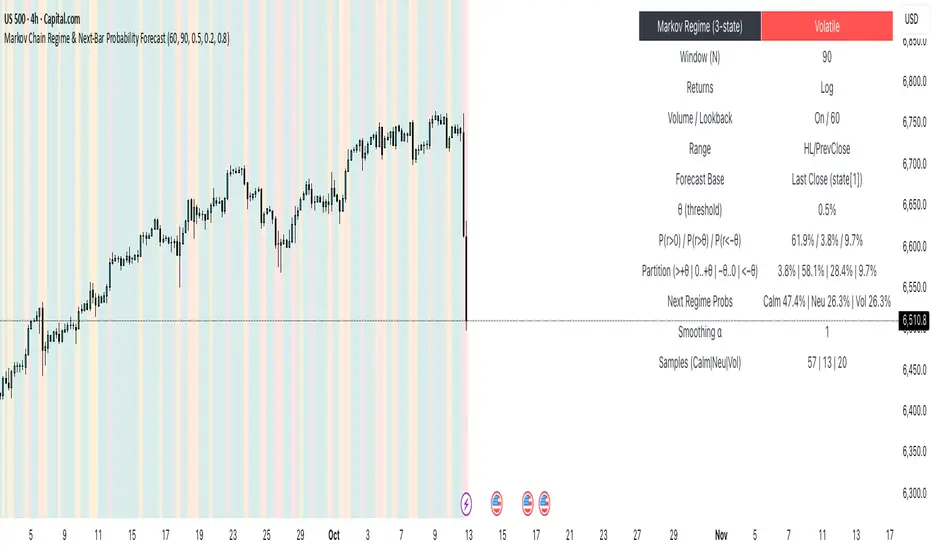
• P(next r < −θ)
• A 4-bucket split of next-bar outcomes (>+θ | 0..+θ | −θ..0 | <−θ)
• Next-regime probabilities: Calm | Neutral | Volatile
🧠 Why the math is strong
• Markov regimes: Markets cluster in volatility “moods.” We learn a 3-state regime S∈{Calm, Neutral, Volatile} with a transition matrix A, where A = P(Sₜ₊₁=j | Sₜ=i).
• Condition on the future state: We estimate event odds given the next regime j—
q_pos(j)=P(rₜ₊₁>0 | Sₜ₊₁=j), q_gt(j)=P(rₜ₊₁>+θ | Sₜ₊₁=j), q_lt(j)=P(rₜ₊₁<−θ | Sₜ₊₁=j)—
and mix them with transitions from the current (or frozen) state sNow:
P(event) = Σⱼ A · q(event | j).
This mixture-of-regimes view (HMM-style one-step prediction) ties next-bar outcomes to where volatility is likely headed.
• Statistical hygiene: Laplace/Beta smoothing, minimum-sample gating, and unconditional fallbacks keep estimates stable. Heavy computations run on confirmed bars; “Freeze at close” avoids intrabar flicker.
📊 What each value means
• Regime label & background: 🟩 Calm, 🟧 Neutral, 🟥 Volatile — quick read of market context.
• P(next r > 0): Directional tilt for the very next bar.
• P(next r > +θ): Odds of an outsized positive move beyond θ.
• P(next r < −θ): Odds of an outsized negative move beyond −θ.
• Partition row: Distributes next-bar probability across four intuitive buckets; they ≈ sum to 100%.
• Next Regime Probs: Likelihood of switching to Calm/Neutral/Volatile on the next bar (row of A for the current/frozen state).
• Samples row: How many next-bar samples support each next-state estimate (a confidence cue).
• Smoothing α: The Laplace prior used to stabilize binary event rates.
⚙️ Inputs you control
• Returns: Log (default) or %
• Include Volume (z-score) + lookback
• Include Range (HL/PrevClose)
• Rolling window N (transitions & estimates)
• θ as percent (e.g., 0.5%)
• Freeze forecast at last close (recommended)
• Display toggles (plots, partition, samples)
🎯 How to use it
• Volatility awareness & sizing: Rising P(next regime = Volatile) → consider smaller size, wider stops, or skipping marginal entries.
• Breakout preparation: Elevated P(next r > +θ) highlights environments where range expansion is more likely; pair with your setup/trigger.
• Defense for mean-reversion: If P(next r < −θ) lifts while you’re late long (or P(next r > +θ) lifts while late short), tighten risk or wait for better context.
• Calibration tip: Start θ near your market’s typical bar size; adjust until “>+θ” flags truly meaningful moves for your timeframe.
📝 Method notes & limits
Activity features (|r|, volume z, range) are standardized; only positive z’s feed the composite activity score. Estimates adapt to instrument/timeframe; rare regimes or small windows increase variance (hence smoothing, sample gating, fallbacks). This is a context/forecast tool, not a standalone signal—combine with your entry/exit rules and risk management.
🧩 Strategies too
We also develop full strategy versions that use these probabilities for entries, filters, and position sizing. Like this publication if you’d like us to release the strategy edition next.
⚠️ Disclaimer
Educational use only. Not financial advice. Markets involve risk. Past performance does not guarantee future results.
Cyclic Reversal Engine [AlgoPoint]Overview
Most indicators focus on price and momentum, but they often ignore a critical third dimension: time. Markets move in rhythmic cycles of expansion and contraction, but these cycles are not fixed; they speed up in trending markets and slow down in choppy conditions.
The Cyclic Reversal Engine is an advanced analytical tool designed to decode this rhythm. Instead of relying on static, lagging formulas, this indicator learns from past market behavior to anticipate when the current trend is statistically likely to reach its exhaustion point, providing high-probability reversal signals.
It achieves this by combining a sophisticated time analysis with a robust price-action confirmation.
How It Works: The Core Logic
The indicator operates on a multi-stage process to identify potential turning points in the market.
1. Market Regime Analysis (The Brain): Before analyzing any cycles, the indicator first diagnoses the current "personality" of the market. Using a combination of the ADX, Choppiness Index, and RSI, it classifies the market into one of three primary regimes:
- Trending: Strong, directional movement.
- Ranging: Sideways, non-directional chop.
- Reversal: An over-extended state (overbought/oversold) where a turn is imminent.
2. Adaptive Cycle Learning (The "Machine Learning" Aspect): This is the indicator's smartest feature. It constantly analyzes past cycles by measuring the bar-count between significant swing highs and swing lows. Crucially, it learns the average cycle duration for each specific market regime. For example, it learns that "in a strong trending market, a new swing low tends to occur every 35 bars," while "in a ranging market, this extends to 60 bars."
3. The Countdown & Timing Signal: The indicator identifies the last major swing high or low and starts a bar-by-bar countdown. Based on the current market regime, it selects the appropriate learned cycle length from its memory. When the bar count approaches this adaptive target, the indicator determines that a reversal is "due" from a timing perspective.
4. Price Confirmation (The Trigger): A signal is never generated based on timing alone. Once the timing condition is met (the cycle is "due"), the indicator waits for a final price-action confirmation. The default confirmation is the RSI entering an extreme overbought or oversold zone, signaling momentum exhaustion. The signal is only triggered when Time + Price Confirmation align.
How to Use This Indicator
- The Dashboard: The panel in the bottom-right corner is your command center.
- Market Regime: Shows the current market personality analyzed by the engine.
- Adaptive Cycle / Bar Count: This is the core of the indicator. It shows the target cycle length for the current regime (e.g., 50) and the current bar count since the last swing point (e.g., 45). The background turns orange when the bar count enters the "due zone," indicating that you should be on high alert for a reversal.
- BUY/SELL Signals: A label appears on the chart only when the two primary conditions are met:
The timing is right (Bar Count has reached the Adaptive Cycle target).
The price confirms exhaustion (RSI is in an extreme zone).
A BUY signal suggests a downtrend cycle is likely complete, and a SELL signal suggests an uptrend cycle is likely complete.
Key Settings
- Pivot Lookback: Controls the sensitivity of the swing point detection. Higher values will identify more significant, longer-term cycles.
- Market Regime Engine: The ADX, Choppiness, and RSI settings can be fine-tuned to adjust how the indicator classifies the market's personality.
- Require Price Confirmation: You can toggle the RSI confirmation on or off. It is highly recommended to keep it enabled for higher-quality signals.

Markov 3D Trend AnalyzerMarkov 3D Trend Analyzer
🔹 What Is a Markov State?
A Markov chain models systems as states with probabilities of transitioning from one state to another. The key property is memorylessness: the next state depends only on the current state, not the full past history. In financial markets, this allows us to study how conditions tend to persist or flip — for example, whether a green candle is more likely to be followed by another green or by a red.
🔹 How This Indicator Uses It
The Markov 3D Trend Analyzer tracks three independent Markov chains:
Direction Chain (short-term): Probability that a green/red candle continues or reverses.
Volatility Chain (mid-term): Probability of volatility staying Low/Medium/High or transitioning between them.
Momentum Chain (structural): Probability of momentum (Bullish, Neutral, Bearish) persisting or flipping.
Each chain is updated dynamically using exponentially weighted probabilities (EMA), which balance the law of large numbers (stability) with adaptivity to new market conditions.
The indicator then classifies each chain’s dominant state and combines them into an actionable summary at the bottom of the table (e.g. “📈 Bullish breakout,” “⚠️ Choppy bearish fakeouts,” “⏳ Trend squeeze / possible reversal”).
🔹 Settings
Direction Lookback / Volatility Lookback / Momentum Lookback
Control the rolling window length (sample size) for each chain. Larger = smoother but slower to adapt.
EMA Weight
Adjusts how much weight is given to recent transitions vs. older history. Lower values adapt faster, higher values stabilize.
Table Position
Choose where the table is displayed on your chart.
Table Size
Adjust the font size for readability.
🔹 How To Consider Using
Contextual tool: Use the summary row to understand the current market condition (trending, mean-reverting, expanding, compressing, continuation, fakeout risk).
Complementary filter: Combine with your existing strategies to confirm or filter signals. For example:
📈 If your breakout strategy fires and the summary says Bullish breakout, that’s confirmation.
⚠️ If it says Choppy fakeouts, be cautious of traps.
Visualization aid: The table lets you see how probabilities shift across direction, volatility, and momentum simultaneously.
⚠️ This indicator is not a signal generator. It is designed to help interpret market states probabilistically. Always use in conjunction with broader analysis and risk management.
🔹 Disclaimer
This script is for educational and informational purposes only. It does not constitute financial advice or a recommendation to buy or sell any security, cryptocurrency, or instrument. Trading involves risk, and past probabilities or behaviors do not guarantee future outcomes. Always conduct your own research and use proper risk management.

ATAI Triangles — Volume-Based & Price Pattern Analysis (v1.01)ATAI Triangles — Volume-Based & Price Pattern Analysis (v1.01)
Overview
ATAI Triangles identifies two synchronized triangle structures — Hi-Lo-Hi (HLH) and Lo-Hi-Lo (LHL) — and analyzes them both geometrically and volumetrically. For each triangle, volume is split between its two legs (segments), providing interpretable insights into buyer vs seller activity along each path.
The idea is that certain geometric shapes, when paired with volume distribution on each leg, can reveal patterns worth exploring. Users are encouraged to share their observations and interpretations in the TradingView comments section so that more aspects of these triangle combinations can be discovered collectively.
Extra (for fun)
For a bit of entertainment, we’ve included a symbolic “hexagram” glyph that appears when both triangle types align in a particular way — it’s just a visual nod to geometry and has no predictive or trading value.
Interface & data clarity
- Inputs and parameters are organized by function (pattern geometry, volume analysis, visuals, HUD, labels).
- Each input includes tooltips explaining its purpose, units, and possible effects on calculations.
- All on-chart objects (polylines, labels, connectors) are named and colored to reflect their role, with volume values formatted in engineering notation (K, M, B).
- HUD columns and label texts use concise terms and consistent units, so that every displayed value is directly traceable to a calculation in the code.
- Daily and lower-timeframe volume series are clearly separated, with update logic documented to indicate intrabar provisional values vs finalized bar-close values.
Usage notes
Designed to be used alongside other indicators and chart tools for context; it is not a standalone signal generator.
All Buy/Sell volumes are absolute (non-negative); Δ = Buy − Sell.
Intrabar values update live and finalize at bar close (no repaint after close).
Disclaimer
For research, discussion, and educational purposes only. This is not financial advice and does not guarantee any outcome. Trade at your own risk.

Gann Ultimate Time-Price Squares Method V 1.0This Script is an outcome of my Passion towards Gann Theory and his Methodology towards Trading.
The Script is still Evolving.So wait for more updates....
# Complete Trading Guide: Gann Time-Price Squares Indicator
## 🎯 Core Trading Philosophy
**Gann's Key Principle**: "When time and price come together, a change in trend occurs."
Your indicator identifies these critical moments where **Time = Price**, creating high-probability trading opportunities.
---
## 📊 Setup & Configuration
### Recommended Settings by Timeframe
| Timeframe | Pivot Lookback | Min Price Move | Tolerance | Use Case |
|-----------|---------------|----------------|-----------|----------|
| **1-5 min** | 5-8 bars | 0.5-1.0 | 1.0-2.0 | Scalping |
| **15-30 min** | 8-12 bars | 1.0-3.0 | 1.5-2.5 | Day Trading |
| **1-4 hour** | 10-15 bars | 2.0-5.0 | 2.0-3.0 | Swing Trading |
| **Daily** | 15-25 bars | 5.0-20.0 | 3.0-5.0 | Position Trading |
### Initial Setup Steps
1. **Add indicator** to your chart
2. **Set lookback period** based on your timeframe
3. **Adjust tolerance** - start with 2.0 and fine-tune
4. **Enable all visualizations** initially
5. **Position info table** where it doesn't block price action
---
## 🚀 Trading Strategies
### Strategy 1: Square Completion Reversal Trading
#### **Long Entry Setup**
```
CONDITIONS:
✅ Bullish square completes (green box appears)
✅ Info table shows "✅ COMPLETED" status
✅ Price bounces off square's bottom edge
✅ Volume increases on bounce
✅ RSI < 30 (oversold confirmation)
ENTRY: Market buy when price breaks above square's top edge
STOP: Below square's bottom edge (-2 ATR)
TARGET: Next resistance level or 1:2 Risk/Reward
```
#### **Short Entry Setup**
```
CONDITIONS:
✅ Bearish square completes (red box appears)
✅ Info table shows "✅ COMPLETED" status
✅ Price rejects square's top edge
✅ Volume increases on rejection
✅ RSI > 70 (overbought confirmation)
ENTRY: Market sell when price breaks below square's bottom edge
STOP: Above square's top edge (+2 ATR)
TARGET: Next support level or 1:2 Risk/Reward
```
### Strategy 2: Gann Angle Trend Following
#### **1x1 Angle (45°) - The Master Angle**
- **Most Important**: This is Gann's primary trend line
- **Bullish**: Price above 1x1 = uptrend intact
- **Bearish**: Price below 1x1 = downtrend intact
- **Break**: 1x1 angle break = major trend change
#### **Multi-Angle Confluence Trading**
```
STRONG BULLISH SIGNAL:
✅ Price above 1x1 angle (45°)
✅ Bouncing off 2x1 angle (support)
✅ Volume increasing
✅ Multiple angles pointing up
ENTRY: Buy on 2x1 angle bounce
STOP: Below 1x2 angle
TARGET: Next angle resistance
```
### Strategy 3: Projection Trading (Forming Squares)
#### **Anticipation Strategy**
```
SETUP IDENTIFICATION:
👀 Info table shows "⚡ FORMING" status
👀 Progress bar > 70%
👀 P/T Ratio approaching 1.00
👀 Price approaching projected completion zone
ENTRY PREPARATION:
- Set alerts for projected completion levels
- Prepare for reversal at projection zone
- Watch for volume confirmation
- Monitor momentum indicators
```
## 📈 Step-by-Step Trading Process
### Phase 1: Market Analysis (Before Trading)
1. **Check Market Trend**: Look at info table trend indicator
2. **Identify Active Pivots**: Note last significant high/low
3. **Assess Volatility**: High volatility = larger stops needed
4. **Review Completed Squares**: These become support/resistance zones
### Phase 2: Trade Setup Identification
1. **Monitor Forming Squares**: Watch progress bars in info table
2. **Check Gann Angles**: Are they supporting or opposing your bias?
3. **Confirm with Volume**: Look for volume spikes at key levels
4. **Set Alerts**: Use TradingView alerts for completion zones
### Phase 3: Trade Execution
1. **Wait for Confirmation**: Don't trade on projections alone
2. **Enter on Breakout**: Price breaking square boundaries
3. **Set Stops Immediately**: Use square edges as stop levels
4. **Scale Out**: Take partial profits at angle intersections
### Phase 4: Trade Management
1. **Trail Stops**: Use Gann angles as trailing stop levels
2. **Monitor Progress**: Watch for new square formations
3. **Exit Signals**: New squares in opposite direction
4. **Review Performance**: Analyze win/loss against square accuracy
---
## 🎯 High-Probability Setups
### Setup A: Double Confirmation
```
BULLISH EXAMPLE:
1. Bullish square completes at major support
2. Price bounces off 1x1 Gann angle
3. Volume surge confirms reversal
4. RSI divergence present
PROBABILITY: 75-80%
RISK/REWARD: 1:3 typical
```
### Setup B: Angle Breakout
```
BEARISH EXAMPLE:
1. Price breaks below 1x1 angle
2. Bearish square forming below break
3. Multiple angles now resistance
4. Volume confirms breakdown
PROBABILITY: 70-75%
RISK/REWARD: 1:2.5 typical
```
### Setup C: Time Cycle Convergence
```
REVERSAL EXAMPLE:
1. Square completion at time cycle high/low
2. Multiple Gann angles converging
3. Momentum divergence
4. Volume climax
PROBABILITY: 80-85%
RISK/REWARD: 1:4 possible
```
---
## ⚠️ Risk Management Rules
### Position Sizing
- **Conservative**: 1-2% risk per trade
- **Aggressive**: 2-3% risk per trade
- **Never exceed**: 5% total portfolio risk
### Stop Loss Guidelines
- **Completed Squares**: Opposite edge + 1 ATR
- **Gann Angles**: Below/above angle + 0.5 ATR
- **Projections**: 50% of square height
### Take Profit Targets
- **Target 1**: Next Gann angle (1:1 R/R)
- **Target 2**: Next completed square (1:2 R/R)
- **Target 3**: Major S/R level (1:3 R/R)
---
## 📊 Reading the Info Table for Trading
### Market Trend Section
```
📈 BULLISH → Look for long setups
📉 BEARISH → Look for short setups
➡️ NEUTRAL → Wait for direction
```
### Volatility Status
```
🔥 HIGH → Larger stops needed
⚡ ELEVATED → Normal stops
😴 LOW → Tighter stops possible
📊 NORMAL → Standard approach
```
### Square Progress Monitoring
```
✅ COMPLETED → Ready to trade
⚡ FORMING → Prepare for setup
🔥 ACTIVE → Monitor closely
⏳ WAITING → No immediate action
```
### P/T Ratio Interpretation
```
🎯 Perfect (0.8-1.2) → High probability setup
⚡ Good (0.6-1.4) → Moderate probability
⚠️ Watch (outside range) → Lower probability
```
---
## 🔄 Common Trading Scenarios
### Scenario 1: Trend Continuation
**Setup**: Price pulls back to completed square in uptrend
**Action**: Buy at square support with 1x1 angle confirmation
**Management**: Trail stop below each new square formation
### Scenario 2: Reversal Trading
**Setup**: Multiple squares complete at major S/R
**Action**: Fade the move when price rejects square edges
**Management**: Quick profits, tight stops
### Scenario 3: Breakout Trading
**Setup**: Price consolidates in square, then breaks out
**Action**: Trade breakout direction with volume confirmation
**Management**: Use opposite square edge as stop
---
## 📱 Alert Setup Recommendations
### Critical Alerts
1. **Square Completion**: "Gann Square Completed - Check for reversal"
2. **1x1 Angle Break**: "Master angle broken - Trend change possible"
3. **Projection Reached**: "Forming square at 90% - Prepare for reversal"
4. **Multi-Angle Touch**: "Price at angle confluence - High probability setup"
---
Remember: **Gann analysis is both art and science**. The indicator provides the mathematical framework, but successful trading requires patience, discipline, and continuous learning. Start with small positions while you master the methodology!

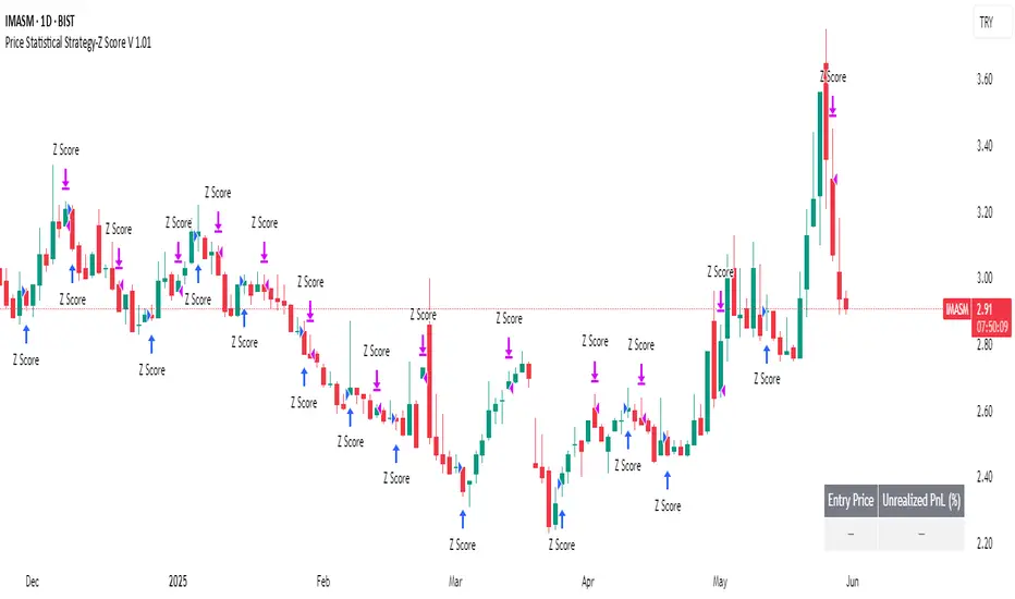
Price Statistical Strategy-Z Score V 1.01
Price Statistical Strategy – Z Score V 1.01
Overview
A technical breakdown of the logic and components of the “Price Statistical Strategy – Z Score V 1.01”.
This script implements a smoothed Z-Score crossover mechanism applied to the closing price to detect potential statistical deviations from local price mean. The strategy operates solely on price data (close) and includes signal spacing control and momentum-based candle filters. No volume-based or trend-detection components are included.
Core Methodology
The strategy is built on the statistical concept of Z-Score, which quantifies how far a value (closing price) is from its recent average, normalized by standard deviation. Two moving averages of the raw Z-Score are calculated: a short-term and a long-term smoothed version. The crossover between them generates long entries and exits.
Signal Conditions
Entry Condition:
A long position is opened when the short-term smoothed Z-Score crosses above the long-term smoothed Z-Score, and additional entry conditions are met.
Exit Condition:
The position is closed when the short-term Z-Score crosses below the long-term Z-Score, provided the exit conditions allow.
Signal Gapping:
A minimum number of bars (Bars gap between identical signals) must pass between repeated entry or exit signals to reduce noise.
Momentum Filter:
Entries are prevented during sequences of three or more consecutively bullish candles, and exits are prevented during three or more consecutively bearish candles.
Z-Score Function
The Z-Score is calculated as:
Z = (Close - SMA(Close, N)) / STDEV(Close, N)
Where N is the base period selected by the user.
Input Parameters
Enable Smoothed Z-Score Strategy
Enables or disables the Z-Score strategy logic. When disabled, no trades are executed.
Z-Score Base Period
Defines the number of bars used to calculate the simple moving average and standard deviation for the Z-Score. This value affects how responsive the raw Z-Score is to price changes.
Short-Term Smoothing
Sets the smoothing window for the short-term Z-Score. Higher values produce smoother short-term signals, reducing sensitivity to short-term volatility.
Long-Term Smoothing
Sets the smoothing window for the long-term Z-Score, which acts as the reference line in the crossover logic.
Bars gap between identical signals
Minimum number of bars that must pass before another signal of the same type (entry or exit) is allowed. This helps reduce redundant or overly frequent signals.
Trade Visualization Table
A table positioned at the bottom-right displays live PnL for open trades:
Entry Price
Unrealized PnL %
Text colors adapt based on whether unrealized profit is positive, negative, or neutral.
Technical Notes
This strategy uses only close prices — no trend indicators or volume components are applied.
All calculations are based on simple moving averages and standard deviation over user-defined windows.
Designed as a minimal, isolated Z-Score engine without confirmation filters or multi-factor triggers.
Market Timing(Mastersinnifty)Overview
Market Timing (Mastersinnifty) is a proprietary visualization tool designed to help traders study historical market behavior through structural pattern similarity.
The script analyzes the most recent session’s price action and identifies the closest-matching historical sequence among thousands of past patterns. Once a match is found, the script projects the subsequent historical price path onto the current chart for easy visual reference.
Unlike traditional indicators, Market Timing (Mastersinnifty) does not generate trade signals. Instead, it offers a unique historical scenario analysis based on quantified structural similarity.
---
How It Works
- The script captures the last 20 closing prices and compares them to historical price sequences from the past 8000 bars.
- Similarity is computed using the Euclidean distance formula (sum of squared differences) between the current pattern and historical candidates.
- Upon finding the most similar past pattern, the subsequent historical movement is normalized relative to session opening and plotted onto the current chart using projection lines.
- The projection automatically adapts to intraday, daily, weekly, or monthly timeframes, with the option for manual or automatic projection length settings.
- Session start detection is handled automatically based on volume thresholds and price-time analysis to adjust for market openings across different instruments.
---
Key Features
- Historical Pattern Matching: Quantitative matching of the most similar past price structure.
- Dynamic Projections: Visualizes likely historical scenarios based on past market behavior.
- Auto/Manual Projection Length: Flexible control over the number of projected bars.
- Multi-Timeframe Support: Works seamlessly across intraday, daily, weekly, and monthly charts.
- Purely Visual Context: Designed to support human decision-making without replacing it with automatic trade signals.
---
Who Can Benefit
- Traders studying market structure repetition and price symmetry.
- Visual thinkers who prefer scenario-based planning over fixed indicator systems.
- Intraday, swing, and position traders looking for historical context to complement price action, volume, and momentum studies.
---
How to Use
- Apply the script to any asset — including indices, stocks, commodities, forex, or crypto.
- Select your preferred timeframe.
- Choose "Auto" or "Custom" for the projection length.
- Observe the projected lines:
- Upward slope = Historical bullish continuation.
- Downward slope = Historical bearish continuation.
- Flat movement = Historical sideways movement.
- Combine insights with volume, support/resistance, and price action for better decision-making.
---
Important Notes
- This script does not predict the future. It offers a visual reference based on historical similarity.
- Always validate projected scenarios with live market conditions.
- Market structure evolves; past behavior may not repeat under new market dynamics.
- Use this tool for educational and research purposes only.
---
Disclaimer
This is not financial advice. The Market Timing (Mastersinnifty) tool is intended for research and educational purposes only. Trading involves risk, and past performance does not guarantee future results. Always apply sound risk management practices.

Future Candle Reversal Projection (Mastersinnifty)Overview
This tool identifies potential future market reversal zones by dynamically projecting pivot-based swing patterns forward in time. Unlike traditional ZigZag indicators that only reflect past movements, this indicator anticipates probable future turning points based on historical swing periodicity.
---
Key Features
- Forward Projections: Calculates and projects future swing zones based on detected pivot distances.
- Customizable Detection: Adjust the ZigZag depth for different trading styles (scalping, swing, position).
- Dynamic Updates: Real-time recalibration as new pivots form.
- Clean Visual Markers: Projects reversal estimates as intuitive labels and dotted lines.
---
How it Works
The indicator identifies significant swing highs and lows using a user-defined ZigZag depth setting. It measures the time (bars) and price characteristics of the latest swing movement. Using this pattern, it projects forward estimated reversal points at consistent intervals. Midpoint price levels between the last high and low are used for each future projection.
---
Who Can Benefit
- Intraday and swing traders seeking advanced planning zones.
- Technical analysts relying on pattern periodicity.
- Traders who wish to combine projected reversal markers with their own risk management strategies.
---
Disclaimer
This tool is an analytical and educational utility. It does not predict markets with certainty. Always combine it with your own analysis and risk management. Past behavior does not guarantee future results.

Autocorrelation Price Forecasting [The Quant Science]Discover how to predict future price movements using autocorrelation and linear regression models to identify potential trading opportunities.
An advanced model to predict future price movements using autocorrelation and linear regression. This script helps identify recurring market cycles and calculates potential gains, with clear visual signals for quick and informed decisions.
Main function
This script leverages an autocorrelation model to estimate the future price of an asset based on historical price relationships. It also integrates linear regression on percentage returns to provide more accurate predictions of price movements.
Insights types
1) Red label on a green candle: Bearish forecast and swing trading opportunity.
2) Red label on a red candle: Bearish forecast and trend-following opportunity.
3) Green label on a red candle: Bullish forecast and swing trading opportunity.
4) Green label on a green candle: Bullish forecast and trend-following opportunity.
IMPORTANT!
The indicator displays a future price forecast. When negative, it estimates a future price drop.
When positive, it estimates a future price increase.
Key Features
Customizable inputs
Analysis Length: number of historical bars used for autocorrelation calculation. Adjustable between 1 and 200.
Forecast Colors: customize colors for bullish and bearish signals.
Visual insights
Labels: hypothetical gains or losses are displayed as labels above or below the bars.
Dynamic coloring: bullish (green) and bearish (red) signals are highlighted directly on the chart.
Forecast line: A continuous line is plotted to represent the estimated future price values.
Practical applications
Short-term Trading: identify repetitive market cycles to anticipate future movements.
Visual Decision-making: colored signals and labels make it easier to visualize potential profit or loss for each trade.
Advanced Customization: adjust the data length and colors to tailor the indicator to your strategies.
Limitations
Prediction price models have some limitations. Trading decisions should be made with caution, considering additional market factors and risk management strategies.

Doubled Numbered Square of Nine Progression | RegressionThe Doubled Number Square of Nine Progression | Regression Indicator enables forecasting of support and resistance levels using the SQ9 progression or regression from a user-selected pivot price. The indicator also plots adjustable pivots on both the chart and the Square of Nine.
How to use to forecast support and resistance levels:
1. Select a Pivot Point: Choose a top or bottom pivot to use as the starting point. Select High or Low in the indicator to set the correct price to the pivot.
2. Set Price Increment or Decrement: Select a price increment to advance the starting price on the Square of Nine (for example 1 or -0.01).
3. Rotate to add or decrease the number of rungs on the Square on Nine: Rotate the Square of Nine and adjust the dimensions. The horizontal levels correlate to the rotation of the Square of Nine.
4. Plot Levels: Select a Square of Nine angle to plot the support and resistance levels based on the selected increments. These levels auto expand and decrease depending on the number of rotations in step 3. The price values from each of the selected diagonal or cardinal cross are applied to the chart with labels on both left and right. Left labels represent the cell the time variable and the right label is price.
5. Review Levels: Conduct a simple review of the plotted support and resistance levels in relation to recent market pivots.
6. Identify Correlations: Identify the Square of Nine cardinal cross or diagonal cross angle that correlates with the most market pivots.
7. The indicator plots user-adjustable pivots on both candles/bars and displays their placement on the Square of Nine in both Progression and Regression. The close price is plotted on the Square of Nine in real-time with a white background. This helps users identify which angles the highs and lows favor from the selected pivot. The pivot levels' colors can be adjusted.
Each market has its tendencies, favoring specific angles from the cardinal or diagonal cross. The basic idea is to choose between the diagonal cross and cardinal cross angles to forecast support and resistance levels.
Settings:
Overview:
Example on Forecasting Support and resistance level using this indicator:
In the image above, I'm progressing from the significant low at a rate of $200 per cell. Based on the plotted pivots, I've selected the 315-degree angle on the diagonal cross as it aligns with a few recent pivots. Now, I've drawn a vertical line to show that as we add rungs to the Square of Nine, we introduce support and resistance levels based on the identified angle that aligns with these early pivots from the low.
In the image below, I've moved forward in time to show how the initial angle selected based on the early pivot forecasted support and resistance levels around the high in BTC. Do not expect the price to turn sharply at the levels the indicator generates, but use it to help identify SQ9 levels that may form market turns. As P. Mikula mentions in his work, "The Square of Nine successfully defines market price swings but it does not make the market form pivots."
This indicator includes enhancements made to the Gann Square of Nine indicator originally created by @ThiagoSchmitz.
This indicator is inspired by the methodologies detailed by Patrick Mikula in his book " The Definitive Guide to Forecasting using W.D Gann's Square of Nine ." I recommend checking it out. He also mentions another use case as a Price and Time chart in his " Gann Scientific Method Unveiled, Volume 2 ." FYI, I am not affiliated with Patrick Mikula in any way.
Known Issues:
Close price plotted on the Square of Nine in Regression "from a high pivot" takes a current candle to close in order to be plotted. Progression works as expected.

AiTrend Pattern Matrix for kNN Forecasting (AiBitcoinTrend)The AiTrend Pattern Matrix for kNN Forecasting (AiBitcoinTrend) is a cutting-edge indicator that combines advanced mathematical modeling, AI-driven analytics, and segment-based pattern recognition to forecast price movements with precision. This tool is designed to provide traders with deep insights into market dynamics by leveraging multivariate pattern detection and sophisticated predictive algorithms.
👽 Core Features
Segment-Based Pattern Recognition
At its heart, the indicator divides price data into discrete segments, capturing key elements like candle bodies, high-low ranges, and wicks. These segments are normalized using ATR-based volatility adjustments to ensure robustness across varying market conditions.
AI-Powered k-Nearest Neighbors (kNN) Prediction
The predictive engine uses the kNN algorithm to identify the closest historical patterns in a multivariate dictionary. By calculating the distance between current and historical segments, the algorithm determines the most likely outcomes, weighting predictions based on either proximity (distance) or averages.
Dynamic Dictionary of Historical Patterns
The indicator maintains a rolling dictionary of historical patterns, storing multivariate data for:
Candle body ranges, High-low ranges, Wick highs and lows.
This dynamic approach ensures the model adapts continuously to evolving market conditions.
Volatility-Normalized Forecasting
Using ATR bands, the indicator normalizes patterns, reducing noise and enhancing the reliability of predictions in high-volatility environments.
AI-Driven Trend Detection
The indicator not only predicts price levels but also identifies market regimes by comparing current conditions to historically significant highs, lows, and midpoints. This allows for clear visualizations of trend shifts and momentum changes.
👽 Deep Dive into the Core Mathematics
👾 Segment-Based Multivariate Pattern Analysis
The indicator analyzes price data by dividing each bar into distinct segments, isolating key components such as:
Body Ranges: Differences between the open and close prices.
High-Low Ranges: Capturing the full volatility of a bar.
Wick Extremes: Quantifying deviations beyond the body, both above and below.
Each segment contributes uniquely to the predictive model, ensuring a rich, multidimensional understanding of price action. These segments are stored in a rolling dictionary of patterns, enabling the indicator to reference historical behavior dynamically.
👾 Volatility Normalization Using ATR
To ensure robustness across varying market conditions, the indicator normalizes patterns using Average True Range (ATR). This process scales each component to account for the prevailing market volatility, allowing the algorithm to compare patterns on a level playing field regardless of differing price scales or fluctuations.
👾 k-Nearest Neighbors (kNN) Algorithm
The AI core employs the kNN algorithm, a machine-learning technique that evaluates the similarity between the current pattern and a library of historical patterns.
Euclidean Distance Calculation:
The indicator computes the multivariate distance across four distinct dimensions: body range, high-low range, wick low, and wick high. This ensures a comprehensive and precise comparison between patterns.
Weighting Schemes: The contribution of each pattern to the forecast is either weighted by its proximity (distance) or averaged, based on user settings.
👾 Prediction Horizon and Refinement
The indicator forecasts future price movements (Y_hat) by predicting logarithmic changes in the price and projecting them forward using exponential scaling. This forecast is smoothed using a user-defined EMA filter to reduce noise and enhance actionable clarity.
👽 AI-Driven Pattern Recognition
Dynamic Dictionary of Patterns: The indicator maintains a rolling dictionary of N multivariate patterns, continuously updated to reflect the latest market data. This ensures it adapts seamlessly to changing market conditions.
Nearest Neighbor Matching: At each bar, the algorithm identifies the most similar historical pattern. The prediction is based on the aggregated outcomes of the closest neighbors, providing confidence levels and directional bias.
Multivariate Synthesis: By combining multiple dimensions of price action into a unified prediction, the indicator achieves a level of depth and accuracy unattainable by single-variable models.
Visual Outputs
Forecast Line (Y_hat_line):
A smoothed projection of the expected price trend, based on the weighted contribution of similar historical patterns.
Trend Regime Bands:
Dynamic high, low, and midlines highlight the current market regime, providing actionable insights into momentum and range.
Historical Pattern Matching:
The nearest historical pattern is displayed, allowing traders to visualize similarities
👽 Applications
Trend Identification:
Detect and follow emerging trends early using dynamic trend regime analysis.
Reversal Signals:
Anticipate market reversals with high-confidence predictions based on historically similar scenarios.
Range and Momentum Trading:
Leverage multivariate analysis to understand price ranges and momentum, making it suitable for both breakout and mean-reversion strategies.
Disclaimer: This information is for entertainment purposes only and does not constitute financial advice. Please consult with a qualified financial advisor before making any investment decisions.

Kalman PredictorThe **Kalman Predictor** indicator is a powerful tool designed for traders looking to enhance their market analysis by smoothing price data and projecting future price movements. This script implements a Kalman filter, a statistical method for noise reduction, to dynamically estimate price trends and velocity. Combined with ATR-based confidence bands, it provides actionable insights into potential price movement, while offering clear trend and momentum visualization.
---
#### **Key Features**:
1. **Kalman Filter Smoothing**:
- Dynamically estimates the current price state and velocity to filter out market noise.
- Projects three future price levels (`Next Bar`, `Next +2`, `Next +3`) based on velocity.
2. **Dynamic Confidence Bands**:
- Confidence bands are calculated using ATR (Average True Range) to reflect market volatility.
- Visualizes potential price deviation from projected levels.
3. **Trend Visualization**:
- Color-coded prediction dots:
- **Green**: Indicates an upward trend (positive velocity).
- **Red**: Indicates a downward trend (negative velocity).
- Dynamically updated label displaying the current trend and velocity value.
4. **User Customization**:
- Inputs to adjust the process and measurement noise for the Kalman filter (`q` and `r`).
- Configurable ATR multiplier for confidence bands.
- Toggleable trend label with adjustable positioning.
---
#### **How It Works**:
1. **Kalman Filter Core**:
- The Kalman filter continuously updates the estimated price state and velocity based on real-time price changes.
- Projections are based on the current price trend (velocity) and extend into the future (Next Bar, +2, +3).
2. **Confidence Bands**:
- Calculated using ATR to provide a dynamic range around the projected future prices.
- Indicates potential volatility and helps traders assess risk-reward scenarios.
3. **Trend Label**:
- Updates dynamically on the last bar to show:
- Current trend direction (Up/Down).
- Velocity value, providing insight into the expected magnitude of the price movement.
---
#### **How to Use**:
- **Trend Analysis**:
- Observe the direction and spacing of the prediction dots relative to current candles.
- Larger spacing indicates a potential strong move, while clustering suggests consolidation.
- **Risk Management**:
- Use the confidence bands to gauge potential price volatility and set stop-loss or take-profit levels accordingly.
- **Pullback Detection**:
- Look for flattening or clustering of dots during trends as a signal of potential pullbacks or reversals.
---
#### **Customizable Inputs**:
- **Kalman Filter Parameters**:
- `lookback`: Adjusts the smoothing window.
- `q`: Process noise (higher values make the filter more reactive to changes).
- `r`: Measurement noise (controls sensitivity to price deviations).
- **Confidence Bands**:
- `band_multiplier`: Multiplies ATR to define the range of confidence bands.
- **Visualization**:
- `show_label`: Option to toggle the trend label.
- `label_offset`: Adjusts the label’s distance from the price for better visibility.
---
#### **Examples of Use**:
- **Scalping**: Use on lower timeframes (e.g., 1-minute, 5-minute) to detect short-term price trends and reversals.
- **Swing Trading**: Identify pullbacks or continuations on higher timeframes (e.g., 4-hour, daily) by observing the prediction dots and confidence bands.
- **Risk Assessment**: Confidence bands help visualize potential price volatility, aiding in the placement of stops and targets.
---
#### **Notes for Traders**:
- The **Kalman Predictor** does not predict the future with certainty but provides a statistically informed estimate of price movement.
- Confidence bands are based on historical volatility and should be used as guidelines, not guarantees.
- Always combine this tool with other analysis techniques for optimal results.
---
This script is open-source, and the Kalman filter logic has been implemented uniquely to integrate noise reduction with dynamic confidence band visualization. If you find this indicator useful, feel free to share your feedback and experiences!
---
#### **Credits**:
This script was developed leveraging the statistical principles of Kalman filtering and is entirely original. It incorporates ATR for dynamic confidence band calculations to enhance trader usability and market adaptability.

Holt-Winters Forecast BandsDescription:
The Holt-Winters Adaptive Bands indicator combines seasonal trend forecasting with adaptive volatility bands. It uses the Holt-Winters triple exponential smoothing model to project future price trends, while Nadaraya-Watson smoothed bands highlight dynamic support and resistance zones.
This indicator is ideal for traders seeking to predict future price movements and visualize potential market turning points. By focusing on broader seasonal and trend data, it provides insight into both short- and long-term market directions. It’s particularly effective for swing trading and medium-to-long-term trend analysis on timeframes like daily and 4-hour charts, although it can be adjusted for other timeframes.
Key Features:
Holt-Winters Forecast Line: The core of this indicator is the Holt-Winters model, which uses three components — level, trend, and seasonality — to project future prices. This model is widely used for time-series forecasting, and in this script, it provides a dynamic forecast line that predicts where price might move based on historical patterns.
Adaptive Volatility Bands: The shaded areas around the forecast line are based on Nadaraya-Watson smoothing of historical price data. These bands provide a visual representation of potential support and resistance levels, adapting to recent volatility in the market. The bands' fill colors (red for upper and green for lower) allow traders to identify potential reversal zones without cluttering the chart.
Dynamic Confidence Levels: The indicator adapts its forecast based on market volatility, using inputs such as average true range (ATR) and price deviations. This means that in high-volatility conditions, the bands may widen to account for increased price movements, helping traders gauge the current market environment.
How to Use:
Forecasting: Use the forecast line to gain insight into potential future price direction. This line provides a directional bias, helping traders anticipate whether the price may continue along a trend or reverse.
Support and Resistance Zones: The shaded bands act as dynamic support and resistance zones. When price enters the upper (red) band, it may be in an overbought area, while the lower (green) band may indicate oversold conditions. These bands adjust with volatility, so they reflect the current market conditions rather than fixed levels.
Timeframe Recommendations:
This indicator performs best on daily and 4-hour charts due to its reliance on trend and seasonality. It can be used on lower timeframes, but accuracy may vary due to increased price noise.
For traders looking to capture swing trades, the daily and 4-hour timeframes provide a balance of trend stability and signal reliability.
Adjustable Settings:
Alpha, Beta, and Gamma: These settings control the level, trend, and seasonality components of the forecast. Alpha is generally the most sensitive setting for adjusting responsiveness to recent price movements, while Beta and Gamma help fine-tune the trend and seasonal adjustments.
Band Smoothing and Deviation: These settings control the lookback period and width of the volatility bands, allowing users to customize how closely the bands follow price action.
Parameters:
Prediction Length: Sets the length of the forecast, determining how far into the future the prediction line extends.
Season Length: Defines the seasonality cycle. A setting of 14 is typical for bi-weekly cycles, but this can be adjusted based on observed market cycles.
Alpha, Beta, Gamma: These parameters adjust the Holt-Winters model's sensitivity to recent prices, trends, and seasonal patterns.
Band Smoothing: Determines the smoothing applied to the bands, making them either more reactive or smoother.
Ideal Use Cases:
Swing Trading and Trend Following: The Holt-Winters model is particularly suited for capturing larger market trends. Use the forecast line to determine trend direction and the bands to gauge support/resistance levels for potential entries or exits.
Identifying Reversal Zones: The adaptive bands act as dynamic overbought and oversold zones, giving traders potential reversal areas when price reaches these levels.
Important Notes:
No Buy/Sell Signals: This indicator does not produce direct buy or sell signals. It’s intended for visual trend analysis and support/resistance identification, leaving trade decisions to the user.
Not for High-Frequency Trading: Due to the nature of the Holt-Winters model, this indicator is optimized for higher timeframes like the daily and 4-hour charts. It may not be suitable for high-frequency or scalping strategies on very short timeframes.
Adjust for Volatility: If using the indicator on lower timeframes or more volatile assets, consider adjusting the band smoothing and prediction length settings for better responsiveness.
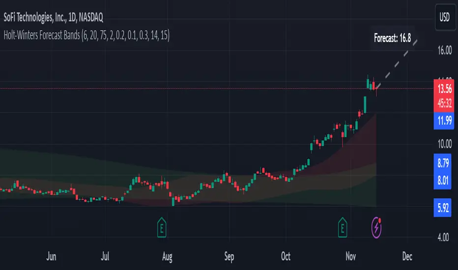
Trend Forecasting - The Quant Science🌏 Trend Forecasting | ENG 🌏
This plug-in acts as a statistical filter, adding new information to your chart that will allow you to quickly verify the direction of a trend and the probability with which the price will be above or below the average in the future, helping you to uncover probable market inefficiencies.
🧠 Model calculation
The model calculates the arithmetic mean in relation to positive and negative events within the available sample for the selected time series. Where a positive event is defined as a closing price greater than the average, and a negative event as a closing price less than the average. Once all events have been calculated, the probabilities are extrapolated by relating each event.
Example
Positive event A: 70
Negative event B: 30
Total events: 100
Probabilities A: (100 / 70) x 100 = 70%
Probabilities B: (100 / 30) x 100 = 30%
Event A has a 70% probability of occurring compared to Event B which has a 30% probability.
🔍 Information Filter
The data on the graph show the future probabilities of prices being above average (default in green) and the probabilities of prices being below average (default in red).
The information that can be quickly retrieved from this indicator is:
1. Trend: Above-average prices together with a constant of data in green greater than 50% + 1 indicate that the observed historical series shows a bullish trend. The probability is correlated proportionally to the value of the data; the higher and increasing the expected value, the greater the observed bullish trend. On the other hand, a below-average price together with a red-coloured data constant show quantitative data regarding the presence of a bearish trend.
2. Future Probability: By analysing the data, it is possible to find the probability with which the price will be above or below the average in the future. In green are classified the probabilities that the price will be higher than the average, in red are classified the probabilities that the price will be lower than the average.
🔫 Operational Filter .
The indicator can be used operationally in the search for investment or trading opportunities given its ability to identify an inefficiency within the observed data sample.
⬆ Bullish forecast
For bullish trades, the inefficiency will appear as a historical series with a bullish trend, with high probability of a bullish trend in the future that is currently below the average.
⬇ Bearish forecast
For short trades, the inefficiency will appear as a historical series with a bearish trend, with a high probability of a bearish trend in the future that is currently above the average.
📚 Settings
Input: via the Input user interface, it is possible to adjust the periods (1 to 500) with which the average is to be calculated. By default the periods are set to 200, which means that the average is calculated by taking the last 200 periods.
Style: via the Style user interface it is possible to adjust the colour and switch a specific output on or off.
🇮🇹Previsione Della Tendenza Futura | ITA 🇮🇹
Questo plug-in funge da filtro statistico, aggiungendo nuove informazioni al tuo grafico che ti permetteranno di verificare rapidamente tendenza di un trend, probabilità con la quale il prezzo si troverà sopra o sotto la media in futuro aiutandoti a scovare probabili inefficienze di mercato.
🧠 Calcolo del modello
Il modello calcola la media aritmetica in relazione con gli eventi positivi e negativi all'intero del campione disponibile per la serie storica selezionata. Dove per evento positivo si intende un prezzo alla chiusura maggiore della media, mentre per evento negativo si intende un prezzo alla chiusura minore della media. Calcolata la totalità degli eventi le probabilità vengono estrapolate rapportando ciascun evento.
Esempio
Evento positivo A: 70
Evento negativo B: 30
Totale eventi : 100
Formula A: (100 / 70) x 100 = 70%
Formula B: (100 / 30) x 100 = 30%
Evento A ha una probabilità del 70% di realizzarsi rispetto all' Evento B che ha una probabilità pari al 30%.
🔍 Filtro informativo
I dati sul grafico mostrano le probabilità future che i prezzi siano sopra la media (di default in verde) e le probabilità che i prezzi siano sotto la media (di default in rosso).
Le informazioni che si possono rapidamente reperire da questo indicatore sono:
1. Trend: I prezzi sopra la media insieme ad una costante di dati in verde maggiori al 50% + 1 indicano che la serie storica osservata presenta un trend rialzista. La probabilità è correlata proporzionalmente al valore del dato; tanto più sarà alto e crescente il valore atteso e maggiore sarà la tendenza rialzista osservata. Viceversa, un prezzo sotto la media insieme ad una costante di dati classificati in colore rosso mostrano dati quantitativi riguardo la presenza di una tendenza ribassista.
2. Probabilità future: analizzando i dati è possibile reperire la probabilità con cui il prezzo si troverà sopra o sotto la media in futuro. In verde vengono classificate le probabilità che il prezzo sarà maggiore alla media, in rosso vengono classificate le probabilità che il prezzo sarà minore della media.
🔫 Filtro operativo
L' indicatore può essere utilizzato a livello operativo nella ricerca di opportunità di investimento o di trading vista la capacità di identificare un inefficienza all'interno del campione di dati osservato.
⬆ Previsione rialzista
Per operatività di tipo rialzista l'inefficienza apparirà come una serie storica a tendenza rialzista, con alte probabilità di tendenza rialzista in futuro che attualmente si trova al di sotto della media.
⬇ Previsione ribassista
Per operatività di tipo short l'inefficienza apparirà come una serie storica a tendenza ribassista, con alte probabilità di tendenza ribassista in futuro che si trova attualmente sopra la media.
📚 Impostazioni
Input: tramite l'interfaccia utente Input è possibile regolare i periodi (da 1 a 500) con cui calcolare la media. Di default i periodi sono impostati sul valore di 200, questo significa che la media viene calcolata prendendo gli ultimi 200 periodi.
Style: tramite l'interfaccia utente Style è possibile regolare il colore e attivare o disattivare un specifico output.
Nasan Moving Average with ForecastThe "Nasan Moving Average with Forecast" indicator is a technical analysis forecasting tool that combines the principles of historical data analysis and random walk theory. It calculates a customized moving average (Nasan Moving Average) by integrating price data and statistical measures and projects future price points by generating forecast values within calculated volatility bounds, creating a dynamic and insightful visualization of potential market movements. This indicator to blend past market behavior with probabilistic future trends to enhance forecasting.
Input Parameters:
len: Differencing length (default 21, Use a minimum of 5 and for lower time frames less than 15 min use values between 300 -3000)
len1: Correction Factor Length 1 (default 21, this determines the length of the MA you want , eg. 10 MA, 50 MA, 100 MA, )
len2: Correction Factor Length 2 (default 9, this works best if it is ~ </=1/2 of len1 )
len3: Smoothing Length (default 5, I would not change this and only use if I want to introduce lag where you want to use it for cross over strategies).
forecast_points: Number of points to forecast (default 30).
m: Multiplier for standard deviation (default 2.5).
bl: Block length for calculating max/min values (default 100).
use_calculated_max_min: Boolean to decide whether to use calculated max/min values.
Nasan Moving Average Calculation:
Calculates the simple moving average (mean) and standard deviation (sd) of the typical price (hlc3).
Computes intermediate variables (a, b, c, etc.) based on log transformation and cumulative sum.
Applies weighted moving averages (wma) to these intermediate variables to smooth them and derive the final value c6.
Plots c6 as the Nasan Moving Average if the bar is confirmed. To learn more see Nasan Moving Average.
Forecast Points Calculation:
Calculates maximum (max_val) and minimum (min_val) values for the forecast, either using a fixed value or based on standard deviation and a multiplier.
Initializes an array to store forecast values and creates polyline objects for plotting.
If the current bar is one of the last three bars and confirmed:
Clears and reinitializes the polyline.
Initializes the first forecast value from the cumulative sum c.
Generates subsequent forecast values using a random value within the range .
Updates the forecast array and plots the forecast points as an orange curved polyline.
Plotting Max/Min Values:
Plots max_val and min_val as green and red lines, respectively, to indicate the bounds of the forecast range.
Components of the Forecasting Model
Historical Dependence:
Nasan Moving Average Calculation: The script calculates a custom moving average (c6) that incorporates historical price data (hlc3), standard deviations (sd), and weighted moving averages (wma). This part of the code processes historical data to create a smoothed representation of the price trend.
Max/Min Value Calculation: The maximum (max_val) and minimum (min_val) values for the forecast can be calculated based on the historical standard deviation of a transformed variable b over a block length (bl). This introduces historical volatility into the bounds for the forecast.
Random Walk Model:
Random Value Generation: Within the forecast points calculation, a random value (random_val) is generated for each forecast point within the range . This random value introduces stochasticity into the model, characteristic of a random walk process.
Cumulative Sum for Forecasting: The script uses a cumulative sum (prev_f + random_val) to generate the next forecast point (next_f). This is a typical approach in random walk models where each new point is based on the previous point plus some random noise.
Explanation of the Forecast Model
Random Walk Characteristics: Each new forecast point is generated by adding a random value to the previous point, making the model a random walk with drift, where the drift is influenced by historical correction factors (c1, c4).
Historical and Statistical Dependence: The bounds of the random values and the initial conditions are derived from historical data, ensuring that the forecast respects historical volatility and trends.
The forecasting model in the script is a hybrid approach: It uses a random walk to generate future points, characterized by adding random values to the previous forecasted value.
The historical and statistical dependence is incorporated through initial conditions, scaling factors, and bounds derived from historical price data and its statistical properties.
This combination ensures that the forecasts are not purely stochastic but are grounded in historical price behavior, making the model more robust and potentially more accurate in reflecting market conditions.
Liquidity Dependent Price Stability AlgorithmThe Liquidity Dependent Price Stability (LDPS) indicator is designed to measure liquidity levels on an equity and, from those measurements, provide Bullish or Bearish outlooks for future price action. These outlooks are given via reporting the equity's Liquidity Condition and Liquidity Flow.
Interpretation
Liquidity Condition (LC) and Liquidity Flow (LF) measurements are displayed with color-specific chart colors and/or with text output.
LC can be reported as "Weak Bullish", "Bullish", or "Strong Bullish" for Bullish outlooks and "Weak Bearish", "Bearish" or "Strong Bearish" for Bearish outlooks. LC can also just be reported as "Bullish" or "Bearish".
Bullish LCs have a statistical correlation with future price appreciation, and Bearish LCs have a statistical correlation with price depreciation. When LC is “Bullish”, the price is likely to go up, and if LC is “Bearish”, the price is likely to go down.
Liquidity Flow (LF) is a measure of how LC is changing. When LC is becoming more bullish, LF is reported as “Improving”. When LC is becoming more bearish, LF is reported as “Worsening”. LF is only displayed via text output.
Settings and Configurations
LDPS Sensitivity and Reactivity: Determines if you want LDPS to be more sensitive to changing conditions or less sensitive. This choice affects how certain LDPS is when forming its future outlooks. LDPS achieves this increase in sensitivity and reactivity by lowering the bar for what LDPS considers a significant change.
Aggressive : LDPS will optimize reporting early changes in LC and LF at the expensive of accuracy. Aggressive is good for low-risk trading styles that prefer to exit a position early rather than deal with increased risk of oppositional movement.
Balanced : LDPS will try to balance reporting changes in LC and LF with maintaining accuracy. Balanced style is a good setting to start out with and is applicable across the widest range of equity’s and timeframes.
Conservative : LDPS will optimize accuracy over being sensitive to changes in LC or LF. Conservative is a good choice for lower timeframes and traders who only want to change or exit positions with the greatest confidence.
LDPS Reporting Style: Determines how you want LC to be reported.
Simplified : LDPS will only report LC as “Bullish” or “Bearish”.
Full : LDPS will increase its reporting details and include the “Strong” and “Weak” pre-fixes, when appropriate.
LDPS Candle Coloring: There are three different ways that LC can be reported on the chart via coloring.
LDPS Candle Replacement: This will replace the chart’s default candles with those created by LDPS. Note: In order to see LDPS’ candles and not the chart’s, you have to disable to chart’s candles. This can be done in Settings -> Symbol and unchecking “Body”, “Borders” and “Wick” boxes.
LDPS Candle Coloring: This will just color the bodies of the chart’s default candles. Note: This setting should not have the chart’s candle’s disabled.
LDPS Background Coloring: This will color the chart’s background rather than any candles.
LDPS Text Output: LC and LF are reported via a text box that can be moved several places on the chart, or the text box can be removed.
LDPS Measurements – Display: When selected, LC and LF will be reported via the text box.
LDPS Measurement – Text Location: Determines where the text box with LC and LF are located.
LDPS Measurement – Text Size: Determines the size of LC and LF within the text box.
LDPS Measurement – Background Color: Determines the background color of the text box with LC and LF.
LDPS Condition Color Selection – Bullish / Bearish: Color selection for each type of LC. Note: If the Simplified reporting style is selected, the “Full Bullish” and “Full Bearish” are the bullish and bearish color choices, respectively.
Frequently Asked Questions:
Where can I get additional Information?
Please check the “Author’s Instructions” section below.
Where can I find the results of the LDPS research?
Please check the “Author’s Instructions” section below.
Help! Something’s not working!
Apologies. Please see the email listed in “Author’s Instructions” below and let’s get started on solving the issue.
Which Sensitivity setting should I use?
The author’s preference is Conservative in most cases, but the answer for you depends on your preferred style.
An analogy might help: the aggressive setting will ensure LDPS is early to the party – every party. Of the parties that really kick off, you can be certain LDPS is there, but they had to visit a several of parties before finding the right one.
The Conservative setting won’t bring LDPS to every party – it will gladly stay at the one it’s at but when it detects the next real big hit, LDPS will move to that party instead. It won’t be the first one there, but it is definitely earlier than most.
Should I use the Full or Simplified reporting style?
Depending on how engaged you are with the particular equity or position, either choice can be beneficial. The Full reporting style will let you detect changes in LC before they might show with the Simplified reporting style. Some enjoy the additional data, some (like the Author) enjoy keeping things simple.
I can see LDPS’ colors in the chart’s candlesticks when the settings are open, but not when the settings are closed. How come?
If you are using the “LDPS Candle Replacement” setting, be sure to turn off the Chart’s default candles by right-clicking on the chart, going to Settings, then Symbol and then un-checking “Body”, “Border” and “Wick”. This should fix the issue.
I think there’s a bug – where do I report it?
Thank you for reaching out about a potential bug or issue! Please see the email below in “Author’s Instructions” to report the issue.