"机械革命无界15+时不时闪屏"に関するスクリプトを検索
(JS) Ultimate RSISo my goal here was to combine all of my RSI ideas into a single indicator in order to make kind of a "Swiss Army Knife" version of the Relative Strength Index ...
------------------------------------------------------------------------------------------------------------------------------------------------------------------------------------------------------------------------------------------------------------------
So, let's begin with the first RSI indicator I made, which is the RSIDVW (Divergence/Volume Weighted);
To rephrase my original post, the "divergence/volume weighted" portion is meant to expand upon the current RSI format by adding more variables into the equation.
The standard RSI is based off one value that you select (open, close, OHLC4, HLC3, etc.) while this version takes three variables into account.
The default setting is to have RSI normal without anything added to it (Divergence Weight = 0)
1st - it takes the standard variable that RSI normally uses.
2nd - it factors RSI divergence by taking the RSI change % and price change % to form a ratio. Using this ratio, I duplicated the RSI formula and created a divergence RS to be factored in with the standard price RS .
3rd - it takes Relative Volume and amplifies/weakens the move based upon volume confirmation. (So if Relative Volume for a price bar is 1.0, the RSI plot would be the same as it normally would)
So to explain the parameters
- Relative Volume Length: This uses the RV length you specify to determine spikes in volume (or lack of volume ), which then is added into the formula to influence the strength of the RSI move
- RV x Divergence: This is how I calculated the original formula, but you can leave this unchecked to turn Relative Volume off, or apply elsewhere.
- RV x RS: There's two sides, Divergence RS and Standard RS - these check marks allow you to select which part you prefer to be multiplied by Relative Volume .
Checking neither turns off Relative Volume , while checking both amplifies its effects by placing it on both sides of the equation.
-Divergence Weight: This controls how much the DVW portion of the formula influences the RSI plot. As I referred to earlier, default is 0 making RSI normal. The Scale is 0-2, so 1.0 would be the same as 50%.
When I do have DVW on, I generally set it to 0.5
-SMA Divergence: To smooth, or not to smooth, that is the question. UJsing an SMA here is much smoother in my opinon, but leaving it unchecked runs it through an RMA the same way standard RSI is calculated.
-Show Fractal Channel: This allows you to see the whole fractal channel around the RSI (This portion of the code, compliments of the original Ricardo Santos fractal script)
------------------------------------------------------------------------------------------------------------------------------------------------------------------------------------------------------------------------------------------------------------------
The next portion of the script is adding a "Slow RSI"...
This is rather simple really, it allows you to add a second RSI plot so that you can watch for crossovers between fast and slow lines.
-Slow RSI: This turns on the second RSI Plot.
-Slow RSI Length: This determines the length of the second RSI Plot.
------------------------------------------------------------------------------------------------------------------------------------------------------------------------------------------------------------------------------------------------------------------
Pivot Point RSI was something a friend of mine requested I make which turned out pretty cool, I thought... It is also available in this indicator.
-Pivot Points: Selecting this enables the rest of the pivot point related parts of the script
If Pivot Points isn't selected, none of the following things will work
-Plot Pivot: Plots the pivot point .
-Plot S1/R1: Plots S1/R1.
-Plot S2/R2: Plots S2/R2.
-Plot S3/R3: Plots S3/R3.
-Plot S4/R4: Plots S4/R4.
-Plot S5/R5: Plots S5/R5.
-Plot Halfway Points: Plots a line between each pivot .
-Show Pivot Labels: Shows the proper label for each pivot .
When using intraday charts, from a 15 minute interval or less the pivots are calculated based on a single days worth of price action, above that the distance expands.
Here are the current resolutions Pivot Points will work with:
Minutes - 1 , 2, 3, 5, 10, 13, 15, 20, 30, 39, 78, 130, 195
Hours - 1, 2, 3, 4, 5, 6
Daily
Weekly
Currently not available on seconds or monthly
------------------------------------------------------------------------------------------------------------------------------------------------------------------------------------------------------------------------------------------------------------------
Background Colors
Background Colors: I have six color schemes I created for this which can be toggled here (they can be edited).
Gray Background for Dark Mode: Having this on looks much better when using dark mode on your charts.
------------------------------------------------------------------------------------------------------------------------------------------------------------------------------------------------------------------------------------------------------------------
Now finally the last portion, Fibonacci Levels
-Fibonacci Levels: This is off, by default, which then uses the standard levels on RSI (30-50-70). When turned on, it removes these and marks fib levels from 0.146 through 0.886.
------------------------------------------------------------------------------------------------------------------------------------------------------------------------------------------------------------------------------------------------------------------
So the quick rundown:
Ultimate RSI contains "divergence/volume weighted" modifications, a slow RSI plot, pivot points , and Fibonacci levels all while auto-plotting divergence and having the trend illustrated in the background colors.
RSI has always been my "go to" indicator, so I hope you all enjoy this as much as I do!
15M 2PM-3PM High/LowThis script will draw horizontal lines based on the high and low values between 2PM and 3PM (inclusive 2PM & 3PM) on 15 minute time frame. This indicator can be used in 15 minute time frame to plot the high and low lines correctly. This indicator can be used for previous day 2PM-3PM range breakout or breakdown trades.

Donchian FibsSo this is donchian channel with its fibs level
the TF is set to 1440 min to show daily trend
the highs and lows of the channel is shown
so why this shit?
I like sometime to play on lower TF lets say 5 min chart or 15 min chart
So if I reduce the TF to 60 on 5 or 15 min chart I can get more realistic fib system then the regular that we normaly use
So you need to play with TF to get the best result for your chart :)

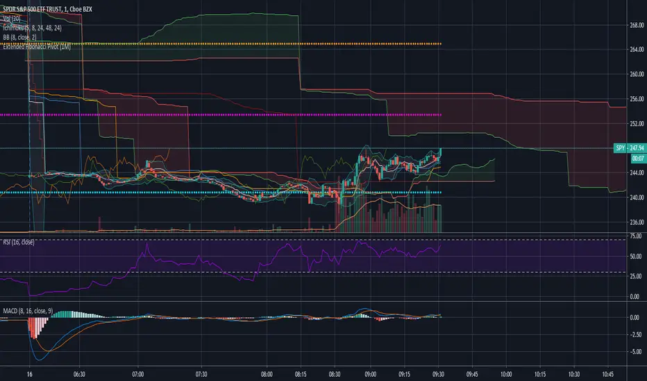
Extended Fibonacci PivotEditable Fibonacci Pivots. 0.236, 0.382, 0.618, 0.786, 1.000. Easy to extend further if needed. Can be used with intervals from 1 minute to 1 Day.
A Few Recommended timeframes:
1 minute chart - 15 Minute Pivot Timeframe
3 minute chart - 1 Hour Timeframe or Daily Timeframe
15 Minutes to < 60 Minutes - Daily Timeframe
1 Hour to 4 Hour - Weekly Timeframe
Daily - Monthly Timeframe
Dual Ichimoku CloudDual Ichimoku cloud
Now you don't need to switch between time frames to see cloud support/resistance!
Configure cloud as you wish then set ratio.
Example Rations
3 Minutes to 15 Minutes = 5
15 Minutes to 1 Hour = 4
1 Day to 1 Week = 5

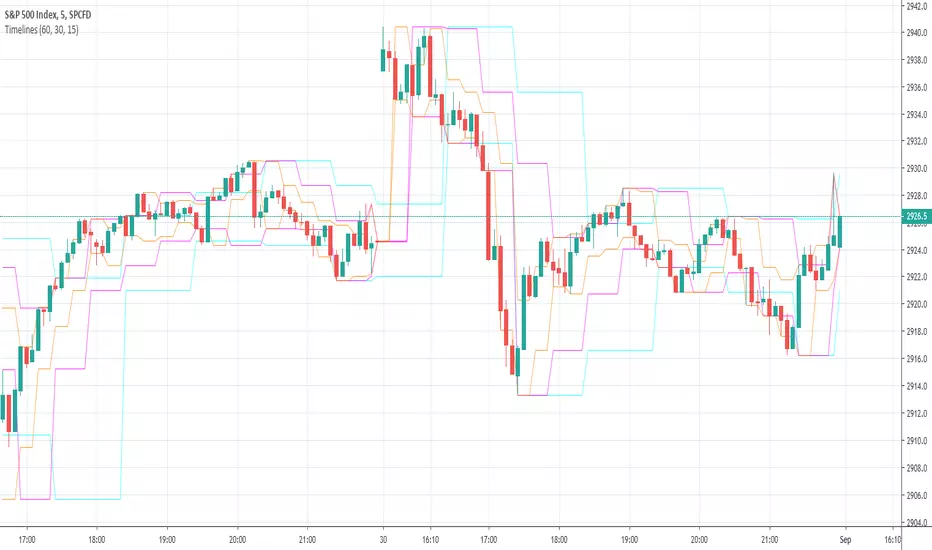
Timelines-Buschi
English:
This is a little, simple script I made upon request from a user.
It shows the highs ad lows of up to three custom timelines (e. g. 60 min, 30 min and 15 min) within a chart.
Deutsch:
Dies ist ein kleines, einfaches Skript, das ich auf Anfrage eines Nutzers erstellt habe.
Es zeigt die Hochs und Tiefs von bis zu drei individueller Zeitreihen (z. B. 60 min, 30 min und 15 min) innerhalb eines Charts.
Supertrend MTF LAG ISSUEThis script based on
we all use Super trend but it main issue is the lag as it buy too late or sell too late
using Deavaet study of Heat map MTF we can do a little trick
if you look on his study you can see that major signal for example will happen in the time frame before it happen at larger time frame
so in this example if signal at MTF 30 min and signal at MTF 60 min happen at the same time at 2 hours or 4 hours candles then this signal are more likely to be true then random signal at each time frame specific.
since we use shorter time frame on larger time frame we can remove the lag issue that make supertrend not so effective
In this example I set the signal to be MTF 30 +60 om 2 hour TF , can be good also for 4 hour candles..
So you get the signal to close inside the larger candle
now if you want to make on even shorter TF then change the code to 15 and 30 MTF on candles on 1 hour
or 1 and 5 min on 30 min or 15 min

RVOL - R4RocketRelative volume or RVOL for short is an indicator that is used to measure how 'In Play' the stock is. Simply put, it helps to quantify how interested everybody is in the given stock - higher the value, higher the interest and hence higher is the probability for movement in the stock.
I have tried to create RVOL (Relative Volume ) Indicator as per the description that I read on SMB Capital blog. The blog is a great resource.
...................................................................................................................................................................................
How to use the indicator - The indicator is meant for INTRADAY ONLY.
The indicator has following inputs -
1. RVOL Period - Value from 3 to 14 (Default Value = 4)
This is used to calculate the average volume over the given period of days. e.g. average volume for the last 5 days, last 3 days, last 10 days etc. NOTE - If you use higher RVOL Period on smaller timeframes, the code will give an error. So I recommend using 4 or lower for 5 min timeframe. (Nothing will work on 1 min chart and you can experiment for other timeframes.)
2. RVOL Sectional - True / False (Default Value = False)
If you check this box then you will be able to calculate the RVOL for a particular session (or between particular sessions) in that trading day.
What do I mean by session?
Well I have divided the trading day into 6 (almost) equally spaced sessions in time, i.e. 6 hours and 15 mins (for NSE - India) of trading day is divided into 1 hr - 1st session, 1 hr - 2nd session, 1 hr - 3rd session, 1 hr - 4th session, 1 hr - 5th session, 1 hr and 15 min - 6th session.
Before using 3rd and 4th inputs of indicator, RVOL Sectional box MUST BE CHECKED FIRST.
3. RVOL From Session - 1 to 6 (Default Value = 1)
4. RVOL To Session - 1 to 6 (Default Value = 2)
Now if you select 2 in "RVOL From Session" input and 3 in "RVOL To Session" input, the indicator will calculate RVOL for the 2nd and 3rd hour of the trading day. If you select 3 in both the inputs, then the indicator will give RVOL for the 3rd hour of the trading day.
5. RVOL Trigger - 0.2 to 10 (Default Value = 2)
Filter to find days having RVOL above that value. The indicator turns green (or colour of your choice) when RVOL is more than "RVOL Trigger".
...................................................................................................................................................................................
Hope this indicator will add some value in your trading endeavor.
“Only The Game, Can Teach You The Game” – Jesse Livermore
Yours sincerely,
R4Rocket
**If you have some awesome idea for improvement of the indicator - request you to update the code and share the same.

Sexy RSI for sexy tradersHello fellow sexy traders.
I was tired of constantly having to add my own horizontals/MAs to the default RSI so I decided to make this modification.
The default settings include channels from 40-80 (green horizontals) for a bullish range, and 20-60 (red horizontals) for the bearish range.
Also includes white line at 50 level, and blue horizontals at extremes (90 and 10).
If RSI stays in one of the red or green range that can signify the trend direction, as directed by Andrew Cardwell (inventor of the RSI).
If you wish for other levels to be included, just let me know! Comment on here or dm me on twitter @boss_charts and I can add the settings for you, so all you have to do is click a button and it will set it to your desired config. I want this to be a tool that is useful for heavy traders to save them time.
Additionally, in order to tell the level of the RSI and how overextended it might be, I added the setting for the RSI to change color depending on its level. Current settings are as follows:
Normal RSI (30-70) = PURPLE
Conventional Overbought/Oversold (30-20 + 70-80) = RED
1st extended (20-15 + 80-85) = PINK
2nd extended (15-10 + 85-90) = ORANGE
VERY EXTENDED (<10 + >90) = YELLOW
That way you can get an idea of how drastic a move is by the color alone. According to Dr. Cardwell, a drastic move to over/under extended can be a sign of strength.
Finally, there are the default MAs added that Mr. Cardwell defines as useful for defining the trend. These being the 9 MA and 45 EMA/WMA.
The strategy with these is to have the MAs on both price and RSI. If the 9MA is above the 45 MA on both price and RSI, then this is bullish and you can look for longs.
Conversely, if the 9 is below the 45 on both RSI and price that is bearish, and you can look for shorts.
I added the background color change for the points where the MAs cross each other, so you do not have to have the MAs fogging up your charts to know where they are relative to one another. This is similar to my MA cross indicator which contains the same functionality.
Never financial advice. Backtest it for yourself and find MA configurations that work for you.
Enjoy! Feel free to send feedback/requests whenever.

ADX +- DiThis Adx +-Di is just a complete version of what the ADX is supposed to signal.
So you have:
15 (contraction), 20 (threshold), 30 (expansion), 40 (resistance) levels.
Below 20 the price is not trending
Above 30 the price is trending
Below 15 price has been in contraction for too long
Between 20 and 30 price is in a "transition zone".
I finally added a "Resistance" level (40), which has to be adapted to best represent the historical levels where price usually encounters resistance, and where the price can be declared "overtrending", which means a return to lower levels is likely to happen.
I've chosen mild colors, and set the Adx Color to White, because I use black background, you can easily change that.
Enjoy
-Maurice

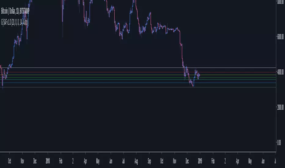
GoTiT|Simple Auto Fib v1.0Simple Auto Fib!
Notes:
1. Always set the trend manually! Don't rely on the auto trend detection.
2. The first parameter Length sets the number of candles back (left) to search for highs and lows from the current candle.
3. The High Offset parameter sets the number of candles back (left) to ignore/skip before searching for highs.
4. The Low Offset parameter sets the number of candles back (left) to ignore/skip before searching for lows.
5. The offset parameters change the behavior of the Length parameter.
Example 1:
Length = 100
High Offset = 0
Low Offset = 0
This is the default behavior, and the search for highs and lows occurs on the last 100 candles.
Example 2:
Length = 50
High Offset = 20 (Ignore the last 20 candles, and search for highs starting at candle 21 to 71 (or 50 candles back)
Low Offset = 15 (Ignore the last 15 candles, and search for lows starting at candle 16 to 66 (or 50 candles back)
In example 2, search starts on candle 21 for highs, and candle 16 for lows and extends 50 candles further back from there.
6. The Trend Detection parameter sets the number of candles back (left) to use in the trend calculations. Larger values give better "marco trend" detection. Smaller values give better "micro trend" detection. See note #1.
7. The white fib line is fib0. Assuming you correctly set the trend manually (or the trend is auto detected correctly), in a downtrend fib0 should be bellow the red fib line, and in an uptrend fib0 should be above the red fib line.
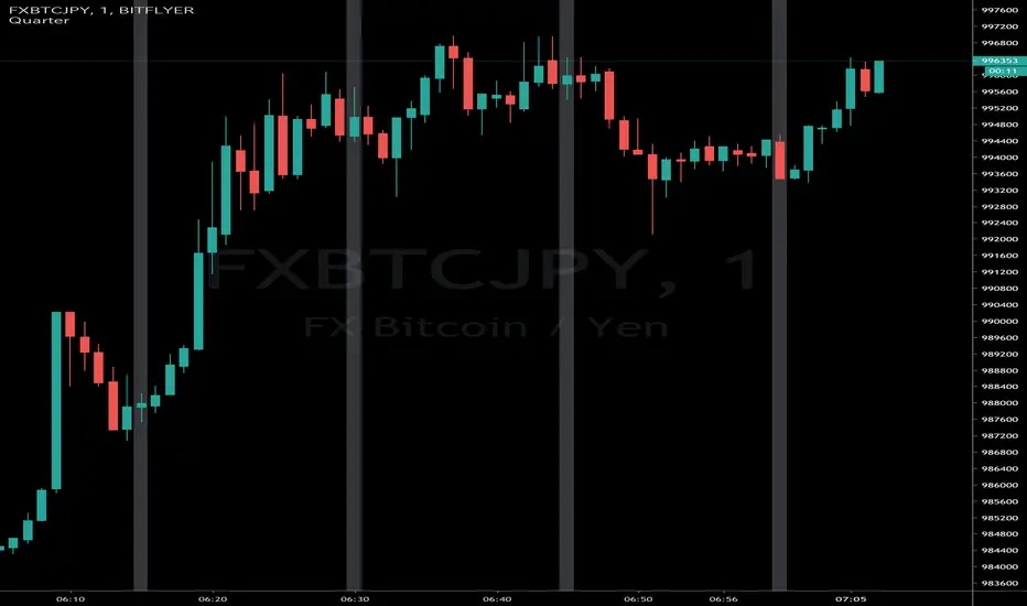
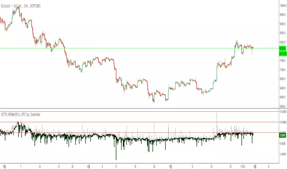
BITFLYER's SFD by CalendarHi guys, I am Calendar.
My first customized indicator is SFD difference in Bitflyer
Bitflyer exchange charges penalties to long postion if difference between FXBTC/JPY and BTC/JPY is more than 5, 10, 15, 20%
So, it is selling signal when the difference is higher than 5, 10, 15, 20%
Plz check “setting” -> “Scales” -> “Indicator Last Value”
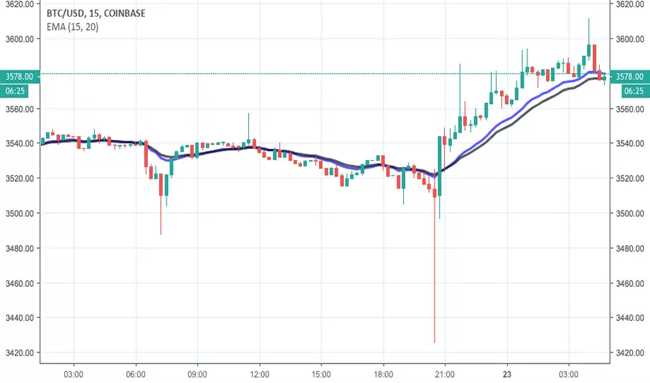
3 Linear Regression CurveFast 3LRC - 15/30/60 standard settings - 15/30 give a lot of noise, but give you a some time to prepare for the 60 to flip
Noro's OverCloud v1.2 MTFAdded big timeframe
MN = 1 month
W = 1 week
D = 1 day
240 = 4 hours
180 = 3 hours
120 = 2 hours
60 = 1 hours
30 = 30 min
15 = 15 min
etc...

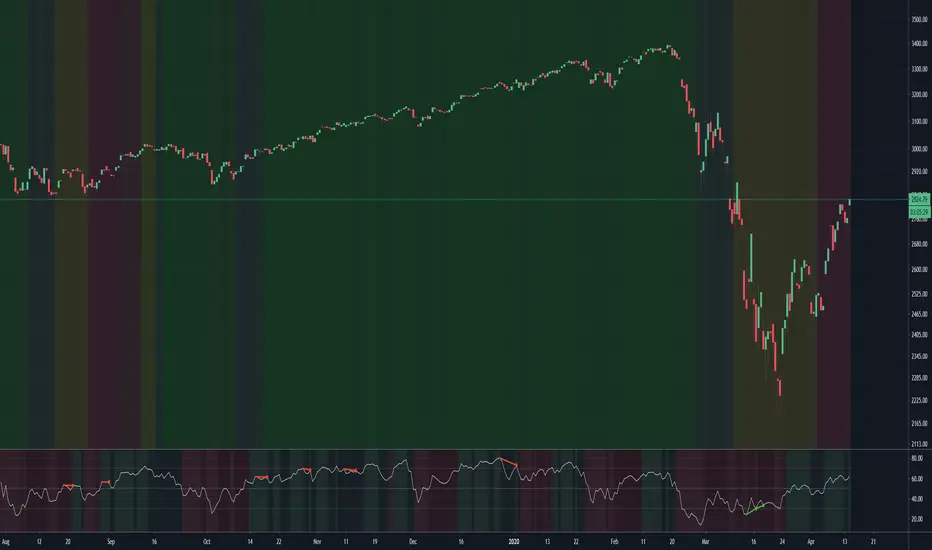
Fractal Resonance BarLazyBear's WaveTrend port has been praised for highlighting trend reversals with precision and punctuality (minimal lag). But strong "3rd Wave" trends can "embed" or saturate any oscillator flashing several premature crosses while stuck overbought/oversold. This happens when the trend stretches over a longer timescale than the oscillator's averaging window or filter time constant. Our solution: monitor many timescales. With Fractal Resonance Bar's rich color codings, strong wavefronts form across timescales and jump out like an approaching line of thunderclouds!
Fractal Resonance Bar color-codes the status of eight underlying stochastic oscillators, with each row averaging over twice the time of the row above.
Fractal Resonance Bar shifts its timescales along with your choice of main chart timescale:
1 minute chart: 1 minute through 128 minute (~2 hour) oscillators.
15 minute chart: 15 minute through 1920 minute (~32 hour) oscillators.
1 hour chart: 1 hour through 128 hour (~2 week) oscillators.
Daily chart: 1 day through 128 day (~4 month) oscillators.
The color map is configured as follows:
Hot Pink: Extreme Overbought (> 100%) rolled over to sell, but oscillators probably embedded with more upside (revert to Dark Green) possible after a pause.
Deep Red: Overbought (> 75%) crossover ripe for selling (validated when red spreads to timescales below).
Brown: Minor (< 75%) crossover sell from which could bounce back green or start a plunge toward gray/black.
Gray/Black: Mature (< -75%) sells turning full black in a plunge before the dawn.
Lime Green: Extreme Oversold (< -100%) and bouncing, though may yet bottom even lower.
Green: Oversold (< -75%) crossover ripe for buy. Green spreading to all timescales below will validate bottom is in.
Dark Green/Teal: Mature buy in overbought (> 75%) range, waiting for sell crossover to Hot Pink for a pause or correction.
White Stripes are Impulsive Trend Warning
Fractal Resonance Bar warns of oscillator embedding by showing white stripes when it detects strong, early surges in the timescale rows below.The white stripes usually accompany Hot Pink warning it's too early to go short, or Lime Green warning it's too early to go long.
Heeding these warnings will probably miss the exact top or bottom, but you're less likely to get overrun in a momentum move.
Usually the market gives us a second opportunity to short very close to the top or buy very close to the bottom after the warning white stripes have subsided.
NOTE: Recently rolled over Futures contracts may not have enough history for all oscillator calculations, in which case no bar colors will appear.
Tweakable Attributes
The default Channel Length, Stochastic Ratio Length and Lag Length work reasonably well on all timescales in our experience. Minor tweaks don't hurt but this may just overfit to a particular chart history.
We don't recommend changing the 75% Overbought and 100% Extreme Overbought default levels as these are ideal numbers relative to the underlying oscillator statistic calculations. But these settings can shift the color transition levels.
Embedded attribute controls the sensitivity/conservativeness of the white strip embedding detectors. Closer to 75 increases the warning sensitivity while closer to 100 decreases the aggressiveness of blocking white stripes.
Embed Separation also affects the white stripe sensitivity.
Row width increases each row's thickness to fill the available screen height you've afforded the bar.

Trend and Entry CCI ST15This is a T3 CCI with a fast and slow line as well as extreme lines, a -15,15 filter to make zero line rejections and crosses more mechanical and help weed out whipsaw. I will probably update description in the future and get into more detail about how the indicator is used but for now if you want more info look up woodie CCI patterns :) Good Luck!!
extended session - Regular Opening-Range- JayyOpening Range and some other scripts updated to plot correctly (see comments below.) There are three variations of the fibonacci expansion beyond the opening range and retracements within the opening range of the US Market session - I have not put in the script for the other markets yet.
The three scripts have different uses and strengths:
The extended session script (with the script here below) will plot the opening range whether you are using the extended session or the regular session. (that is to say whether "ext" in the lower right hand corner is highlighted or not.). While in the extended session the opening range has some plotting issues with periods like 13 minutes or any period that is not divisible into 330 mins with a round number outcome (eg 330/60 =5.5. Therefore an hour long opening range has problems in the extended session.
The pre session script is only for the premarket. You can select any opening range period you like. I have set the opening range to be the full premarket session. If you select a different session you will have to unselect "pre open to 9:30 EST for Opening Range?" in the format section. The script defaults to 15 minutes in the "period Of Pre Opening Range?". To go back to the 4 am to 9:30 pre opening range select "pre open to 9:30 EST for Opening Range?" there is no automatic 330 minute selection.
The past days offset script only works in 5 min or 15 minute period. It will show the opening range from up to 20 days past over the current days price action. Use this for the regular session only. 0 shows the current day's opening range. Use the positive integers for number of days back ie 1, 2, 3 etc not -1, -2, -3 etc. The script is preprogrammed to use the current day (0).
Scripts updated to plot correctly: One thing they all have in common is a way of they deal with a somewhat random problem that shifts the plots 4 hours in one direction or the other ie the plot started at 9:30 EST or 1:30PM EST. This issue started to occur approximately June 22, 2015 and impacts any script that tried to use "session" times to manage a plot in my scripts. The issue now seems to have been resolved during this past week.
Just in case the problem reoccurs I have added a "Switch session plot?" to each script. If the plot looks funny check or uncheck the "Switch session plot?" and see the difference. Of course if a new issue crops up it will likely require a different fix.
I have updated all of the scripts shown on this chart. If you are using a script of mine that suffers from the compiler issue then you will find an update on this chart. You can get any and all of the scripts by clicking on the small sideways wishbone on the left middle of the chart. You will see a dialogue box. Then click "make it mine". This will import all of the scripts to your computer and you can play around with them all to decide what you want and what you don't want. This is the easiest way to get all of the scripts in one fell swoop. It is also the easiest way for me to make all of the scripts available. I do not have all of the plots visible since it is too messy and one of the scripts (pre OR) is only for the regular session. To view the scripts click on the blue eye to the right of the script title to show it on this script. If you can only use the regular session. The scripts will all (with the exception of the pre OR) work fine.
If for any reason this script seems flakey refresh the page r try a slightly different period. I have noticed that sometimes randomly the script loves to return to the 5 min OR. This is a very new issue transient issue. As always if you see an issue please let me know.
Cheers Jayy
BB 100 with Barcolors6/19/15 I added confirmation highlight bars to the code. In other words, if a candle bounced off the lower Bollinger band, it needed one more close above the previous candle to confirm a higher probability that a change in investor sentiment has reversed. Same is true for upper Bollinger band bounces. I also added confirmation highlight bars to the 100 sma (the basis). The idea is that lower and upper bands are potential points of support and resistance. The same is true of the basis if a trend is to continue. 6/28/15 I added a plotshape to identify closes above/below TLine. One thing this system points out is it operates best in a trend reversal. Consolidations will whipsaw the indicator too much. I have found that when this happens, if using daily candles, switch to hourly, 30 min, etc., to catch a better signal. Nothing moves in a straight line. As with any indicator, it is a tool to be used in conjunction with the art AND science of trading. As always, try the indicator for a time so that you are comfortable enough to use real money. This is designed to be used with "BB 25 with Barcolors".

BB 25 with Barcolors6/19/15 I added confirmation highlight bars to the code. In other words, if a candle bounced off the lower Bollinger band, it needed one more close above the previous candle to confirm a higher probability that a change in investor sentiment has reversed. Same is true for upper Bollinger band bounces. I also added confirmation highlight bars to the 100 sma (the basis). The idea is that lower and upper bands are potential points of support and resistance. The same is true of the basis if a trend is to continue. 6/28/15 I added a plotshape to identify closes above/below TLine. One thing this system points out is it operates best in a trend reversal. Consolidations will whipsaw the indicator too much. I have found that when this happens, if using daily candles, switch to hourly, 30 min, etc., to catch a better signal. Nothing moves in a straight line. As with any indicator, it is a tool to be used in conjunction with the art AND science of trading. As always, try the indicator for a time so that you are comfortable enough to use real money. This is designed to be used with "BB 100 with Barcolors".

KK_Intraday MAsHey guys,
today I was browsing through intraday Charts looking at some moving averages. Basically what I wanted to see was whether the currency pair was trading below or above the moving average of the day/week/month. For a better understanding: The daily MA on a 15 minute Forex Chart would be the 96 MA.
I encountered the problem that i always had to change the settings for my MAs when changing the Time Interval, so I coded this here up. It is pretty simple but maybe somebody else has the same problem and can put it to use.
The script has some settings as listed below:
Choice which MAs to plot, (Daily, Weekly, Monthly)
Choice which type of MA to use (Simple, Exponential, Weighted)
Neccesary Settings for the correct calculation (e.g. Number of trading hours per day). These settings depend on the instrument you are using and should always be checked before using this script.
There are a few things to Note when using this script:
This script works for intraday charts only.
The monthly MA doesn't work on any Time Interval smaller than 15 minutes. Can't do anything about it unfortunately.
This is my first published Script, use it with caution and let me know what you think about it!

Opening Range Breakout with 2 Profit Targets.Opening Range Breakout with 2 Profit Targets.
Updated Indicator now works on all Symbols with Many Different Session Options.
***Known PineScript Issue…While the Opening Range is being Formed the lines only adjust for that individual bar. Just reset Indicator after Opening Range Completes.
***All Times are Based on New York Time
Session Options Forex U.S. Banks Open (8:00), Gold U.S. Open (8:20), Oil U.S. Open (9:00), U.S. Cash Session - Stocks (9:30), NY Forex Open (17:00) , Europe Open (02:00), or if you choose Setting 0 the Session Runs from 00:00 to 00:00 (Midnight to Midnight).
***Ability to use 60 minute Opening Range, 30 minute, 15 minute, and many other options.
***However you can manually change the times in the Inputs Tab to adjust for any session you prefer. This is useful for Day Light Savings Adjustments. Also the default times work if your charts are set to EST Time. If you use A different time zone in your settings you need to Adjust the times in the inputs tab.
Initially Opening Range High and Low plot as Yellow Lines. If Price Goes Above Opening Range then Line Turns Green. If Price Goes Below Opening Range Line Turns Red.
By default the First Profit Target is 1/2 the Width of the Opening Range and the 2nd Profit Target is 1 Times the Opening Range. However these are Adjustable in the Inputs Tab.
By Default the Opening Range Length is 1 Hour. However, you can Change the Opening Range Length to 15 min, 30 min, 2 hours etc. in the Inputs Tab.
Plots a 1 Above or Below Candle when 1st Profit Target is Achieved, and a 2 when 2nd Profit Target is Achieved.
