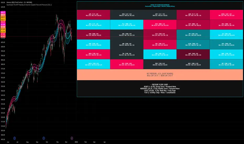
QuantLabs The MTF Nasdaq 30 Scanner [Capital Flow and Pressure]Trading the QQQ (Nasdaq) without knowing what the Generals (Apple, Nvidia, Microsoft) are doing is like driving at night with your headlights off. You might see the road right in front of you, but you'll miss the turn coming up.
The QuantLabs MTF Nasdaq 30 Scanner is not just a trend indicator, it is a professional-grade Market Dashboard that visualizes the heartbeat of the entire Nasdaq 100.
Why You Need This
Standard indicators lag. They tell you what happened after the move. This Heatmap tracks the Real-Time Capital Flow of the Top 30 companies that actually move the index ($Trillions in Market Cap).
Key Features
1. The "Spectacular" Precision Heatmap
Organized by Market Cap Size (AAPL/NVDA first).
Instantly spot divergent behavior. Is the market rallying, or is it just Nvidia holding everything up? The Heatmap reveals the truth instantly.
Colors: Neon Cyan (Bullish) vs Hot Pink (Bearish).
2. Triple Spectrum Technology (3-in-1 Timeframes) Why look at one timeframe when you can see three? Every cell in the dashboard displays the trend distance for:
8h (Fast): For scalping entries.
16h (Mid): For swing trends.
24h (Slow): For the major "Big Picture" bias.
Values denote % distance from the Flux Ribbon.
3. The "Net Pressure" Gauge (The Speedometer) A predictive summary footer that calculates the Weighted Pressure of the entire market.
HEAVY (> 0.5%): Strong Trend / Breakout Mode.
MODERATE (0.2% - 0.5%): Healthy, sustained move.
FLAT: Chop / Noise. Stay out.
It also shows exactly how much Capital ($Trillions) is sitting Bullish vs Bearish.
How to Trade with It
Check the "Net Pressure": If it says MODERATE BULLISH, you are looking for Longs only.
Scan the Top Row: Are the "Big 5" (AAPL, NVDA, MSFT...) aligned with the pressure?
Wait for Alignment: If the 8h, 16h, and 24h metrics all turn Cyan, that is a "Quantum Lock"—a high probability breakout signal.
Simple. Powerful. Neon. Add it to your chart and stop guessing the direction.
Credits: Built with 💜 by David James @ QuantLabs
Statistic
Strategy Validator - Backtest & Live TradeStrategy Validator is an analytical indicator for TradingView designed to evaluate trade setups, risk structure, and price behavior in real time.
The indicator builds trade scenarios, visualizes key trade levels, and provides statistical context based on historical data.
Its purpose is to help traders better understand current trade conditions and make decisions based on market structure rather than isolated signals.
🔶 Conceptual Approach
Many tools focus on a single question:
“Is there a signal right now?”
Strategy Validator approaches the market differently by analyzing a trade as a structured scenario that includes:
• current market state
• price position relative to key levels
• acceptable risk boundaries
• potential price expansion range
The indicator evaluates how well the active trade configuration aligns with historically observed market conditions and visualizes its boundaries directly on the chart.
🔶 Trade Condition Analysis
For each active configuration, the indicator evaluates:
• alignment of the entry with market structure
• market phase (directional movement, range, or elevated activity)
• risk-to-outcome relationship
• historical behavior of similar setups
The goal is to highlight trades with a clear structure and controlled risk , while filtering out weak or unstable conditions.
🎯 Trade Structure on Chart
Each trade is displayed directly on the chart with clearly defined elements:
• Entry — trade entry level
• Take Profit — projected target level
• Stop Loss — risk limitation level based on market structure and volatility
This allows immediate understanding of trade boundaries without manual calculations.
🧪 Statistical Context & Backtest
The indicator includes an integrated statistical panel showing:
• Win Rate
• Profit Factor
• Maximum Drawdown
• Net Result
• Total Trades
Two information blocks are available:
• BACKTEST — historical behavior of similar trade conditions
• POSITION — parameters and real-time state of the current trade
Historical data is used to provide analytical context, not to predict future performance.
🔶 Markets & Timeframes
🌍 Compatible with all TradingView markets:
• Crypto
• Forex
• Stocks & ETFs
• Indices
• Commodities
• Futures
⏱ Works on all timeframes — from intraday analysis to long-term charts.
🔶 Intended Use
Strategy Validator is designed for traders who:
• focus on risk-aware decision making
• prefer structured market analysis
• evaluate trades in context rather than isolation
• use statistics as a supporting decision layer
Important Notice
This indicator is an analytical tool and does not guarantee profitability.
It is not a trading robot or an automated execution system.
Past results do not guarantee future outcomes.
Always apply proper risk management.

Strategy Validator PRO - Backtest & Alerts📊 Strategy Validator PRO is a professional analytical indicator for TradingView designed to evaluate trade configurations, risk structure, and potential outcomes under current market conditions.
The indicator generates trade signals, visualizes entry and exit levels, and provides statistical context to support data-driven trading decisions rather than assumptions.
⚠️ PRO version is available by invitation only.
A simplified FREE version is publicly available for concept evaluation.
🔶 Core Concept
Most indicators answer the question:
“Where to enter?”
Strategy Validator PRO focuses on a more important one:
“How justified is this trade under current market conditions?”
The indicator applies a predefined analytical logic and evaluates how well the current trade setup aligns with statistically stable market conditions identified on an extended historical dataset.
🔶 Key Features
📈 Trade Configuration Analysis
The indicator evaluates:
• signal quality
• current market regime (trend, consolidation, volatility)
• risk-to-outcome structure
• historical behavior of similar setups
🎯 The goal is to filter weak or unfavorable trade conditions rather than simply generate signals.
🎯 Trade Structure on Chart
Each trade is displayed directly on the chart with a clear structure:
• Entry — trade entry level
• Take Profit — projected target level
• Stop Loss — risk limitation level based on market structure and volatility
This allows immediate understanding of trade boundaries without manual calculations.
🧪 Integrated Backtest Dashboard
The indicator displays performance statistics for the active logic:
• Win Rate
• Profit Factor
• Maximum Drawdown
• Net Profit
• Total Trades
Two panels are available:
• BACKTEST — historical performance overview
• POSITION — details of the current open trade
📌 Historical data is used to provide statistical context, not to predict future performance.
🔔 TradingView Alerts (PRO)
In the PRO version, alerts can be configured using TradingView’s native alert system.
Alerts may be created for:
• trade configuration formation
• target level reached
• risk limitation triggered
Available alert formats:
• Simple — plain text
• With levels — including price levels
• JSON — structured format for external analysis
🔶 PRO vs FREE
🟢 FREE
• Base analytical logic
• Limited historical depth
• Core trade structure
• Backtest dashboard
• Trade history
🔵 PRO
• Extended historical analysis
• Higher statistical sampling depth
• Trade condition filtering
• TradingView alerts
FREE version is intended for concept evaluation.
PRO version is designed for systematic and disciplined trading.
🔶 Markets & Timeframes
🌍 Compatible with all TradingView markets:
• Crypto
• Forex
• Stocks & ETFs
• Indices
• Commodities
• Futures
⏱ Works on all timeframes — from intraday to long-term.
🔶 Access
🔓 FREE version
Publicly available.
🔐 PRO version
Available by invitation.
Access can be requested via the author’s profile links or by contacting the author directly.
⚠️ Important Notice
This indicator is an analytical tool and does not guarantee profitability.
It is not a trading robot or automated execution system.
Past performance does not guarantee future results.
Always apply proper risk management.

Market Session Terrain Monitor vs 1.0 (UTC)Summary
Market Session Terrain Monitor helps traders understand where the market is within its normal intraday behavior, not where it should go. It is a decision-support tool designed to reduce late entries, over-trading, and narrative bias by grounding intraday analysis in historical session statistics.
Purpose
Market Session Terrain Monitor provides statistical context for intraday market movement by analyzing how much each major trading session typically moves, how much it has moved so far, and what market state the current session inherits from previous sessions.
The indicator is designed to answer one core question:
Is the current session early, normal, or already expanded relative to its historical behavior?
This indicator does not predict direction and does not generate buy or sell signals. It is intended as a context and state-awareness tool to support independent, structure-based decision making.
Sessions Analyzed
The trading day is divided into three independent sessions, defined in UTC time:
• Asia
• London
• New York
Each session is analyzed separately using its own historical data. No session is assumed to control or predict the behavior of another.
Session Range
For each session, the indicator measures the session range, defined as the session high minus the session low. This captures how much the market actually moved during that session, regardless of direction.
P90 Expansion Benchmark
For each session, the indicator calculates a P90 expansion benchmark.
• P90 represents the range that only about ten percent of historical sessions exceed
• It reflects a large but repeatable expansion, not an extreme outlier
• It is used as a normalization reference so sessions with different volatility characteristics can be compared on equal terms
The P90 values are displayed in the table header in price units, such as USD, as a reference for scale.
Percent of P90
Current and previous session ranges are expressed as a percentage of that session’s own P90.
This shows:
• How much of a statistically large session has already been used
• Whether the session is still early, behaving normally, or approaching expansion
Rolling Comparative Table
The table displays three rows, ordered by time and anchored to the current active session:
• Current · Session
• Previous · Session
• Previous-2 · Session
Each row shows:
• Session name
• Session range in price units
• Session range as a percentage of that session’s P90
This rolling layout provides context about the market state inherited by the current session without implying causality.
How to Use the Indicator
The indicator helps with:
• Identifying whether a session is early or late in its statistical range
• Avoiding entries when a session is already stretched
• Recognizing compression versus expansion regimes
• Understanding the market state the current session inherits
The indicator does not:
• Predict direction
• Forecast highs or lows
• Assume that one session determines the next
Directional decisions should come from price structure, execution rules, and risk management.
Design Philosophy
• Range first, direction second
• State awareness over narrative
• Statistical normalization instead of absolute numbers
• Comparative, not predictive
The indicator intentionally avoids estimating remaining range or subtracting previous session movement, as those approaches introduce bias and false causality.
Suitable Markets
• Gold and silver
• Forex pairs
• Indices
• Other liquid instruments with clear session behavior

Market Session Terrain Monitor v1.0Summary
Market Session Terrain Monitor helps traders understand where the market is within its normal intraday behavior, not where it should go. It is a decision-support tool designed to reduce late entries, over-trading, and narrative bias by grounding intraday analysis in historical session statistics.
Purpose
Market Session Terrain Monitor provides statistical context for intraday market movement by analyzing how much each major trading session typically moves, how much it has moved so far, and what market state the current session inherits from previous sessions.
The indicator is designed to answer one core question:
Is the current session early, normal, or already expanded relative to its historical behavior?
This indicator does not predict direction and does not generate buy or sell signals. It is intended as a context and state-awareness tool to support independent, structure-based decision making.
Sessions Analyzed
The trading day is divided into three independent sessions, defined in UTC time:
• Asia
• London
• New York
Each session is analyzed separately using its own historical data. No session is assumed to control or predict the behavior of another.
Session Range
For each session, the indicator measures the session range, defined as the session high minus the session low. This captures how much the market actually moved during that session, regardless of direction.
P90 Expansion Benchmark
For each session, the indicator calculates a P90 expansion benchmark.
• P90 represents the range that only about ten percent of historical sessions exceed
• It reflects a large but repeatable expansion, not an extreme outlier
• It is used as a normalization reference so sessions with different volatility characteristics can be compared on equal terms
The P90 values are displayed in the table header in price units, such as USD, as a reference for scale.
Percent of P90
Current and previous session ranges are expressed as a percentage of that session’s own P90.
This shows:
• How much of a statistically large session has already been used
• Whether the session is still early, behaving normally, or approaching expansion
Rolling Comparative Table
The table displays three rows, ordered by time and anchored to the current active session:
• Current · Session
• Previous · Session
• Previous-2 · Session
Each row shows:
• Session name
• Session range in price units
• Session range as a percentage of that session’s P90
This rolling layout provides context about the market state inherited by the current session without implying causality.
How to Use the Indicator
The indicator helps with:
• Identifying whether a session is early or late in its statistical range
• Avoiding entries when a session is already stretched
• Recognizing compression versus expansion regimes
• Understanding the market state the current session inherits
The indicator does not:
• Predict direction
• Forecast highs or lows
• Assume that one session determines the next
Directional decisions should come from price structure, execution rules, and risk management.
Design Philosophy
• Range first, direction second
• State awareness over narrative
• Statistical normalization instead of absolute numbers
• Comparative, not predictive
The indicator intentionally avoids estimating remaining range or subtracting previous session movement, as those approaches introduce bias and false causality.
Suitable Markets
• Gold and silver
• Forex pairs
• Indices
• Other liquid instruments with clear session behavior

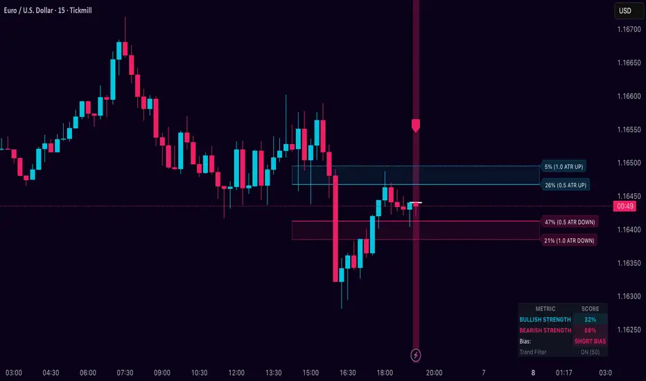
Dynamic Breakout Odds [RayAlgo]█ OVERVIEW
Dynamic Breakout Odds is a probability-based breakout tool that uses ATR and pattern matching to estimate how likely price is to expand up or down from the current candle.
Instead of guessing, the indicator scans historical candles that look like the current one and measures how often price broke above or below by a volatility-based amount.
It then projects those probabilities forward as clean levels and a bias dashboard on your chart.
Use it to quickly answer:
• “Is the next move statistically more likely up or down?”
• “How far does price typically travel from here, in ATR terms?”
█ CONCEPTS
Candle Profile Matching
The script builds a “profile” of the current setup using two elements:
• The color of the previous candle (bullish close vs bearish close)
• The trend environment (above/below EMA, if the filter is enabled)
Only historical candles with the same profile are used for statistics. This keeps the probabilities specific to the current context instead of mixing all market conditions together.
ATR-Based Expansion
For every matching historical candle, the script checks how far price moved away from the open using ATR:
• Upward move thresholds
• Moderate expansion (≈ 0.5 ATR above the open)
• Stronger expansion (≈ 1.0 ATR above the open)
• Downward move thresholds
• Moderate expansion (≈ 0.5 ATR below the open)
• Stronger expansion (≈ 1.0 ATR below the open)
It counts how often each expansion happened, then converts those counts into probabilities.
Normalized Probability Scores
The indicator doesn’t just show raw percentages; it normalizes them so that all scenarios together form a consistent probability set.
Internally it tracks four outcomes for similar candles:
• Chance of a moderate move upward
• Chance of a strong move upward
• Chance of a moderate move downward
• Chance of a strong move downward
These are then normalized so the total is roughly 100%. From this, two main metrics are derived:
• Bullish Strength = combined normalized odds of upside moves
• Bearish Strength = combined normalized odds of downside moves
Whichever side has the higher score defines the current directional bias .
█ WHAT YOU SEE ON THE CHART
1. Breakout Projection Levels
Four horizontal levels are projected around the open of the current bar:
• Two upside levels
• Nearer upside expansion (~0.5 ATR above the open)
• Further upside expansion (~1.0 ATR above the open)
• Two downside levels
• Nearer downside expansion (~0.5 ATR below the open)
• Further downside expansion (~1.0 ATR below the open)
Each line extends a configurable number of bars into the future, so you visually see a breakout “corridor” above and below price.
2. Probability Labels
At the right edge of each line, you’ll see a label such as:
• “X% – near upside”
• “Y% – further downside”
These labels tell you how frequently similar candles in the chosen lookback reached that expansion. You immediately know which scenario has been more common historically.
3. Breakout Zones
Between the paired upside lines and the paired downside lines, shaded “probability zones” can be shown:
• The upper shaded band highlights the typical upside expansion range
• The lower shaded band highlights the typical downside expansion range
These zones visually group probable target areas instead of just single lines.
4. Background Tint
The background behind price is softly tinted towards:
• Bullish color when Bullish Strength > Bearish Strength
• Bearish color when Bearish Strength > Bullish Strength
The stronger the statistical imbalance between the two, the more pronounced the tint. This gives you an instant feel for whether conditions lean more Long, more Short, or are nearly Neutral.
5. Directional Bias Arrow
On the last bar the script can plot a clean arrow:
• Up-arrow below price when bullish odds dominate
• Down-arrow above price when bearish odds dominate
The arrow is positioned beyond all projection lines, making it easy to see even on cluttered charts and reminding you of the current statistical bias without text.
6. Origin Marker
A small horizontal mark is drawn at the open of the current candle.
This acts as the “starting point” from which all ATR-based expansions above and below are measured.
7. Dashboard Panel
A compact dashboard is drawn in a corner of the chart (location configurable). It displays:
• Bullish Strength – combined normalized probability for upside expansions
• Bearish Strength – combined normalized probability for downside expansions
• Bias – “Long Bias”, “Short Bias”, or “Neutral”
• Trend Filter – shows whether EMA-based filtering is ON or OFF and which length is used
This gives you a quick, text-based summary of the current statistical environment.
█ SETTINGS
Analysis Lookback Period
• Controls how many historical bars the script inspects when searching for similar candles.
• Larger values = more history, smoother statistics, slower adaptation.
• Smaller values = faster adaptation, but more noise and less stability.
ATR Length
• The period used to compute ATR volatility.
• Defines how “big” 0.5 ATR and 1.0 ATR moves are on your current symbol and timeframe.
Trend Filter (EMA)
• Filter by Trend?
• When ON, only historical candles in a similar trend regime are used.
• When OFF, all past candles with similar color are considered, regardless of trend.
• Trend EMA Length
• EMA period used to classify trend.
• Price above EMA → uptrend environment.
• Price below EMA → downtrend environment.
This filter helps you separate behavior in uptrends from downtrends, which can significantly change breakout dynamics.
Visual Settings
• Projection Width (bars)
• How far the lines and zones extend into the future.
• Show Probability Zones
• Toggle shaded bands between each pair of levels.
• Label Size
• Choose smaller or larger text for the probability labels on the right.
• Tint Background by Bias
• Turn the bias-based background on or off.
• Show Bias Marker on Last Candle
• Toggle the up/down arrow marker.
• Dashboard Location
• Select top/bottom left/right corner for the panel.
█ HOW TO USE IT
1. Start With the Dashboard
Look at Bullish Strength vs Bearish Strength:
• If bullish is clearly larger → environment statistically favors upside expansion.
• If bearish is clearly larger → environment statistically favors downside expansion.
• If they are close → treat the situation as Neutral; consider reducing position size or waiting for more clarity.
2. Use Levels as Dynamic Targets
The projected lines and zones can serve as:
• Profit targets based on typical expansion distance
• Logical regions for scaling out
• Areas where you expect price behavior to change (e.g., loss of momentum)
Short-term traders often focus on the nearer expansion levels, while swing traders may use the farther levels as extended targets.
3. Align With Trend (Optional)
With the trend filter ON:
• Prefer Long setups when price is above the EMA and bullish probabilities dominate.
• Prefer Short setups when price is below the EMA and bearish probabilities dominate.
With the filter OFF, you get pure color-plus-pattern statistics across the whole lookback, which can be useful if you deliberately trade counter-trend or range conditions.
4. Combine With Your Existing System
Dynamic Breakout Odds is best used as a confirmation and targeting layer :
• Combine it with structure (support/resistance, supply/demand, order blocks).
• Combine it with volume or orderflow tools if you use them.
• Use the probability zones to validate whether your planned target is realistic relative to recent volatility.
It is not designed to be a standalone “buy/sell” signal generator, but a statistical map around your entries.
█ PRACTICAL EXAMPLES
Example A – Bullish, Moderate Expansion Frequently Hit
• Bullish Strength significantly higher than Bearish Strength.
• The nearer upside level shows a strong historical hit rate.
Interpretation: similar setups often produce at least a moderate push upward before failing.
Use case: trade pullbacks in the direction of the bias, targeting the nearer upside projection as an initial take-profit.
Example B – Bearish, Deeper Downside Often Reached
• Bearish Strength clearly dominant.
• Both the nearer and farther downside levels show decent probabilities.
Interpretation: similar conditions historically saw follow-through to the downside.
Use case: use rallies against the direction of the bias to position into shorts, planning partial exits around the first downside projection and runners toward the second.
Example C – Neutral, Balanced Probabilities
• Bullish and Bearish Strength scores are close.
• Background tint is very light or absent.
Interpretation: the market is statistically indecisive; expansions up or down are similarly likely.
Use case: consider range trading tactics, mean-reversion ideas, or simply standing aside until a clearer skew develops.
█ BEST PRACTICES
• Use on liquid symbols and reasonable timeframes to avoid distorted ATR behavior.
• Don’t overfit lookback length to a single instrument; test across markets.
• Let the indicator provide context, not absolute certainty.
• Always combine with proper risk management (position sizing, max loss per trade, etc.).
• Be cautious with very small sample sizes (e.g., very short lookbacks on low-volume assets).
█ LIMITATIONS & NOTES
• All probabilities are based on historical behavior ; markets can change regime.
• ATR distances are relative to recent volatility and may shrink/expand over time.
• The script intentionally does not guarantee any direction or target; it only reports what has been most common in similar past situations.
█ DISCLAIMER
This tool is for educational and informational purposes only.
It does not constitute financial advice or a guarantee of performance.
Always do your own research, test on demo or historical data, and use appropriate risk management when trading live capital.
Stock Relative Strength Rotation Graph🔄 Visualizing Market Rotation & Momentum (Stock RSRG)
This tool visualizes the sector rotation of your watchlist on a single graph. Instead of checking 40 different charts, you can see the entire market cycle in one view. It plots Relative Strength (Trend) vs. Momentum (Velocity) to identify which assets are leading the market and which are lagging.
📜 Credits & Disclaimer
Original Code: Adapted from the open-source " Relative Strength Scatter Plot " by LuxAlgo.
Trademark: This tool is inspired by Relative Rotation Graphs®. Relative Rotation Graphs® is a registered trademark of JOOS Holdings B.V. This script is neither endorsed, nor sponsored, nor affiliated with them.
📊 How It Works (The Math)
The script calculates two metrics for every symbol against a benchmark (Default: SPX):
X-Axis (RS-Ratio): Is the trend stronger than the benchmark? (>100 = Yes)
Y-Axis (RS-Momentum): Is the trend accelerating? (>100 = Yes)
🧩 The 4 Market Quadrants
🟩 Leading (Top-Right): Strong Trend + Accelerating. (Best for holding).
🟦 Improving (Top-Left): Weak Trend + Accelerating. (Best for entries).
⬜ Weakening (Bottom-Right): Strong Trend + Decelerating. (Watch for exits).
🟥 Lagging (Bottom-Left): Weak Trend + Decelerating. (Avoid).
✨ Significant Improvements
This open-source version adds unique features not found in standard rotation scripts:
📝 Quick-Input Engine: Paste up to 40 symbols as a single comma-separated list (e.g., NVDA, AMD, TSLA). No more individual input boxes.
🎯 Quadrant Filtering: You can now hide specific quadrants (like "Lagging") to clear the noise and focus only on actionable setups.
🐛 Trajectory Trails: Visualizes the historical path of the rotation so you can see the direction of momentum.
🛠️ How to Use
Paste Watchlist: Go to settings and paste your symbols (e.g., US Sectors: XLK, XLF, XLE...).
Find Entries: Look for tails moving from Improving ➔ Leading.
Find Exits: Be cautious when tails move from Leading ➔ Weakening.
Zoom: Use the "Scatter Plot Resolution" setting to zoom in or out if dots are bunched up.

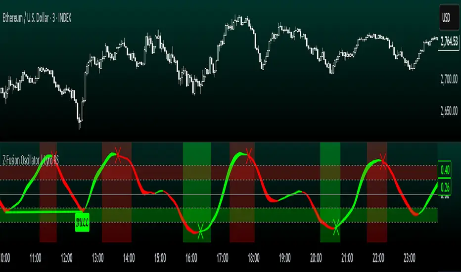
Z-Fusion Oscillator | Lyro RSThe Z-Fusion Oscillator converts five momentum indicators into Z-scores and blends them into one normalized signal that adapts across markets.
By combining normalization, smoothing, and divergence detection, users can easily identify when momentum is accelerating, weakening, reversing, or entering extreme zones
🔶 USAGE
The Z-Fusion Oscillator is designed to give traders a unified reading of market momentum—removing the noise of comparing tools that normally run on different scales.
By transforming RSI, MACD histogram, Stochastic, Momentum, and Rate of Change into Z-scores, this tool standardizes all inputs, making trend strength and shifts easier to interpret.
A dual-line system (fast Z-fusion line + slower baseline) highlights turning points, while overbought/oversold bands and “X-marks” help traders spot exhaustion and potential reversals.
🔹 Unified Momentum Structure
The indicator’s core strength comes from combining five Z-scored signals into one average.
Which makes momentum behavior more consistent across assets, reduces false extremes, and highlights true shifts in trend conviction.
🔹 Divergence Detection
The tool includes fully integrated divergence detection:
Regular Bullish Divergence: Price makes a lower low while Z-Fusion forms a higher low.
Regular Bearish Divergence: Price makes a higher high while Z-Fusion forms a lower high
Bullish and bearish divergences are marked directly on the oscillator with labels and colored pivot connections, making hidden momentum shifts obvious.
🔹 Visual Extremes
Two sets of upper and lower Z-score thresholds help identify:
Extreme overbought surges
Extreme oversold drops
Reversal zones
Potential exhaustion conditions
Background coloring reinforces when the oscillator moves beyond major levels, helping traders quickly assess momentum pressure.
🔹 Detecting Momentum Anomalies
Z-scores allow the oscillator to highlight when market momentum behaves abnormally relative to its own recent history.
For example:
The oscillator reaching +1 or –1 after an extended trend may indicate a climax.
A sharp Z-score reversal within an extreme zone can signal a trend exhaustion or a corrective move.
Divergences often appear earlier due to normalization smoothing out indicator noise.
This makes the Z-Fusion Oscillator particularly useful for spotting subtle shifts in trend direction that traditional indicators may miss.
🔶 DETAILS
🔹 Composite Z-Score Framework
Each momentum tool is smoothed, normalized, and transformed:
RSI → EMA-smoothed, Z-scored
MACD histogram → Z-scored
Stochastic → EMA + SMA smoothing, then Z-scored
Momentum → EMA-smoothed, Z-scored
Rate of Change → EMA-smoothed, Z-scored
These are averaged into one composite Z-score to provide a consistent reading across assets and market conditions.
🔹 Fusion Trend Lines
Two lines serve as the core signal:
Fast Line (savg) – reacts quicker to trend changes
Slow Line (savg2) – acts as a baseline filter
Crossovers between these lines highlight momentum shifts, while their color reflects trend bias.
🔹 Overbought/Oversold Zones
Two upper and two lower Z-score thresholds define “zones”:
Upper zones highlight overheated momentum or potential bearish reversals
Lower zones highlight depressed momentum or potential bullish reversals
Filled regions and background colors help visually confirm extreme conditions.
🔹 Pivot-Based Divergence Engine
The script includes filtered pivot detection with customizable look-backs and range limits to ensure divergences are meaningful, not noise-driven.
🔶 SETTINGS
🔹 Indicator Settings
Source — Price series used for all calculations.
Z-Score Length — Lookback period for Z-score normalization.
Z-Score MA Length — Smoothing length for the fusion signal lines.
Overbought/Oversold Levels — Four customizable threshold lines.
Color Palette — Choose from preset themes or define custom colors.
🔹 RSI
Length — RSI calculation period.
EMA Smoothing Length — Smooths RSI before Z-score conversion.
🔹 MACD
Fast Length — Fast EMA length.
Slow Length — Slow EMA length.
Signal Line Length — MACD signal smoothing.
🔹 Stochastic
%K Length — Main stochastic length.
EMA Smoothing — Smooths %K for stability.
%D Length — Smoothing for the signal line.
🔹 Momentum
Length — Momentum lookback.
EMA Smoothing — Smooths momentum before Z-scoring.
🔹 Rate of Change
Length — ROC lookback.
EMA Smoothing — Smooths ROC values.
🔹 Divergence
Enable/Disable Divergence Detection — Toggle divergence engine.
Pivot Left/Right Lookback — Defines pivot detection sensitivity.
Detection Range Limits — Controls allowable range for divergence.
Bull/Bear Colors & Styling — Customize divergence visualization.
🔶 SUMMARY
The Z-Fusion Oscillator combines multiple momentum signatures into a single normalized signal, enabling traders to:
Identify reversals early
Detect momentum exhaustion
Spot bullish and bearish divergences
Track overbought/oversold conditions
Visualize trend strength with clarity
Whether you're a swing trader, intraday analyst, or trend-reversal hunter, the Z-Fusion Oscillator provides a powerful and adaptive way to read momentum.
Multi-Asset % Performance Table | v2.1 | TCP Multi-Asset % Performance Table | v2.1 | TCP
ESSENTIAL SUMMARY:
Multi-Asset % Performance Table eliminates the need to manually draw and manage individual "Price Range" tools for every asset. It automatically tracks up to 15 tickers independently in a single dashboard, calculating a TOTAL SCORE (Portfolio Average) for you. Unlike manual drawings, it supports a Global Range while allowing Custom Dates for specific assets, ensuring each ticker is calculated based on its own precise entry/exit. The Smart Visuals dynamically draw the correct date lines only for the ticker you are currently viewing, keeping your chart automatic, accurate, and clutter-free.
FUL DESCRIPTION:
📊 What is this tool?
The Multi-Asset % Performance Table is a powerful portfolio dashboard designed to track the percentage performance of up to 15 different assets simultaneously.
Instead of checking tickers one by one or manually drawing price ranges, this indicator aggregates everything into a single, clean table. It allows you to compare the ROI (Return on Investment) of a basket of coins or stocks over a specific time period and calculates an aggregate TOTAL SCORE (Average %) for your selection.
🚀 Key Features
15 Asset Slots: Monitor up to 15 different tickers (Crypto, Stocks, Forex, etc.) in one view.
Global vs. Custom Dates: Set a "Global" start/end date for the whole portfolio, but override specific assets with Custom Dates if they entered the portfolio at a different time.
Smart Visuals: Automatically draws vertical dashed lines on your chart representing the start and end dates of the ticker you are currently viewing.
Total Score Calculation: Calculates the average percentage change of your portfolio. You can dynamically include or exclude specific assets from this average using the settings.
Status Column: A quick visual reference (✔ or ✘) in the table showing which assets are currently included in the Total Score calculation.
⚙️ How it Works
Data Fetching: The script pulls "Close" prices from the Daily timeframe to ensure accuracy across long periods.
Smart Matching: The visual lines automatically detect which asset you are viewing. For example, if you are looking at BTCUSDT and have custom dates set for it, the vertical lines will jump to those specific dates. If you view a ticker not in your list, it defaults to the Global dates.
Visual Protection: The script uses advanced logic to ensure only one set of range lines appears on the chart at a time, keeping your workspace clean.
🛠️ Instructions & Settings
1. Setting up your Assets
Open the Settings (Cogwheel icon).
Under ASSET 1 through ASSET 15, enter the tickers you want to track (e.g., BINANCE:BTCUSDT).
Include in Avg?: Uncheck this if you want to see the asset in the table but exclude it from the "TOTAL SCORE" average.
2. Defining Time Ranges
Global Settings: Set the Global Start and Global End dates at the top. This applies to all assets by default.
Custom Dates: If a specific asset (e.g., Asset 4) was bought on a different day, check the "Custom Dates?" box for that asset and enter its specific Start/End time.
3. Reading the Table
The table appears on the chart (default: Bottom Right) with three columns:
Asset: The name of the ticker.
% Change: The percentage move from Start Date to End Date. (Green = Positive, Red = Negative).
Inc: Shows a ✔ if the asset is included in the Total Score average, or a ✘ if excluded.
4. The Visual Lines
Two vertical dashed lines will appear on your chart.
Note: These lines are visual references only. You cannot drag them to change the dates. To change the dates, you must use the Settings menu.
💡 Tips
Hover for Details: Hover your mouse over the % Change value in the table to see a tooltip showing the exact Start Price and End Price used for the calculation.
Resolution: The script defaults to 1 Day resolution for optimal accuracy on historical data.
v2.1 | TCP - Custom Built for Precision Performance Tracking

Spot-Futures SpreadSpot-Futures Spread Indicator
A comprehensive indicator that automatically calculates and visualizes the percentage spread between spot and perpetual futures prices across multiple exchanges.
Key Features:
Automatic Exchange Detection - Automatically detects your current exchange and finds the corresponding spot/futures pair
Smart Fallback System - If the counterpart isn't available on your exchange, it automatically searches across 7+ major exchanges (Binance, Bybit, OKX, Gate.io, MEXC, KuCoin, HTX) and uses the first valid match
Multi-Exchange Support - Works with 14 exchanges including Binance, Bybit, OKX, MEXC, BitGet, Gate.io, KuCoin, and more
Clear Exchange Attribution - Shows exactly which exchanges are providing spot and futures data in the statistics table
Configurable Moving Average - Track the average spread with customizable period
Standard Deviation Bands - Identify unusual spread conditions with Bollinger-style bands
Built-in Alerts - Get notified when spread crosses bands or zero (parity)
Statistics Table - Real-time stats showing current spread, MA, std dev, and bands
Manual Override Options - Advanced users can manually specify exchanges and symbols
How It Works:
The indicator calculates the spread as: (Futures Price - Spot Price) / Spot Price × 100
Positive spread = Futures trading at a premium (contango)
Negative spread = Futures trading at a discount (backwardation)
Zero = Parity between spot and futures
Use Cases:
Funding Rate Analysis - Correlates with perpetual funding rates
Arbitrage Opportunities - Identify significant spot-futures divergences
Market Sentiment - Premium/discount indicates bullish/bearish positioning
Cross-Exchange Analysis - Compare spreads when spot and futures are on different exchanges
Smart Features:
Works whether you're viewing a spot or futures chart
Automatically handles exchange-specific perpetual contract naming (.P, PERP, SWAP, etc.)
Color-coded visualization (green for premium, red for discount)
Customizable colors and display options
Background shading based on spread direction
Perfect For:
Crypto traders monitoring funding rates, arbitrage traders, market makers, and anyone interested in spot-futures dynamics across multiple exchanges.
Getting Started:
Simply add the indicator to any spot or perpetual futures chart. It will automatically detect the exchange and find the corresponding pair. The statistics table shows which exchanges are being used for maximum transparency.
Note: The indicator automatically ignores invalid symbols, so you'll never see errors even if a specific pair doesn't exist on a particular exchange.
Kudos to @AlekMel that made the "Spot - Fut Spread v2" indicator that I enhance the Automatic detection feature which was not working in some case.

LibWghtLibrary "LibWght"
This is a library of mathematical and statistical functions
designed for quantitative analysis in Pine Script. Its core
principle is the integration of a custom weighting series
(e.g., volume) into a wide array of standard technical
analysis calculations.
Key Capabilities:
1. **Universal Weighting:** All exported functions accept a `weight`
parameter. This allows standard calculations (like moving
averages, RSI, and standard deviation) to be influenced by an
external data series, such as volume or tick count.
2. **Weighted Averages and Indicators:** Includes a comprehensive
collection of weighted functions:
- **Moving Averages:** `wSma`, `wEma`, `wWma`, `wRma` (Wilder's),
`wHma` (Hull), and `wLSma` (Least Squares / Linear Regression).
- **Oscillators & Ranges:** `wRsi`, `wAtr` (Average True Range),
`wTr` (True Range), and `wR` (High-Low Range).
3. **Volatility Decomposition:** Provides functions to decompose
total variance into distinct components for market analysis.
- **Two-Way Decomposition (`wTotVar`):** Separates variance into
**between-bar** (directional) and **within-bar** (noise)
components.
- **Three-Way Decomposition (`wLRTotVar`):** Decomposes variance
relative to a linear regression into **Trend** (explained by
the LR slope), **Residual** (mean-reversion around the
LR line), and **Within-Bar** (noise) components.
- **Local Volatility (`wLRLocTotStdDev`):** Measures the total
"noise" (within-bar + residual) around the trend line.
4. **Weighted Statistics and Regression:** Provides a robust
function for Weighted Linear Regression (`wLinReg`) and a
full suite of related statistical measures:
- **Between-Bar Stats:** `wBtwVar`, `wBtwStdDev`, `wBtwStdErr`.
- **Residual Stats:** `wResVar`, `wResStdDev`, `wResStdErr`.
5. **Fallback Mechanism:** All functions are designed for reliability.
If the total weight over the lookback period is zero (e.g., in
a no-volume period), the algorithms automatically fall back to
their unweighted, uniform-weight equivalents (e.g., `wSma`
becomes a standard `ta.sma`), preventing errors and ensuring
continuous calculation.
---
**DISCLAIMER**
This library is provided "AS IS" and for informational and
educational purposes only. It does not constitute financial,
investment, or trading advice.
The author assumes no liability for any errors, inaccuracies,
or omissions in the code. Using this library to build
trading indicators or strategies is entirely at your own risk.
As a developer using this library, you are solely responsible
for the rigorous testing, validation, and performance of any
scripts you create based on these functions. The author shall
not be held liable for any financial losses incurred directly
or indirectly from the use of this library or any scripts
derived from it.
wSma(source, weight, length)
Weighted Simple Moving Average (linear kernel).
Parameters:
source (float) : series float Data to average.
weight (float) : series float Weight series.
length (int) : series int Look-back length ≥ 1.
Returns: series float Linear-kernel weighted mean; falls back to
the arithmetic mean if Σweight = 0.
wEma(source, weight, length)
Weighted EMA (exponential kernel).
Parameters:
source (float) : series float Data to average.
weight (float) : series float Weight series.
length (simple int) : simple int Look-back length ≥ 1.
Returns: series float Exponential-kernel weighted mean; falls
back to classic EMA if Σweight = 0.
wWma(source, weight, length)
Weighted WMA (linear kernel).
Parameters:
source (float) : series float Data to average.
weight (float) : series float Weight series.
length (int) : series int Look-back length ≥ 1.
Returns: series float Linear-kernel weighted mean; falls back to
classic WMA if Σweight = 0.
wRma(source, weight, length)
Weighted RMA (Wilder kernel, α = 1/len).
Parameters:
source (float) : series float Data to average.
weight (float) : series float Weight series.
length (simple int) : simple int Look-back length ≥ 1.
Returns: series float Wilder-kernel weighted mean; falls back to
classic RMA if Σweight = 0.
wHma(source, weight, length)
Weighted HMA (linear kernel).
Parameters:
source (float) : series float Data to average.
weight (float) : series float Weight series.
length (int) : series int Look-back length ≥ 1.
Returns: series float Linear-kernel weighted mean; falls back to
classic HMA if Σweight = 0.
wRsi(source, weight, length)
Weighted Relative Strength Index.
Parameters:
source (float) : series float Price series.
weight (float) : series float Weight series.
length (simple int) : simple int Look-back length ≥ 1.
Returns: series float Weighted RSI; uniform if Σw = 0.
wAtr(tr, weight, length)
Weighted ATR (Average True Range).
Implemented as WRMA on *true range*.
Parameters:
tr (float) : series float True Range series.
weight (float) : series float Weight series.
length (simple int) : simple int Look-back length ≥ 1.
Returns: series float Weighted ATR; uniform weights if Σw = 0.
wTr(tr, weight, length)
Weighted True Range over a window.
Parameters:
tr (float) : series float True Range series.
weight (float) : series float Weight series.
length (int) : series int Look-back length ≥ 1.
Returns: series float Weighted mean of TR; uniform if Σw = 0.
wR(r, weight, length)
Weighted High-Low Range over a window.
Parameters:
r (float) : series float High-Low per bar.
weight (float) : series float Weight series.
length (int) : series int Look-back length ≥ 1.
Returns: series float Weighted mean of range; uniform if Σw = 0.
wBtwVar(source, weight, length, biased)
Weighted Between Variance (biased/unbiased).
Parameters:
source (float) : series float Data series.
weight (float) : series float Weight series.
length (int) : series int Look-back length ≥ 2.
biased (bool) : series bool true → population (biased); false → sample.
Returns:
variance series float The calculated between-bar variance (σ²btw), either biased or unbiased.
sumW series float The sum of weights over the lookback period (Σw).
sumW2 series float The sum of squared weights over the lookback period (Σw²).
wBtwStdDev(source, weight, length, biased)
Weighted Between Standard Deviation.
Parameters:
source (float) : series float Data series.
weight (float) : series float Weight series.
length (int) : series int Look-back length ≥ 2.
biased (bool) : series bool true → population (biased); false → sample.
Returns: series float σbtw uniform if Σw = 0.
wBtwStdErr(source, weight, length, biased)
Weighted Between Standard Error.
Parameters:
source (float) : series float Data series.
weight (float) : series float Weight series.
length (int) : series int Look-back length ≥ 2.
biased (bool) : series bool true → population (biased); false → sample.
Returns: series float √(σ²btw / N_eff) uniform if Σw = 0.
wTotVar(mu, sigma, weight, length, biased)
Weighted Total Variance (= between-group + within-group).
Useful when each bar represents an aggregate with its own
mean* and pre-estimated σ (e.g., second-level ranges inside a
1-minute bar). Assumes the *weight* series applies to both the
group means and their σ estimates.
Parameters:
mu (float) : series float Group means (e.g., HL2 of 1-second bars).
sigma (float) : series float Pre-estimated σ of each group (same basis).
weight (float) : series float Weight series (volume, ticks, …).
length (int) : series int Look-back length ≥ 2.
biased (bool) : series bool true → population (biased); false → sample.
Returns:
varBtw series float The between-bar variance component (σ²btw).
varWtn series float The within-bar variance component (σ²wtn).
sumW series float The sum of weights over the lookback period (Σw).
sumW2 series float The sum of squared weights over the lookback period (Σw²).
wTotStdDev(mu, sigma, weight, length, biased)
Weighted Total Standard Deviation.
Parameters:
mu (float) : series float Group means (e.g., HL2 of 1-second bars).
sigma (float) : series float Pre-estimated σ of each group (same basis).
weight (float) : series float Weight series (volume, ticks, …).
length (int) : series int Look-back length ≥ 2.
biased (bool) : series bool true → population (biased); false → sample.
Returns: series float σtot.
wTotStdErr(mu, sigma, weight, length, biased)
Weighted Total Standard Error.
SE = √( total variance / N_eff ) with the same effective sample
size logic as `wster()`.
Parameters:
mu (float) : series float Group means (e.g., HL2 of 1-second bars).
sigma (float) : series float Pre-estimated σ of each group (same basis).
weight (float) : series float Weight series (volume, ticks, …).
length (int) : series int Look-back length ≥ 2.
biased (bool) : series bool true → population (biased); false → sample.
Returns: series float √(σ²tot / N_eff).
wLinReg(source, weight, length)
Weighted Linear Regression.
Parameters:
source (float) : series float Data series.
weight (float) : series float Weight series.
length (int) : series int Look-back length ≥ 2.
Returns:
mid series float The estimated value of the regression line at the most recent bar.
slope series float The slope of the regression line.
intercept series float The intercept of the regression line.
wResVar(source, weight, midLine, slope, length, biased)
Weighted Residual Variance.
linear regression – optionally biased (population) or
unbiased (sample).
Parameters:
source (float) : series float Data series.
weight (float) : series float Weighting series (volume, etc.).
midLine (float) : series float Regression value at the last bar.
slope (float) : series float Slope per bar.
length (int) : series int Look-back length ≥ 2.
biased (bool) : series bool true → population variance (σ²_P), denominator ≈ N_eff.
false → sample variance (σ²_S), denominator ≈ N_eff - 2.
(Adjusts for 2 degrees of freedom lost to the regression).
Returns:
variance series float The calculated residual variance (σ²res), either biased or unbiased.
sumW series float The sum of weights over the lookback period (Σw).
sumW2 series float The sum of squared weights over the lookback period (Σw²).
wResStdDev(source, weight, midLine, slope, length, biased)
Weighted Residual Standard Deviation.
Parameters:
source (float) : series float Data series.
weight (float) : series float Weight series.
midLine (float) : series float Regression value at the last bar.
slope (float) : series float Slope per bar.
length (int) : series int Look-back length ≥ 2.
biased (bool) : series bool true → population (biased); false → sample.
Returns: series float σres; uniform if Σw = 0.
wResStdErr(source, weight, midLine, slope, length, biased)
Weighted Residual Standard Error.
Parameters:
source (float) : series float Data series.
weight (float) : series float Weight series.
midLine (float) : series float Regression value at the last bar.
slope (float) : series float Slope per bar.
length (int) : series int Look-back length ≥ 2.
biased (bool) : series bool true → population (biased); false → sample.
Returns: series float √(σ²res / N_eff); uniform if Σw = 0.
wLRTotVar(mu, sigma, weight, midLine, slope, length, biased)
Weighted Linear-Regression Total Variance **around the
window’s weighted mean μ**.
σ²_tot = E_w ⟶ *within-group variance*
+ Var_w ⟶ *residual variance*
+ Var_w ⟶ *trend variance*
where each bar i in the look-back window contributes
m_i = *mean* (e.g. 1-sec HL2)
σ_i = *sigma* (pre-estimated intrabar σ)
w_i = *weight* (volume, ticks, …)
ŷ_i = b₀ + b₁·x (value of the weighted LR line)
r_i = m_i − ŷ_i (orthogonal residual)
Parameters:
mu (float) : series float Per-bar mean m_i.
sigma (float) : series float Pre-estimated σ_i of each bar.
weight (float) : series float Weight series w_i (≥ 0).
midLine (float) : series float Regression value at the latest bar (ŷₙ₋₁).
slope (float) : series float Slope b₁ of the regression line.
length (int) : series int Look-back length ≥ 2.
biased (bool) : series bool true → population; false → sample.
Returns:
varRes series float The residual variance component (σ²res).
varWtn series float The within-bar variance component (σ²wtn).
varTrd series float The trend variance component (σ²trd), explained by the linear regression.
sumW series float The sum of weights over the lookback period (Σw).
sumW2 series float The sum of squared weights over the lookback period (Σw²).
wLRTotStdDev(mu, sigma, weight, midLine, slope, length, biased)
Weighted Linear-Regression Total Standard Deviation.
Parameters:
mu (float) : series float Per-bar mean m_i.
sigma (float) : series float Pre-estimated σ_i of each bar.
weight (float) : series float Weight series w_i (≥ 0).
midLine (float) : series float Regression value at the latest bar (ŷₙ₋₁).
slope (float) : series float Slope b₁ of the regression line.
length (int) : series int Look-back length ≥ 2.
biased (bool) : series bool true → population; false → sample.
Returns: series float √(σ²tot).
wLRTotStdErr(mu, sigma, weight, midLine, slope, length, biased)
Weighted Linear-Regression Total Standard Error.
SE = √( σ²_tot / N_eff ) with N_eff = Σw² / Σw² (like in wster()).
Parameters:
mu (float) : series float Per-bar mean m_i.
sigma (float) : series float Pre-estimated σ_i of each bar.
weight (float) : series float Weight series w_i (≥ 0).
midLine (float) : series float Regression value at the latest bar (ŷₙ₋₁).
slope (float) : series float Slope b₁ of the regression line.
length (int) : series int Look-back length ≥ 2.
biased (bool) : series bool true → population; false → sample.
Returns: series float √((σ²res, σ²wtn, σ²trd) / N_eff).
wLRLocTotStdDev(mu, sigma, weight, midLine, slope, length, biased)
Weighted Linear-Regression Local Total Standard Deviation.
Measures the total "noise" (within-bar + residual) around the trend.
Parameters:
mu (float) : series float Per-bar mean m_i.
sigma (float) : series float Pre-estimated σ_i of each bar.
weight (float) : series float Weight series w_i (≥ 0).
midLine (float) : series float Regression value at the latest bar (ŷₙ₋₁).
slope (float) : series float Slope b₁ of the regression line.
length (int) : series int Look-back length ≥ 2.
biased (bool) : series bool true → population; false → sample.
Returns: series float √(σ²wtn + σ²res).
wLRLocTotStdErr(mu, sigma, weight, midLine, slope, length, biased)
Weighted Linear-Regression Local Total Standard Error.
Parameters:
mu (float) : series float Per-bar mean m_i.
sigma (float) : series float Pre-estimated σ_i of each bar.
weight (float) : series float Weight series w_i (≥ 0).
midLine (float) : series float Regression value at the latest bar (ŷₙ₋₁).
slope (float) : series float Slope b₁ of the regression line.
length (int) : series int Look-back length ≥ 2.
biased (bool) : series bool true → population; false → sample.
Returns: series float √((σ²wtn + σ²res) / N_eff).
wLSma(source, weight, length)
Weighted Least Square Moving Average.
Parameters:
source (float) : series float Data series.
weight (float) : series float Weight series.
length (int) : series int Look-back length ≥ 2.
Returns: series float Least square weighted mean. Falls back
to unweighted regression if Σw = 0.
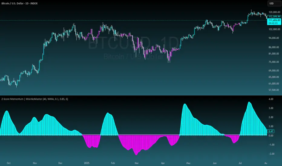
Z-Score Momentum | MisinkoMasterThe Z-Score Momentum is a new trend analysis indicator designed to catch reversals, and shifts in trends by comparing the "positive" and "negative" momentum by using the Z-Score.
This approach helps traders and investors get unique insight into the market of not just Crypto, but any market.
A deeper dive into the indicator
First, I want to cover the "Why?", as I believe it will ease of the part of the calculation to make it easier to understand, as by then you will understand how it fits the puzzle.
I had an attempt to create a momentum oscillator that would catch reversals and provide high tier accuracy while maintaining the main part => the speed.
I thought back to many concepts, divergences between averages?
- Did not work
Maybe a MACD rework?
- Did not work with what I tried :(
So I thought about statistics, Standard Deviation, Z-Score, Sharpe/Sortino/Omega ratio...
Wait, was that the Z-Score? I only tried the For Loop version of it :O
So on my way back from school I formulated a concept (originaly not like this but to that later) that would attempt to use the Z-Score as an accurate momentum oscillator.
Many ideas were falling out of the blue, but not many worked.
After almost giving up on this, and going to go back to developing my strategies, I tried one last thing:
What if we use divergences in the average, formulated like a Z-score?
Surprise-surprise, it worked!
Now to explain what I have been so passionately yapping about, and to connect the pieces of the puzzle once and for all:
The indicator compares the "strength" of the bullish/bearish factors (could be said differently, but this is my "speach bubble", and I think this describes it the best)
What could we use for the "bullish/bearish" factors?
How about high & low?
I mean, these are by definitions the highest and lowest points in price, which I decided to interpret as: The highest the bull & bear "factors" achieved that bar.
The problem here is comparison, I mean high will ALWAYS > low, unless the asset decided to unplug itself and stop moving, but otherwise that would be unfair.
Now if I use my Z-score, it will get higher while low is going up, which is the opposite of what I want, the bearish "factor" is weaker while we go up!
So I sat on my ret*rded a*s for 25 minutes, completly ignoring the fact the number "-1" exists.
Surprise surprise, multiplying the Z-Score of the low by -1 did what I wanted!
Now it reversed itself (magically). Now while the low keeps going down, the bear factor increases, and while it goes up the bear factor lowers.
This was btw still too noisy, so instead of the classic formula:
a = current value
b = average value
c = standard deviation of a
Z = (a-b)/c
I used:
a = average value over n/2 period
b = average value over n period
c = standard deviation of a
Z = (a-b)/c
And then compared the Z-Score of High to the Z-Score of Low by basic subtraction, which gives us final result and shows us the strength of trend, the direction of the trend, and possibly more, which I may have not found.
As always, this script is open source, so make sure to play around with it, you may uncover the treasure that I did not :)
Enjoy Gs!
Trade-o-Scope: Plot Custom Data v2Meet — a major tool upgrade for plotting your own data on TradingView charts. Simple and intuitive input format, large volume limits, and robust plotting for your own datasets — forecasts, backtests, or external data and model outputs.
You can apply/overlay other indicators from the TradingView catalog (such as Bollinger Bands, RSI, etc.) on top of custom data charts. The indicator you want to overlay must support selecting an input data source — i.e., have a dropdown where you can choose as the source.
🧩 How to use
Simply select and copy two columns — with dates and values — from your spreadsheet (Excel, Google Sheets, etc.) and paste them into the indicator’s input field. The indicator will automatically process the input and plot your data on the chart.
Example data:
Date XYZ_value
2025-10-08 84.57
2025-10-01 80.66
2025-09-24 86.24
2025-09-17 84.76
📅 Supported date format
The indicator recognizes standard international date formats commonly used in spreadsheets and data exports.
• ISO 8601 — "YYYY-MM-DD" or "YYYY-MM-DDThh:mm:ss"
2025-10-13
2025-10-13 14:30
2025-10-13 14:30:00
2025-10-13T14:30
2025-10-13T14:30:00
• RFC 2822 — "DD MMM YYYY" or "DD MMM YYYY hh:mm:ss"
13 Oct 2025
13 Oct 2025 14:30
13 Oct 2025 14:30:00
The time part is optional — if omitted, midnight (00:00:00) is assumed.
By default, all date–time values are interpreted in the exchange timezone of the chart’s symbol, but you can select a different data timezone in the indicator settings if needed.
💡 Supported value format
Integers (e.g., 12345, -12345)
Decimals (e.g., 1234.56, -1234.56)
The decimal separator must be a dot (.)
Thousands separators are not supported
⚙️ Advanced Features
Value Multiplier — scale your values by a chosen factor.
Formatting Options — display values as price, percentage, or volume.
Conditional Coloring — automatically change plot color based on thresholds.
Plot Style Selection — choose from line, histogram, area, or column plots.
Additional Visual References — enable fixed horizontal lines for better visual interpretation.
📝 General Notes
Maximum input size: 40,960 characters (~1,500–3,000 rows depending on format). If an error occurs after pasting data, simply remove a few rows until it disappears.

First Passage Time - Distribution AnalysisThe First Passage Time (FPT) Distribution Analysis indicator is a sophisticated probabilistic tool that answers one of the most critical questions in trading: "How long will it take for price to reach my target, and what are the odds of getting there first?"
Unlike traditional technical indicators that focus on what might happen, this indicator tells you when it's likely to happen.
Mathematical Foundation: First Passage Time Theory
What is First Passage Time?
First Passage Time (FPT) is a concept in stochastic processes that measures the time it takes for a random process to reach a specific threshold for the first time. Originally developed in physics and mathematics, FPT has applications in:
Quantitative Finance: Option pricing, risk management, and algorithmic trading
Neuroscience: Modeling neural firing patterns
Biology: Population dynamics and disease spread
Engineering: Reliability analysis and failure prediction
The Mathematics Behind It
This indicator uses Geometric Brownian Motion (GBM), the same stochastic model used in the Black-Scholes option pricing formula:
dS = μS dt + σS dW
Where:
S = Asset price
μ = Drift (trend component)
σ = Volatility (uncertainty component)
dW = Wiener process (random walk)
Through Monte Carlo simulation, the indicator runs 1,000+ price path simulations to statistically determine:
When each threshold (+X% or -X%) is likely to be hit
Which threshold is hit first (directional bias)
How often each scenario occurs (probability distribution)
🎯 How This Indicator Works
Core Algorithm Workflow:
Calculate Historical Statistics
Measures recent price volatility (standard deviation of log returns)
Calculates drift (average directional movement)
Annualizes these metrics for meaningful comparison
Run Monte Carlo Simulations
Generates 1,000+ random price paths based on historical behavior
Tracks when each path hits the upside (+X%) or downside (-X%) threshold
Records which threshold was hit first in each simulation
Aggregate Statistical Results
Calculates percentile distributions (10th, 25th, 50th, 75th, 90th)
Computes "first hit" probabilities (upside vs downside)
Determines average and median time-to-target
Visual Representation
Displays thresholds as horizontal lines
Shows gradient risk zones (purple-to-blue)
Provides comprehensive statistics table
📈 Use Cases
1. Options Trading
Selling Options: Determine if your strike price is likely to be hit before expiration
Buying Options: Estimate probability of reaching profit targets within your time window
Time Decay Management: Compare expected time-to-target vs theta decay
Example: You're considering selling a 30-day call option 5% out of the money. The indicator shows there's a 72% chance price hits +5% within 12 days. This tells you the trade has high assignment risk.
2. Swing Trading
Entry Timing: Wait for higher probability setups when directional bias is strong
Target Setting: Use median time-to-target to set realistic profit expectations
Stop Loss Placement: Understand probability of hitting your stop before target
Example: The indicator shows 85% upside probability with median time of 3.2 days. You can confidently enter long positions with appropriate position sizing.
3. Risk Management
Position Sizing: Larger positions when probability heavily favors one direction
Portfolio Allocation: Reduce exposure when probabilities are near 50/50 (high uncertainty)
Hedge Timing: Know when to add protective positions based on downside probability
Example: Indicator shows 55% upside vs 45% downside—nearly neutral. This signals high uncertainty, suggesting reduced position size or wait for better setup.
4. Market Regime Detection
Trending Markets: High directional bias (70%+ one direction)
Range-bound Markets: Balanced probabilities (45-55% both directions)
Volatility Regimes: Compare actual vs theoretical minimum time
Example: Consistent 90%+ bullish bias across multiple timeframes confirms strong uptrend—stay long and avoid counter-trend trades.
First Hit Rate (Most Important!)
Shows which threshold is likely to be hit FIRST:
Upside %: Probability of hitting upside target before downside
Downside %: Probability of hitting downside target before upside
These always sum to 100%
⚠️ Warning: If you see "Low Hit Rate" warning, increase this parameter!
Advanced Parameters
Drift Mode
Allows you to explore different scenarios:
Historical: Uses actual recent trend (default—most realistic)
Zero (Neutral): Assumes no trend, only volatility (symmetric probabilities)
50% Reduced: Dampens trend effect (conservative scenario)
Use Case: Switch to "Zero (Neutral)" to see what happens in a pure volatility environment, useful for range-bound markets.
Distribution Type
Percentile: Shows 10%, 25%, 50%, 75%, 90% levels (recommended for most users)
Sigma: Shows standard deviation levels (1σ, 2σ)—useful for statistical analysis
⚠️ Important Limitations & Best Practices
Limitations
Assumes GBM: Real markets have fat tails, jumps, and regime changes not captured by GBM
Historical Parameters: Uses recent volatility/drift—may not predict regime shifts
No Fundamental Events: Cannot predict earnings, news, or macro shocks
Computational: Runs only on last bar—doesn't give historical signals
Remember: Probabilities are not certainties. Use this indicator as part of a comprehensive trading plan with proper risk management.
Created by: Henrique Centieiro. feedback is more than welcome!

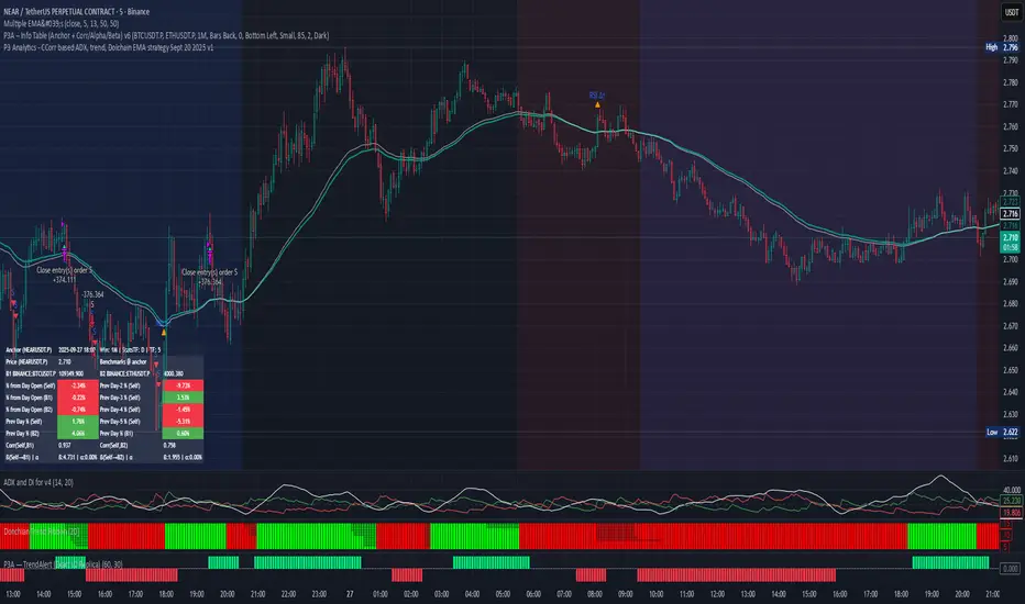
PPP – Info Table (Anchor + Corr/Alpha/Beta) v3PPP – Info Table (Anchor + Corr/Alpha/Beta)
- By P3 Analytics, run by Puranam Pradeep Picasso Sharma
🔎 Overview
This indicator creates a clean, dynamic information table on your chart that lets you quickly analyze how your chosen asset is performing relative to BTC, ETH, or any other benchmarks.
With a single glance, you can see:
% change from today’s open (for the anchor asset, BTC, and ETH)
Previous day % change (self + benchmarks)
Correlation, Beta, and Alpha statistics for the selected window (1W, 1M, 1Y)
Anchor values at any bar you choose (via Bars Back or Anchor Time)
Perfect for traders who want to measure coin strength vs benchmarks and make better rotation, risk, or hedging decisions.
📊 Key Metrics
Correlation (Corr): How closely the asset moves with the benchmark.
+1 = moves together, 0 = no relation, -1 = moves opposite.
Beta (β): Sensitivity of returns vs the benchmark.
β = 1 → moves 1:1 with BTC.
β > 1 → more volatile (amplifies BTC moves).
β < 1 → less volatile (defensive).
Alpha (α): Excess return beyond what Beta predicts.
Positive α = outperforming benchmark-adjusted expectation.
Negative α = underperforming.
⚙️ Features
Flexible Anchor Mode:
Bars Back → quickly step through bars.
Time → pin analysis to a specific historical candle.
Customizable Benchmarks: Default BTC & ETH (futures), but replaceable with any ticker.
Adjustable Stats Window:
1 Week, 1 Month, 1 Year (auto-scales if using chart timeframe).
Compact Mode for a smaller table layout.
Dark/Light Theme, font size, corner placement, transparency, and decimal control.
Runs efficiently with minimal chart clutter.
🧑💻 About P3 Analytics
This indicator is developed under P3 Analytics, a research & trading technology initiative led by Puranam Pradeep Picasso Sharma.
P3 Analytics builds tools that merge machine learning, statistics, and trading strategy into accessible products for traders across crypto, equities, forex, and commodities.
✅ How to Use
Add indicator to your chart.
In settings:
Pick your benchmarks (default = BTCUSDT.P, ETHUSDT.P).
Choose your anchor (Bars Back or Time).
Set window length for correlation/alpha/beta.
Read the table:
Left side = your asset.
Right side = benchmarks.
Colors: Green = positive % change, Red = negative.
🚀 Why Use This?
Quickly compare your asset vs BTC/ETH without juggling multiple charts.
Spot whether a coin is truly leading or just following BTC.
Identify outperformance (alpha) coins for rotation or trend plays.
Manage risk by knowing which assets are high beta (high leverage-like moves).
✦ Indicator by P3 Analytics
✦ Created & published by Puranam Pradeep Picasso Sharma
Extended CANSLIM Indicator❖ Extended CANSLIM Indicator.
The Extended CANSLIM indicator is an indicator that concentrates all the tools usually used by CANSLIM traders.
It shows a table where all the stock fundamental information is shown at once first for the last quarter and then up to 5 years back.
The fundamental data is checked against well known CANSLIM validation criteria and is shown over 4 state levels.
1. Good = Value is CANSLIM Compliant.
2. Acceptable = Value is not CANSLIM compliant but still good. value is shown with a lighter background color.
3. Warning = Value deserves special attention. Value is shown over orange background color.
3. Stop = Value is non CANSLIM compliant or indicates a stop trading condition. Value is shown over red background color.
The indicator has also a set of technical tools calculated on price or index and shown directly on the chart.
❖ Fundamental data shown in the table.
The table is arranged in 4 sets of data:
1. Table Header, showing Indicator and Company data.
2. CANSLIM.
3. 3Rs: RS Rating, Revenue and ROE.
4. Extra Data: Piotroski score, ATR, Trend Days, D to E, Avg Vol and Vol today.
Sets 3 and 4 can be hidden from the table.
❖ Indicator and Compay Data.
The table header shows, Indicator name and version.
It then displays Company Name, sector and industry, human size and its capitalization.
❖ CANSLIM Data.
Displays either genuine CANSLIM data from TradinView or custom data as best effort when that data cannot be obtained in TV.
C = EPS diluted growth, Quarterly YoY.
>= 25% = Good, >= 0% = Acceptable, < 0% = Stop
A = EPS diluted growth, Annual YoY.
>= 25% = Good, >= 0% = Acceptable, < 0% = Stop
N = New High as best effort (Cust).
Always Good
S = Float shares as best effort.
Always Good
L = One year performance relative to S&P 500 (Cust),
Positive : 0% .. 50% = Neutral, 50%+ = Leader, 80%+ = Leader+, 100%+ = Leader++
Negative : 0% .. -10% = Laggard, -10% .. -30% = Laggard+, -30%+ = Laggard++
>= 50% = Good, >= 0% = Acceptable, >= -10% Warning, < -10% = Stop
I = Accumulation/Distribution days over last 25 days as a clue for institutional support (Cust).
A delta is calculated by subtracting Distribution to Accumulation days.
> 0 = Good, = 0 = Acceptable, < 0 = Warning, < -5 = Stop
M = Market direction and exposure measured on S&500 closing between averages (Cust).
Varies from 0% Full Bear to 100% Full Bull
>= 80% = Good, >= 60% = Acceptable, >= 40% = Warning, < 40% = Stop
❖ Extra non CANSLIM Data.
RS = RS Rating.
>= 90 = Good, >= 80 = Accept, >= 50 = Warning, < 50 = Stop
Rev. = Revenue Growth Quarterly YoY.
>= 0% = Good, <0% = Stop
ROE = Return on Equity, Quarterly YoY.
>= 17% = Good, >= 0% = Acceptable, < 0% = Stop
Piotr. = Piotroski Score, www.investopedia.com (TV)
>= 7 = Good, >= 4 = Acceptable, < 4 = Stop
ATR = Average True Range over the last 20 days (Cust).
0% - 2% = Acceptable, 2% - 4% = Ideal, 4% - 6% = Warning, 5%+ = Stop.
Trend Days = Days since EMA150 is over EMA200 (Cust).
Always Good
D. to E. = Days left before Earnings. Maybe not a good idea buying just before earnings (Cust).
>= 28 = Good, >= 21 = Acceptable, >= 14 = Warning, < 14 = Stop
Avg Vol. = 50d Average Volume (Cust).
>= 100K = Good, < 100K = Acceptable
Vol. Today = Today's percentage volume compared to 50d average (Cust).
Always Good.
❖ Historical Data.
Optionally selectable historical data can be displayed for C, A, Revenue and ROE up to 20 quarters if available.
Quarterly numbers can also be displayed for A, C and Revenue.
Information can be shown in Chronological or Reverse Chronological order (default).
Increasing growth quarters are shown in white, while diminuing ones are shown in Yellow.
Transition from Losing to Profitable quarters are shown with an exclamation mark ‘!’
Finally, losing quarters are shown between parenthesis.
❖ MAs on chart.
Displays 200, 100, 50 and 20 days MAs on chart.
The MAs are also automatically scaled in the 1W time frame.
❖ New 52 Week High on chart.
A sun is shown on the chart the first time that a new 52 week high is reached.
The N cell shows a filled sun when a 52 week high is no older than a month, an lighter sun when it’s no older than a quarter or a moon otherwise.
❖ Pocket Pivots on chart.
Small triangles below the price are signaling pocket pivots.
❖ Bases on chart, formerly Darvas Boxes.
Draw bases as defined by Darvas boxes, both top or bottom of bases can be selected to be shown in order to only show resistance or support.
❖ Market exposure/direction indicator.
When charting S&P500 (SPX), Nasdaq 100 Index (NDX), Nasdaq composite (IXIC) or Dow Jownes Index (DJIA), the indicator switches to Market Exposure indicator, showing also Accumulation/Distribution days when volume information is available. This indication which varies from 0% to 100% is what is shown under the M letter in the CANSLIM table which is calculated on the S&P500.
❖ Follow Through Days indicator.
If you are an adept of the Low-cheat entry, then you will be highly interested by the Follow Through days indicator as measured in the S&P 500 and shown as diamonds on the chart.
The follow-through days are calculated on S&P500 but shown in current stock chart so you don’t need to chart the S&P 500 to know that a follow through day occurred.
Follow Through days show correctly on Daily time frame and most are also shown on the Weekly time frame as well.
They are also classified according to the market zone in which they occur:
0%-5% from peak = Pullback : FT day is not shown.
5%-10% from peak = Minor Correction : Minor FT days is shown.
10%-20% from peak = Correction : Intermediate FT days us shown
20+% from peak = Bear Market : Makor FT days is shown
❖ RS Line and Rating indicator.
A RS Line and Rating indicator can be added to the chart.
Relative Strength Rating Accuracy.
Please note that the RS Rating is not 100% accurate when compared to IBD values.
❖ Earning Line indicator.
An Earning Line indicator can be added to the chart.
❖ ATR Bands and ATR Trade calculator.
The motivation for this calculator came from my own need to enter trades on volatile stocks where the simple 7% Stop Loss rule doest not work.
It simply calculates the number of shares you can buy at any moment based on current stock price and using the lower ATR band as a stop loss.
A few words about the ATR Bands.
On this indicator the ATR bands are not drawn as a classical channel that follows the price.
The lower band is drawn as a support until it’s broken on a closing basis. It can’t be in a down trend.
The upper band is drawn as a resistance until it’s broken on a closing basis. It can’t be in an up trend.
The idea is that when price starts to fall down from a peak, it should not violate its lower band ATR and that means that we can use that level as a Stop Loss.
You must look back for the stock volatility and find out which ATR multiplier works well meaning that the ATR bands are not violated on normal pullbacks. By default, the indicator uses 5x multiplier.
❖ Extra things, visual features and default settings.
The first square cell of current quarter displays a check mark ‘V’ if the CANSLIM criteria is OK or acceptable or a cross ‘X’ otherwise.
The first square cell of historical C and Rev show respectively the count of last consecutive positive quarters.
There are different color themes from “Forest” to “Space” you can chose from to best fit your eyes.
You also have different table sizes going from “Micro” to “Huge” for better adjustment to the size of your display.
The default settings view show: Pocket Pivots, FT Days, MA50, RS Line and ATR Bands.
That's all, Enjoy!

Stop Hunt Indicator ║ BullVision 🧠 Overview
The Stop Hunt Indicator (SmartTrap Radar) is an original tool designed to identify potential liquidity traps caused by institutional stop hunts. It visually maps out historically significant levels where price has repeatedly reversed or rejected — and dynamically detects real-time sweep patterns based on volume, structure, and candle rejection behavior.
This script does not repurpose existing public indicators, nor does it use default TradingView built-ins such as RSI, MACD, or MAs. Its core logic is fully proprietary and was developed from scratch to support discretionary and data-driven traders in visualizing volatility risks and manipulation zones.
🔍 What the Indicator Does
This indicator identifies and visualizes potential stop hunt zones using:
Historical structure analysis: Swing highs/lows are identified via a configurable lookback period.
Liquidity level tracking: Once detected, levels are monitored for touches, age, and volume strength.
Proprietary scoring model: Each level receives a real-time significance score based on:
Age (how long the level has held)
Number of rejections (touches)
Relative volume strength
Proximity to current price
The glow intensity of plotted levels is dynamically mapped based on this score. Bright glow = higher institutional interest probability.
⚙️ Stop Hunt Detection Logic
A stop hunt is flagged when all of the following are met:
Price sweeps through a high/low beyond a user-defined penetration threshold
Wick rejection occurs (i.e., candle closes back inside the level)
Volume spikes above the average in a recent window
The script automatically:
Detects bullish stop hunts (below support) and bearish ones (above resistance)
Marks detected sweeps on-chart with optional 🔰/🚨 signals
Adjusts glow visuals based on score even after the sweep occurs
These sweeps often precede local reversals or high-volatility zones — this is not predictive, but rather a reactive mapping of market manipulation behavior.
📌 Why This Is Not Just Another Liquidity Tool
Unlike typical liquidity heatmaps or S/R indicators, this script includes:
A proprietary significance score instead of fixed rules
Multi-layer glow rendering to reflect level importance visually
Real-time scoring updates as new volume and touches occur
Combined volume × rejection × structure logic to validate stop hunts
Fully customizable detection logic (lookback, wick %, volume filters, max bars, etc.)
This indicator provides a specialized view focused solely on visualizing trap setups — not generic trend signals.
🧪 Usage Recommendations
To get started:
Add the indicator to your chart (volume-enabled instruments only)
Customize detection:
Lookback Period for structure
Penetration % for how far price must sweep
Volume Spike Multiplier
Wick rejection strength
Enable/disable features:
Glow effects
Hunt markers
Score labels
Volume highlights
Watch for:
🔰 Bullish Sweeps (below support)
🚨 Bearish Sweeps (above resistance)
Bright glowing zones = high-liquidity targets
This tool can be used for both confluence and risk assessment, especially around high-impact sessions, liquidation events, or range extremes.
📊 Volume Dependency Notice
⚠️ This indicator requires real volume data to function correctly. On instruments without volume (e.g., synthetic pairs), certain features like spike detection and scoring will be disabled or inaccurate.
🔐 Closed-Source Disclosure
This script is published as invite-only to protect its proprietary scoring, glow mapping, and detection logic. While the full implementation remains confidential, this description outlines all key mechanics and configurable logic for user transparency.

Cyber Strategy V1Сyber Strategy V1 – Indicator Testing & Strategy Execution Framework
✅ Overview
Cyber Strategy V1 is a closed-source strategy framework engineered to turn any of yours external indicator into a systematic, rule-based trading system. Designed for rigorous testing and live deployment, it combines multi-signal inputs, confirmations and automated execution paths to help traders and developers validate signal quality and manage risk with precision.
✅ Core Functionality
Multi-Source Independent Signal Inputs
Reversal Logic
Take Profit: up to 5 staggered TP levels, specified as percentage
Stop Loss: configurable via fixed percentage or dynamic SL that trails a reverse signals.
✅ Statistical Drawdown Analysis
For all profitable trades, tracks the maximum intratrade drawdown.
Computes percentile levels of profitable trades that hits minimum drawdowns to inform:
Entry buffer zones (e.g. avoid entering during transient noise)
Partial entry scaling prices.
✅ Signal Confirmation
Optional confirmation delays: hold entry until other signal section send a confirmation from another indicator.
✅ Automated Execution Integrations
Cornix Text Alerts: Generates pre-formatted alerts compatible with Cornix for semi-automated or bot trading.
Webhook Support: Emits JSON payloads on order-fill events to any endpoint, enabling full automation through third-party services or custom order-routing systems.
Important Notes
⚠️ THIS STRATEGY DOES NOT INCLUDE INDICATORS. Examples shown on screenshots use third-party tools. NO PROPRIETARY INDICATORS INCLUDED: Cyber Strategy V1 relies entirely on external signal inputs.
⚠️ All backtesting parameters are customizable; thorough backtesting under realistic slippage, fees and spread assumptions is essential before live deployment.

Anchored Probability Cone by TenozenFirst of all, credit to @nasu_is_gaji for the open source code of Log-Normal Price Forecast! He teaches me alot on how to use polylines and inverse normal distribution from his indicator, so check it out!
What is this indicator all about?
This indicator draws a probability cone that visualizes possible future price ranges with varying levels of statistical confidence using Inverse Normal Distribution , anchored to the start of a selected timeframe (4h, W, M, etc.)
Feutures:
Anchored Cone: Forecasts begin at the first bar of each chosen higher timeframe, offering a consistent point for analysis.
Drift & Volatility-Based Forecast: Uses log returns to estimate market volatility (smoothed using VWMA) and incorporates a trend angle that users can set manually.
Probabilistic Price Bands: Displays price ranges with 5 customizable confidence levels (e.g., 30%, 68%, 87%, 99%, 99,9%).
Dynamic Updating: Recalculates and redraws the cone at the start of each new anchor period.
How to use:
Choose the Anchored Timeframe (PineScript only be able to forecast 500 bars in the future, so if it doesn't plot, try adjusting to a lower anchored period).
You can set the Model Length, 100 sample is the default. The higher the sample size, the higher the bias towards the overall volatility. So better set the sample size in a balanced manner.
If the market is inside the 30% conifidence zone (gray color), most likely the market is sideways. If it's outside the 30% confidence zone, that means it would tend to trend and reach the other probability levels.
Always follow the trend, don't ever try to trade mean reversions if you don't know what you're doing, as mean reversion trades are riskier.
That's all guys! I hope this indicator helps! If there's any suggestions, I'm open for it! Thanks and goodluck on your trading journey!
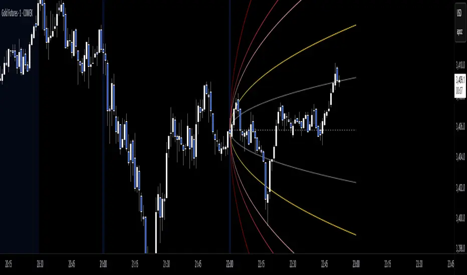
StatPivot- Dynamic Range Analyzer - indicator [PresentTrading]Hello everyone! In the following few open scripts, I would like to share various statistical tools that benefit trading. For this time, it is a powerful indicator called StatPivot- Dynamic Range Analyzer that brings a whole new dimension to your technical analysis toolkit.
This tool goes beyond traditional pivot point analysis by providing comprehensive statistical insights about price movements, helping you identify high-probability trading opportunities based on historical data patterns rather than subjective interpretations. Whether you're a day trader, swing trader, or position trader, StatPivot's real-time percentile rankings give you a statistical edge in understanding exactly where current price action stands within historical contexts.
Welcome to share your opinions! Looking forward to sharing the next tool soon!
█ Introduction and How it is Different
StatPivot is an advanced technical analysis tool that revolutionizes retracement analysis. Unlike traditional pivot indicators that only show static support/resistance levels, StatPivot delivers dynamic statistical insights based on historical pivot patterns.
Its key innovation is real-time percentile calculation - while conventional tools require new pivot formations before updating (often too late for trading decisions), StatPivot continuously analyzes where current price stands within historical retracement distributions.
Furthermore, StatPivot provides comprehensive statistical metrics including mean, median, standard deviation, and percentile distributions of price movements, giving traders a probabilistic edge by revealing which price levels represent statistically significant zones for potential reversals or continuations. By transforming raw price data into statistical insights, StatPivot helps traders move beyond subjective price analysis to evidence-based decision making.
█ Strategy, How it Works: Detailed Explanation
🔶 Pivot Point Detection and Analysis
The core of StatPivot's functionality begins with identifying significant pivot points in the price structure. Using the parameters left and right, the indicator locates pivot highs and lows by examining a specified number of bars to the left and right of each potential pivot point:
Copyp_low = ta.pivotlow(low, left, right)
p_high = ta.pivothigh(high, left, right)
For a point to qualify as a pivot low, it must have left higher lows to its left and right higher lows to its right. Similarly, a pivot high must have left lower highs to its left and right lower highs to its right. This approach ensures that only significant turning points are recognized.
🔶 Percentage Change Calculation
Once pivot points are identified, StatPivot calculates the percentage changes between consecutive pivot points:
For drops (when a pivot low is lower than the previous pivot low):
CopydropPercent = (previous_pivot_low - current_pivot_low) / previous_pivot_low * 100
For rises (when a pivot high is higher than the previous pivot high):
CopyrisePercent = (current_pivot_high - previous_pivot_high) / previous_pivot_high * 100
These calculations quantify the magnitude of each market swing, allowing for statistical analysis of historical price movements.
🔶 Statistical Distribution Analysis
StatPivot computes comprehensive statistics on the historical distribution of drops and rises:
Average (Mean): The arithmetic mean of all recorded percentage changes
CopyavgDrop = array.avg(dropValues)
Median: The middle value when all percentage changes are arranged in order
CopymedianDrop = array.median(dropValues)
Standard Deviation: Measures the dispersion of percentage changes from the average
CopystdDevDrop = array.stdev(dropValues)
Percentiles (25th, 75th): Values below which 25% and 75% of observations fall
Copyq1 = array.get(sorted, math.floor(cnt * 0.25))
q3 = array.get(sorted, math.floor(cnt * 0.75))
VaR95: The maximum expected percentage drop with 95% confidence
Copyvar95D = array.get(sortedD, math.floor(nD * 0.95))
Coefficient of Variation (CV): Measures relative variability
CopycvD = stdDevDrop / avgDrop
These statistics provide a comprehensive view of market behavior, enabling traders to understand the typical ranges and extreme moves.
🔶 Real-time Percentile Ranking
StatPivot's most innovative feature is its real-time percentile calculation. For each current price, it calculates:
The percentage drop from the latest pivot high:
CopycurrentDropPct = (latestPivotHigh - close) / latestPivotHigh * 100
The percentage rise from the latest pivot low:
CopycurrentRisePct = (close - latestPivotLow) / latestPivotLow * 100
The percentile ranks of these values within the historical distribution:
CopyrealtimeDropRank = (count of historical drops <= currentDropPct) / total drops * 100
This calculation reveals exactly where the current price movement stands in relation to all historical movements, providing crucial context for decision-making.
🔶 Cluster Analysis
To identify the most common retracement zones, StatPivot performs a cluster analysis by dividing the range of historical drops into five equal intervals:
CopyrangeSize = maxVal - minVal
For each interval boundary:
Copyboundaries = minVal + rangeSize * i / 5
By counting the number of observations in each interval, the indicator identifies the most frequently occurring retracement zones, which often serve as significant support or resistance areas.
🔶 Expected Price Targets
Using the statistical data, StatPivot calculates expected price targets:
CopytargetBuyPrice = close * (1 - avgDrop / 100)
targetSellPrice = close * (1 + avgRise / 100)
These targets represent statistically probable price levels for potential entries and exits based on the average historical behavior of the market.
█ Trade Direction
StatPivot functions as an analytical tool rather than a direct trading signal generator, providing statistical insights that can be applied to various trading strategies. However, the data it generates can be interpreted for different trade directions:
For Long Trades:
Entry considerations: Look for price drops that reach the 70-80th percentile range in the historical distribution, suggesting a statistically significant retracement
Target setting: Use the Expected Sell price or consider the average rise percentage as a reasonable target
Risk management: Set stop losses below recent pivot lows or at a distance related to the statistical volatility (standard deviation)
For Short Trades:
Entry considerations: Look for price rises that reach the 70-80th percentile range, indicating an unusual extension
Target setting: Use the Expected Buy price or average drop percentage as a target
Risk management: Set stop losses above recent pivot highs or based on statistical measures of volatility
For Range Trading:
Use the most common drop and rise clusters to identify probable reversal zones
Trade bounces between these statistically significant levels
For Trend Following:
Confirm trend strength by analyzing consecutive higher pivot lows (uptrend) or lower pivot highs (downtrend)
Use lower percentile retracements (20-30th percentile) as entry opportunities in established trends
█ Usage
StatPivot offers multiple ways to integrate its statistical insights into your trading workflow:
Statistical Table Analysis: Review the comprehensive statistics displayed in the data table to understand the market's behavior. Pay particular attention to:
Average drop and rise percentages to set reasonable expectations
Standard deviation to gauge volatility
VaR95 for risk assessment
Real-time Percentile Monitoring: Watch the real-time percentile display to see where the current price movement stands within the historical distribution. This can help identify:
Extreme movements (90th+ percentile) that might indicate reversal opportunities
Typical retracements (40-60th percentile) that might continue further
Shallow pullbacks (10-30th percentile) that might represent continuation opportunities in trends
Support and Resistance Identification: Utilize the plotted pivot points as key support and resistance levels, especially when they align with statistically significant percentile ranges.
Target Price Setting: Use the expected buy and sell prices calculated from historical averages as initial targets for your trades.
Risk Management: Apply the statistical measurements like standard deviation and VaR95 to set appropriate stop loss levels that account for the market's historical volatility.
Pattern Recognition: Over time, learn to recognize when certain percentile levels consistently lead to reversals or continuations in your specific market, and develop personalized strategies based on these observations.
█ Default Settings
The default settings of StatPivot have been carefully calibrated to provide reliable statistical analysis across a variety of markets and timeframes, but understanding their effects allows for optimal customization:
Left Bars (30) and Right Bars (30): These parameters determine how pivot points are identified. With both set to 30 by default:
A pivot low must be the lowest point among 30 bars to its left and 30 bars to its right
A pivot high must be the highest point among 30 bars to its left and 30 bars to its right
Effect on performance: Larger values create fewer but more significant pivot points, reducing noise but potentially missing important market structures. Smaller values generate more pivot points, capturing more nuanced movements but potentially including noise.
Table Position (Top Right): Determines where the statistical data table appears on the chart.
Effect on performance: No impact on analytical performance, purely a visual preference.
Show Distribution Histogram (False): Controls whether the distribution histogram of drop percentages is displayed.
Effect on performance: Enabling this provides visual insight into the distribution of retracements but can clutter the chart.
Show Real-time Percentile (True): Toggles the display of real-time percentile rankings.
Effect on performance: A critical setting that enables the dynamic analysis of current price movements. Disabling this removes one of the key advantages of the indicator.
Real-time Percentile Display Mode (Label): Chooses between label display or indicator line for percentile rankings.
Effect on performance: Labels provide precise information at the current price point, while indicator lines show the evolution of percentile rankings over time.
Advanced Considerations for Settings Optimization:
Timeframe Adjustment: Higher timeframes generally benefit from larger Left/Right values to identify truly significant pivots, while lower timeframes may require smaller values to capture shorter-term swings.
Volatility-Based Tuning: In highly volatile markets, consider increasing the Left/Right values to filter out noise. In less volatile conditions, lower values can help identify more potential entry and exit points.
Market-Specific Optimization: Different markets (forex, stocks, commodities) display different retracement patterns. Monitor the statistics table to see if your market typically shows larger or smaller retracements than the current settings are optimized for.
Trading Style Alignment: Adjust the settings to match your trading timeframe. Day traders might prefer settings that identify shorter-term pivots (smaller Left/Right values), while swing traders benefit from more significant pivots (larger Left/Right values).
By understanding how these settings affect the analysis and customizing them to your specific market and trading style, you can maximize the effectiveness of StatPivot as a powerful statistical tool for identifying high-probability trading opportunities.
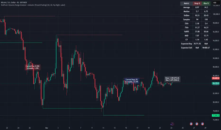
DCA Simulation for CryptoCommunity v1.1Overview
This script provides a detailed simulation of a Dollar-Cost Averaging (DCA) strategy tailored for crypto traders. It allows users to visualize how their DCA strategy would perform historically under specific parameters. The script is designed to help traders understand the mechanics of DCA and how it influences average price movement, budget utilization, and trade outcomes.
Key Features:
Combines Interval and Safety Order DCA:
Interval DCA: Regular purchases based on predefined time intervals.
Safety Order DCA: Additional buys triggered by percentage price drops.
Interactive Visualization:
Displays buy levels, average price, and profit-taking points on the chart.
Allows traders to assess how their strategy adapts to price movements.
Comprehensive Dashboard:
Tracks money spent, contracts acquired, and budget utilization.
Shows maximum amounts used if profit-taking is active.
Dynamic Safety Orders:
Resets safety orders when a new higher high is established.
Customizable Parameters:
Adjustable buy frequency, safety order settings, and profit-taking levels.
Suitable for traders with varying budgets and risk tolerances.
Default Strategy Settings:
Account Size: Default account size is set to $10,000 to represent a realistic budget for the average trader.
Commission & Slippage: Includes realistic trading fees and slippage assumptions to ensure accurate backtesting results.
Risk Management: Defaults to risking no more than 5% of the account balance per trade.
Sample Size: Optimized to generate a minimum of 100 trades for meaningful statistical analysis. Users can adjust parameters to fit longer timeframes or different datasets.
Usage Instructions:
Configure Your Strategy: Set the base order, safety order size, and buy frequency based on your preferred DCA approach.
Analyze Historical Performance: Use the chart and dashboard to understand how the strategy performs under different market conditions.
Optimize Parameters: Adjust settings to align with your risk tolerance and trading objectives.
Important Notes:
This script is for educational and simulation purposes. It is not intended to provide financial advice or guarantee profitability.
If the strategy's default settings do not meet your needs, feel free to adjust them while keeping risk management in mind.
TradingView limits the number of open trades to 999, so reduce the buy frequency if necessary to fit longer timeframes.
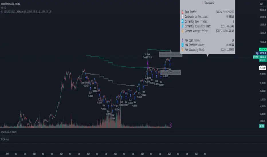
Quantile Statistical Levels [keypoems]Overview:
The Quantile Statistical Levels Indicator is designed to enhance intra-day trading strategies by leveraging statistical analysis of historical price movements.
The indicator is based on the principle that HTF (higher time-frame ) candles typically follow a pattern of:
1. Accumulation
2. Manipulation (can be modelled as the wick of the candle)
3. Expansion (the main price move)
A well-known trading technique involves buying within the wick of a bullish HTF candle, below its opening price, expecting an expansion of the current HTF candle (reverse for bearish). This indicator surfaces weeks of work on statistical distributions measuring the average length of the "manipulation" wicks of HTF candles, based on extensive historical data across multiple assets.
Features:
Statistical Quantile Manipulation and Expansion Levels:
This indicator marks Quantile Manipulation (and respective Expansion) levels that can help a trader gauge the shape of the currently developing HTF candle while looking at a a lower timeframe chart.
Q1 (First Quartile): statistically is a level touched 3 out of 4 times (75% of the time).
Median (Q2): it is a price threshold touched 50% of the time.
Q3 (Third Quartile): it is surpassed only 1 in 4 times (25% of the time), indicating significant price movement beyond this level is generally less common.
Warning Bands
The indicator also provides Warning Bands, these bands visually alert traders when the current price action is in a "Manipulation Zone" contrary to their intended trading bias. For instance, if a trader is looking to go long but the price is in the Manipulation Zone for shorts, this could signal a potential trap or a need for caution.
More precise levels can be optionally activated in the options for specific markets (currently NQ).

MathHelpersLibrary "MathHelpers"
Overview
A collection of helper functions for designing indicators and strategies.
calculateATR(length, log)
Calculates the Average True Range (ATR) or Log ATR based on the 'log' parameter. Sans Wilder's Smoothing
Parameters:
length (simple int)
log (simple bool)
Returns: float The calculated ATR value. Returns Log ATR if `log` is true, otherwise returns standard ATR.
CDF(z)
Computes the Cumulative Distribution Function (CDF) for a given value 'z', mimicking the CDF function in "Statistically Sound Indicators" by Timothy Masters.
Parameters:
z (simple float)
Returns: float The CDF value corresponding to the input `z`, ranging between 0 and 1.
logReturns(lookback)
Calculates the logarithmic returns over a specified lookback period.
Parameters:
lookback (simple int)
Returns: float The calculated logarithmic return. Returns `na` if insufficient data is available.