STD-Filtered, Gaussian-Kernel-Weighted Moving Average [Loxx]STD-Filtered, Gaussian-Kernel-Weighted Moving Average is a moving average that weights price by using a Gaussian kernel function to calculate data points. This indicator also allows for filtering both source input price and output signal using a standard deviation filter.
Purpose
This purpose of this indicator is to take the concept of Kernel estimation and apply it in a way where instead of predicting past values, the weighted function predicts the current bar value at each bar to create a moving average that is suitable for trading. Normally this method is used to create an array of past estimators to model past data but this method is not useful for trading as the past values will repaint. This moving average does NOT repaint, however you much allow signals to close on the current bar before taking the signal. You can compare this to Nadaraya-Watson Estimator wherein they use Nadaraya-Watson estimator method with normalized kernel weighted function to model price.
What are Kernel Functions?
A kernel function is used as a weighing function to develop non-parametric regression model is discussed. In the beginning of the article, a brief discussion about properties of kernel functions and steps to build kernels around data points are presented.
Kernel Function
In non-parametric statistics, a kernel is a weighting function which satisfies the following properties.
A kernel function must be symmetrical. Mathematically this property can be expressed as K (-u) = K (+u). The symmetric property of kernel function enables its maximum value (max(K(u)) to lie in the middle of the curve.
The area under the curve of the function must be equal to one. Mathematically, this property is expressed as: integral −∞ + ∞ ∫ K(u)d(u) = 1
Value of kernel function can not be negative i.e. K(u) ≥ 0 for all −∞ < u < ∞.
Kernel Estimation
In this article, Gaussian kernel function is used to calculate kernels for the data points. The equation for Gaussian kernel is:
K(u) = (1 / sqrt(2pi)) * e^(-0.5 *(j / bw)^2)
Where xi is the observed data point. j is the value where kernel function is computed and bw is called the bandwidth. Bandwidth in kernel regression is called the smoothing parameter because it controls variance and bias in the output. The effect of bandwidth value on model prediction is discussed later in this article.
Included
Loxx's Expanded Source types
Signals
Alerts
Bar coloring
Kernel
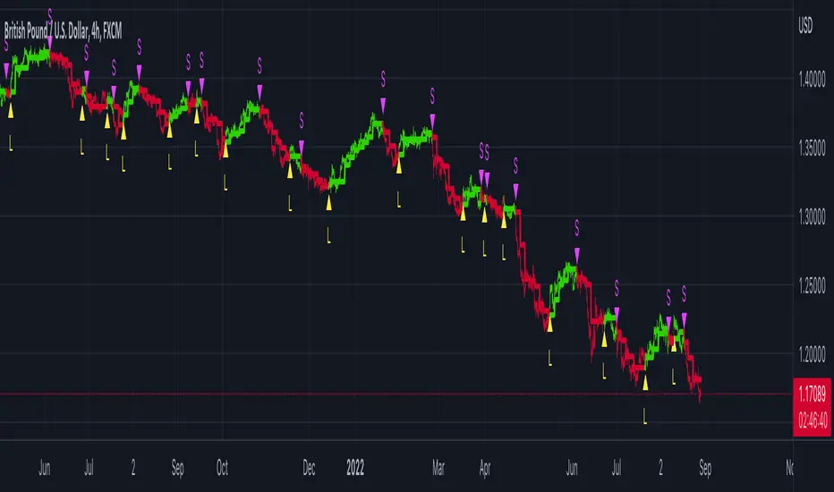
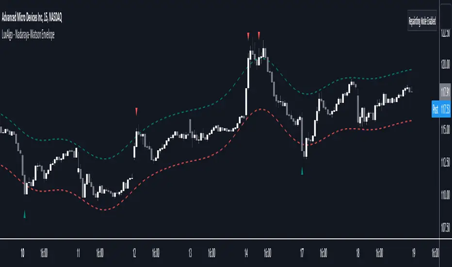
Nadaraya-Watson Envelope [LuxAlgo]This indicator builds upon the previously posted Nadaraya-Watson smoothers. Here we have created an envelope indicator based on Kernel Smoothing with integrated alerts from crosses between the price and envelope extremities. Unlike the Nadaraya-Watson estimator, this indicator follows a contrarian methodology.
Please note that by default this indicator can be subject to repainting. Users can use a non-repainting smoothing method available from the settings. The triangle labels are designed so that the indicator remains useful in real-time applications.
🔶 USAGE
🔹 Non Repainting
This tool can outline extremes made by the prices. This is achieved by estimating the underlying trend in the price, then calculating the mean absolute deviations from it, the obtained result is added/subtracted to the estimated underlying trend.
The non-repainting method estimates the underlying trend in price using an "endpoint Nadaraya-Watson estimator", and would return similar results to more classical band indicators.
🔹 Repainting
The repainting method makes use of the Nadaraya-Watson estimator to estimate the underlying trend in the price. The construction of the band extremities is the same as in the non-repainting method.
We can expect the price to reverse when crossing one of the envelope extremities. Crosses between the price and the envelopes extremities are indicated with triangles on the chart.
For real-time applications, triangles are always displayed when a cross occurs and remain displayed at the location it first appeared even if the cross is no longer visible after a recalculation of the envelope.
By popular demand, we have integrated alerts for this indicator from the crosses between the price and the envelope extremities. However, we do not recommend this precise method to be used alone or for solely real-time applications. We do not have data supporting the performance of this tool over more classical bands/envelope/channels indicators.
🔶 SETTINGS
Bandwidth: Controls the degree of smoothness of the envelopes, with higher values returning smoother results.
Mult: Controls the envelope width.
Source: Input source of the indicator.
Repainting Smoothing: Determine if a repainting or non-repainting method should be used for the calculation of the indicator.
🔶 RELATED SCRIPTS
For more information on the Nadaraya-Watson estimator see:
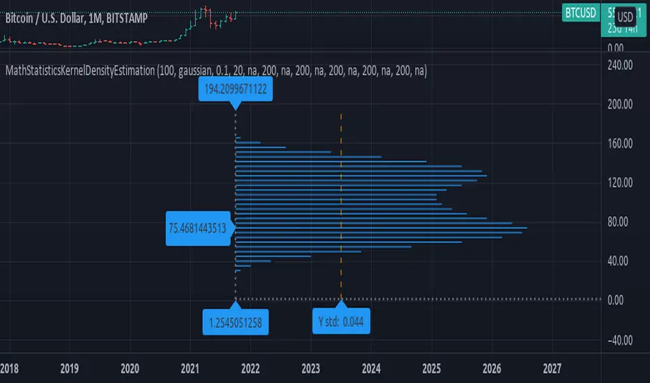
MathStatisticsKernelDensityEstimationLibrary "MathStatisticsKernelDensityEstimation"
(KDE) Method for Kernel Density Estimation
kde(observations, kernel, bandwidth, nsteps)
Parameters:
observations : float array, sample data.
kernel : string, the kernel to use, default='gaussian', options='uniform', 'triangle', 'epanechnikov', 'quartic', 'triweight', 'gaussian', 'cosine', 'logistic', 'sigmoid'.
bandwidth : float, bandwidth to use in kernel, default=0.5, range=(0, +inf), less will smooth the data.
nsteps : int, number of steps in range of distribution, default=20, this value is connected to how many line objects you can display per script.
Returns: tuple with signature: (float array, float array)
draw_horizontal(distribution_x, distribution_y, distribution_lines, graph_lines, graph_labels) Draw a horizontal distribution at current location on chart.
Parameters:
distribution_x : float array, distribution points x value.
distribution_y : float array, distribution points y value.
distribution_lines : line array, array to append the distribution curve lines.
graph_lines : line array, array to append the graph lines.
graph_labels : label array, array to append the graph labels.
Returns: void, updates arrays: distribution_lines, graph_lines, graph_labels.
draw_vertical(distribution_x, distribution_y, distribution_lines, graph_lines, graph_labels) Draw a vertical distribution at current location on chart.
Parameters:
distribution_x : float array, distribution points x value.
distribution_y : float array, distribution points y value.
distribution_lines : line array, array to append the distribution curve lines.
graph_lines : line array, array to append the graph lines.
graph_labels : label array, array to append the graph labels.
Returns: void, updates arrays: distribution_lines, graph_lines, graph_labels.
style_distribution(lines, horizontal, to_histogram, line_color, line_style, linewidth) Style the distribution lines.
Parameters:
lines : line array, distribution lines to style.
horizontal : bool, default=true, if the display is horizontal(true) or vertical(false).
to_histogram : bool, default=false, if graph style should be switched to histogram.
line_color : color, default=na, if defined will change the color of the lines.
line_style : string, defaul=na, if defined will change the line style, options=('na', line.style_solid, line.style_dotted, line.style_dashed, line.style_arrow_right, line.style_arrow_left, line.style_arrow_both)
linewidth : int, default=na, if defined will change the line width.
Returns: void.
style_graph(lines, lines, horizontal, line_color, line_style, linewidth) Style the graph lines and labels
Parameters:
lines : line array, graph lines to style.
lines : labels array, graph labels to style.
horizontal : bool, default=true, if the display is horizontal(true) or vertical(false).
line_color : color, default=na, if defined will change the color of the lines.
line_style : string, defaul=na, if defined will change the line style, options=('na', line.style_solid, line.style_dotted, line.style_dashed, line.style_arrow_right, line.style_arrow_left, line.style_arrow_both)
linewidth : int, default=na, if defined will change the line width.
Returns: void.
Nadaraya-Watson Smoothers [LuxAlgo]The following tool smoothes the price data using various methods derived from the Nadaraya-Watson estimator, a simple Kernel regression method. This method makes use of the Gaussian kernel as a weighting function.
Users have the option to use a non-repainting as well as a repainting method, see the USAGE section for more information.
🔶 USAGE
🔹 Non Repainting
When Repainting Smoothing is disabled the returned indicator acts similarly to a regular causal moving average. This result could be described as an "endpoint Nadaraya-Watson estimator".
Unlike a regular moving average whose degree of smoothness is commonly determined by the length of its calculation window, the degree of smoothness of the proposed indicator is determined by the bandwidth setting, with a higher value returning smoother results.
In the above chart, a bandwidth value of 50 is used. An increasing value of the smoother is indicative of an uptrend, while a decreasing value is indicative of a downtrend.
🔹 Repainting
Non-causal smoothing methods have found low support from technical analysts because they tend to repaint. Yet, they can provide powerful insights such as estimating underlying trends in the price as well as seeing how far prices deviate from them. They can also make drawing certain patterns easier and can help see underlying structures in the price more clearly.
Using higher bandwidth values allows for estimating longer-term trends in the price.
Triangular labels highlight points where the direction of the estimator change. This allows for the identification of tops and bottoms in the underlying trend which can be compared to the actual price tops and bottoms.
Note that multiple labels can appear in real time, highlighting real-time changes in the estimator's direction. The most recent label on a series of labels is the first to appear. This can eventually be useful for the real-time predictive application of the estimator. However, it is not a usage we particularly recommend.
🔶 DETAILS
The Nadaraya-Watson estimator can be described as a series of weighted averages using a specific normalized kernel as a weighting function. For each point of the estimator at time t , the peak of the kernel is located at time t , as such the highest weights are attributed to values neighboring the price located at time t .
A lower bandwidth value would contribute toward a more important weighting of the price at a precise point and would as such less smooth results. In the case where our bandwidth is so small that the resulting kernel is just an impulse, we would get the raw price back.
However, when the bandwidth is sufficiently large, prices would be weighted similarly, thus resulting in a result closer to the price mean.
It can be interesting to note that due to the nature of the estimator and its weighting procedure, real-time results would not deviate drastically for points in the estimator near the center of the calculation window.
🔶 SETTINGS
Bandwidth : controls the bandwidth of the Gaussian kernel, with higher values returning smoother results.
Src : Input source of the kernel regression.
Repainting Smoothing : Determine if the smoothing method should repaint or not. If disabled the "endpoint Nadaraya-Watson estimator" is returned.

Adjustable MA & Alternating Extremities [LuxAlgo]Returns a moving average allowing the user to control the amount of lag as well as the amplitude of its overshoots thanks to a parametric kernel. The indicator displays alternating extremities and aims to provide potential points where price might reverse.
Due to user requests, we added the option to display the moving average as candles instead of a solid line.
Settings
Length: MA period, refers to the number of most recent data points to use for its calculation.
Mult: Multiplicative factor for each extremity.
As Smoothed Candles: Allows the user to show the MA as a series of candles instead of a solid line.
Show Alternating Extremities : Determines whether to display the alternating extremities or not.
Lag: Controls the amount of lag of the MA, with higher values returning a MA with more lag.
Overshoot: Controls the amplitude of the overshoots returned by the MA, with higher values increasing the amplitude of the overshoots.
Usage
Moving averages using parametric kernels allows users to have more control over characteristics such as lag or smoothness; this can greatly benefit the analyst. A moving average with reduced lag can be used as a leading moving average in a MA crossover system, while lag will benefit moving averages used as slow MA in a crossover system.
Increasing 'Lag' will increase smoothness while increasing 'overshoot' will reduce lag.
The following indicator puts more emphasis on its alternating extremities, an upper extremity will be shown once the high price crosses the upper extremity, while a low extremity will be shown once the low price crosses the lower extremity. These can be interpreted like extremities of a band indicator.
The MA using a length value of 200 with a multiplicative factor of 1.
In general, extremities will effectively return points where price might potentially bounce in ranging markets while closing prices under trending markets will often be found above an upper extremity and under a lower extremity.
Reducing the lag of the moving average allows the user to obtain a more timely estimate of the underlying trend in the price, with a better fit overall. This allows the user to obtain potentially pertinent extremities where price might reverse upon a break, even under trending markets.
In the above chart, the price initially breaks the upper extremity, however, we can observe that the upper extremity eventually reaches back the price, goes above it, provides a resistance, and effectively indicates a reversal.
Users can plot candles from the moving average, these are fairly similar to heikin-ashi candles in the sense that CandleOpen(t) ≠ CandleClose(t-1) , each point of the candle is calculated as follows for our indicator:
Open = Average between MA(t-1) and MA(t-2)
High = MA using the high price as input
Low = MA using the low price as input
Close = MA using the closing price as input
Details
Lag is defined as the effect of moving averages to reflect past price variations instead of new ones, lag can be observed by the user and is the main cause of false signals. Lag is proportional to the degree of filtering returned by the moving average.
Overshooting is a common effect encountered in non-lagging moving averages, and is defined as the tendency of a moving average to exceed a maximum level (or minimum level, which can be defined as undershooting )
MA and rolling maximum/minimum, both using a length of 50 bars. While we can think of lag as a cost of smoothness, we can think of overshooting as a cost for reduced lag on some occasions.
Explaining the kernel design behind our moving average requires understanding of the logic behind lag reduction in moving averages. This can prove to be complex for non informed users, but let's just focus on the simpler part; moving averages can be defined as a weighted sum between past prices and a set of coefficients (kernel).
MA(t) = b(0)C(t) + b(1)C(t-1) + b(2)C(t-2) + ... + b(n-1)C(t-n-1)
Where n is the period of the moving average. Lag is (non optimally) reduced by "underweighting" past prices - that is multiplying them by negative numbers.
The kernel used in our moving average is based on a modified sinewave. A weighted sum making use of a sinewave as a kernel would return an oscillator centered at 0. We can divide this sinewave by an increasing linear function in order to obtain a kernel allowing us to obtain a low lag moving average instead of a centered oscillator. This is the main idea in the design of the kernel used by our moving average.
The kernel equation of our moving average is:
sin(2πx^α)(1 - x^β)
With 1>x>0 , and where α controls the lag, while β controls the overshoot amplitude.
Using this equation we can obtain the following kernels:
Here only α is changed, while β is equal to 1. Values to the left would represent the coefficients for the most recent prices. Notice how the most significant coefficients are given to the oldest prices in the case where α increases.
Higher overshoot would require more negative values, this is controlled by β
Here only β is changed, while α is equal to 1. Notice how higher values return lower negative coefficients. This effectively increases the overshoots amplitude in our moving average. We can decrease α in order for these negative coefficients to underweight more recent values.
Using α = 0 allows us to simplify the kernel equation to:
1 - x^β
Using this kernel we can obtain more classical moving averages, this can be seen from the following results:
Using β = 1 allows us to obtain a linearly decreasing kernel (the one of a WMA), while increasing allows the kernel to converge toward a rectangular kernel (the one of SMA).

Function - Kernel Density Estimation (KDE)"In statistics, kernel density estimation (KDE) is a non-parametric way to estimate the probability density function of a random variable."
from wikipedia.com
KDE function with optional kernel:
Uniform
Triangle
Epanechnikov
Quartic
Triweight
Gaussian
Cosinus
Republishing due to change of function.
deprecated script:

KDE-Gaussian"In statistics, kernel density estimation (KDE) is a non-parametric way to estimate the probability density function of a random variable."
from wikipedia.com

Blackman Filter - The Smoother The BetterIntroduction
Who doesn't like smooth things? I'd like a smooth market price for christmas! But i can't get it, instead its so noisy...so you apply a filter to smooth it, such filters are called low-pass filters, they smooth and its great but they have lag, so nobody really use them, but they are pretty to look at.
Its on a childish note that i will introduce this indicator, so what it is all about? I propose a new FIR filter using a blackman function as filter kernel for financial time-series smoothing, do you prefer the childish tone ? Fear not its surprisingly easy!
The Blackman Function
The blackman function look like a bell shaped curve, look:
The blackman function will produce such curve. This function is called a cosine sum function because she is based on the sum of cosine functions, here only 2.
0.42 - 0.5 * cos(2 * pi * k) + 0.08 * cos(4 * pi * k)
Originally you use this function for windowing , what does it means? In signal processing you have a function called sync function , if you use this function as filter kernel you would get the ideal frequency domain response filter, sometime called brickwall filter, it would be extremely smooth.
Above the optimal low pass filter frequency response.
However the sync function has no ending values and goes on forever, therefore we can't use it for convolution, expect if we apply windowing. Filters using windowing are called windowed-sinc filters, i will describe the procedure below :
1 - Create a sync function = sin(pi*n)/(pi*n)
2 - Truncate it = I only keep the first length points of the sync function.
This create a abrupt end, the frequency of a filter using step 1 as kernel would contain ripples in the pass band and stop band, this is bad! The frequency response would look like this :
3 - I multiply my values of step 2 by a window function, it can the blackman window, i no longer have an abrupt end, its smooth!
The frequency response of the filter using this kernel would no longer have ripples! This is the power of windowing functions.
Here we are not using such thing, but we could in the future. Here instead we use the blackman function as filter kernel, because this function is bell shaped this mean that the filter will certainly be smooth (symmetrical weighting is a rule of thumb for kernels when we want really smooth filters).
The Filter
This filter is quite smooth, unlike the gaussian filter this filter give less weights to recent and past values, this is because the blackman function has fatter tails than the gaussian one. I could make a comparison of both, however they are quite alike, if you often use a gaussian filter its up to you to decide which one you prefer.
The filter can do a better job than the moving average when it comes to preserve the frequency components that constitute the cycles/trend.
We can see that the filter has a greater performance when it comes to keep the shape of the market price, thus it has a slightly better fit.
Conclusion
Ok so in this post you learned a bit about the sync function and windowing, those are basic subjects in signal processing, they allow us to approximate the filter with the ideal frequency response, i also showed you that those windowing function could be used as kernel and that they where pretty smooth on their own, there are many others, but the one i prefer is the blackman windowing function.
I know what you are thinking, "we want trailing stops, alerts, colors, arrows!", and i understand you pal, but sometimes its cool to take a break from all this stuff. However i can tell that i'am working on a side project that aim to estimate rolling maximum/minimum as fast as possible, any experiments will be published here, and i can ensure you that those indicators will make your day quite brighter, we will see that soon.
I hope you learned something from this post! I'am a bit tired (look i'am disappearing !)
Thanks for reading !

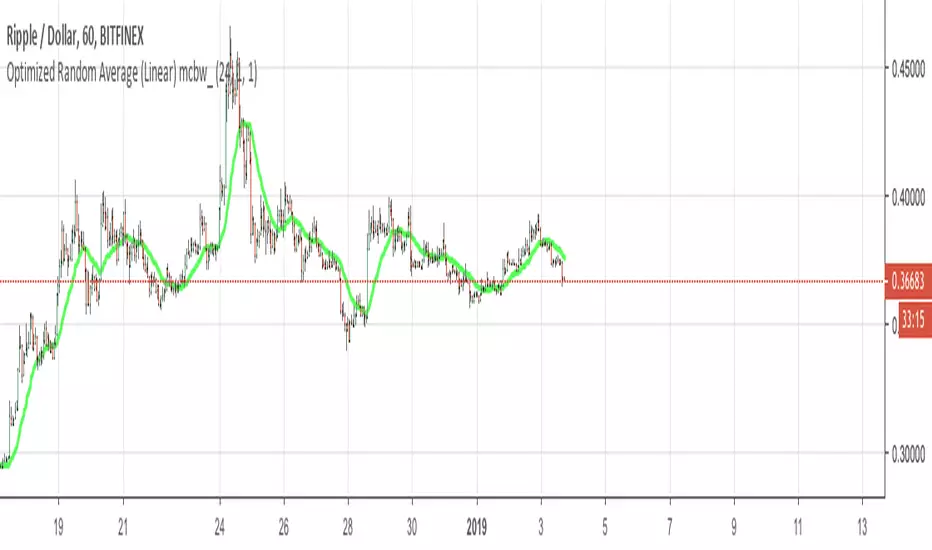
Optimized Random Average (Linear) mcbw_This is a moving average with a customizable random kernel. You can shape your kernel by selecting your parameters in the settings window. This is not something that is immediately ready to mess with by just applying it on the chart, it is very useful for people who are researching indicators and developing new tools. To see the shape of your kernel you can plug it into google or wolfram. This indicator and the related ones are rather technical in nature, so feel free to comment any questions you may have and to see if anyone has asked your question.
Read more here:
Happy studying and enjoy your life!
2019 will be absolutely insane!
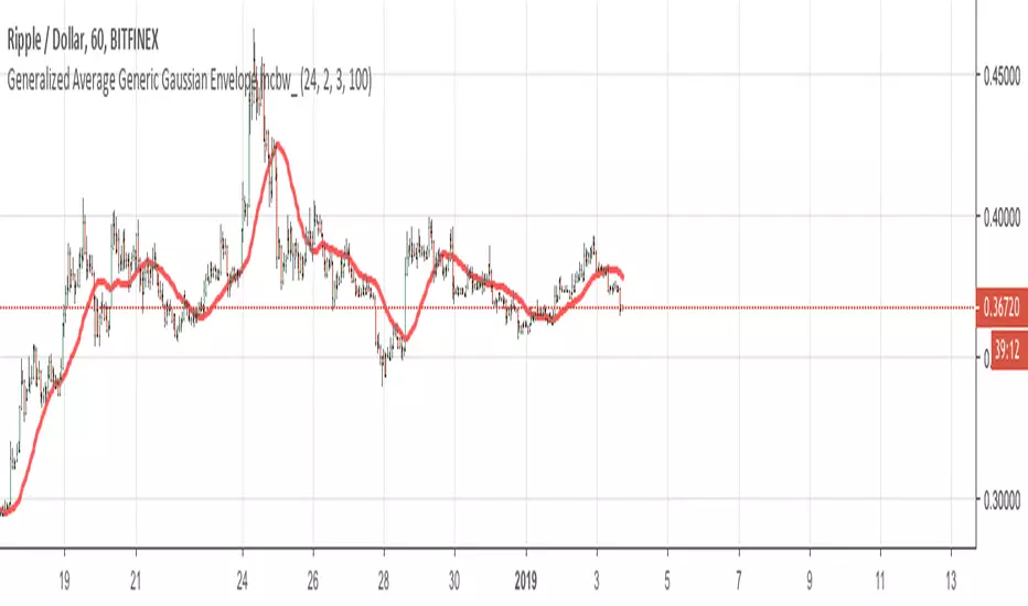
Generalized Average Generic Gaussian Envelope mcbw_This is a moving average with a customizable gaussian kernel. You can shape your kernel by selecting your parameters in the settings window. This is not something that is immediately ready to mess with by just applying it on the chart, it is very useful for people who are researching indicators and developing new tools. To see the shape of your kernel you can plug it into google or wolfram. This indicator and the related ones are rather technical in nature, so feel free to comment any questions you may have and to see if anyone has asked your question.
Read more here:
Happy studying and enjoy your life!
2019 will be absolutely insane!
Generalized Average Polynomial Envelope mcbw_This is a moving average with a customizable polynomial kernel. You can shape your kernel by selecting your parameters in the settings window. This is not something that is immediately ready to mess with by just applying it on the chart, it is very useful for people who are researching indicators and developing new tools. To see the shape of your kernel you can plug it into google or wolfram. This indicator and the related ones are rather technical in nature, so feel free to comment any questions you may have and to see if anyone has asked your question.
Read more here:
Happy studying and enjoy your life!
2019 will be absolutely insane!
