EWMA Implied Volatility based on Historical VolatilityVolatility is the most common measure of risk.
Volatility in this sense can either be historical volatility (one observed from past data), or it could implied volatility (observed from market prices of financial instruments.)
The main objective of EWMA is to estimate the next-day (or period) volatility of a time series and closely track the volatility as it changes.
The EWMA model allows one to calculate a value for a given time on the basis of the previous day's value.
The EWMA model has an advantage in comparison with SMA, because the EWMA has a memory.
The EWMA remembers a fraction of its past by a factor A, that makes the EWMA a good indicator of the history of the price movement if a wise choice of the term is made.
Full details regarding the formula :
www.investopedia.com
In this scenario, we are looking at the historical volatility using the anual length of 252 trading days and a monthly length of 21.
Once we apply all of that we are going to get the yearly volatility.
After that we just have to divide that by the square root of number of days in a year, or weeks in a year or months in a year in order to get the daily/weekly/monthly expected volatility.
Once we have the expected volatility, we can estimate with a high chance where the market top and bottom is going to be and continue our analysis on that premise.
If you have any questions, please let me know !
"implied"に関するスクリプトを検索

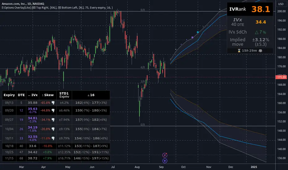
Options Overlay [Lite] IVR IV Skew Delta Expmv MurreyMath Expiry𝗡𝗼𝗻-𝗼𝗳𝗳𝗶𝗰𝗶𝗮𝗹 𝗧𝗢𝗦 𝗮𝗻𝗱 𝗧𝗮𝘀𝘁𝘆𝗧𝗿𝗮𝗱𝗲 𝗹𝗶𝗸𝗲 𝗜𝗩𝗥 𝗢𝗽𝘁𝗶𝗼𝗻𝘀 𝘃𝗶𝘀𝘂𝗮𝗹𝗶𝘇𝗮𝘁𝗶𝗼𝗻 𝘁𝗼𝗼𝗹 𝘄𝗶𝘁𝗵 𝗱𝗲𝗹𝗮𝘆𝗲𝗱 𝗼𝗽𝘁𝗶𝗼𝗻 𝗰𝗵𝗮𝗶𝗻 𝗱𝗮𝘁𝗮
Are you an options trader who uses TradingView for technical analysis for the US market?
➡️ Do you want to see the IV Rank of an instrument on TradingView?
➡️ Can’t you check the key options metrics while charting?
➡️ Have you never visualized the options chain before?
➡️ Would you like to see how the IVx has changed for a specific ticker?
If you answered "yes" to any of these questions, then we have the solution for you!
🔃 Auto-Updating Option Metrics without refresh!
🍒 Developed and maintained by option traders for option traders.
📈 Specifically designed for TradingView users who trade options.
Our indicator provides essential key metrics such as:
✅ IVRank
✅ IVx
✅ 5-Day IVx Change
✅ Delta curves and interpolated distances
✅ Expected move curve
✅ Standard deviation (STD1) curve
✅ Vertical Pricing Skew
✅ Horizontal IVx Skew
✅ Delta Skew
like TastyTrade, TOS, IBKR etc, but in a much more visually intuitive way. See detailed descriptions below.
If this isn't enough, we also include a unique grid system designed specifically for options traders. This package features our innovative dynamic grid system:
✅ Enhanced Murrey Math levels (horizontal scale)
✅ Options expirations (vertical scale)
Designed to help you assess market conditions and make well-informed trading decisions, this tool is an essential addition for every serious options trader!
Ticker Information:
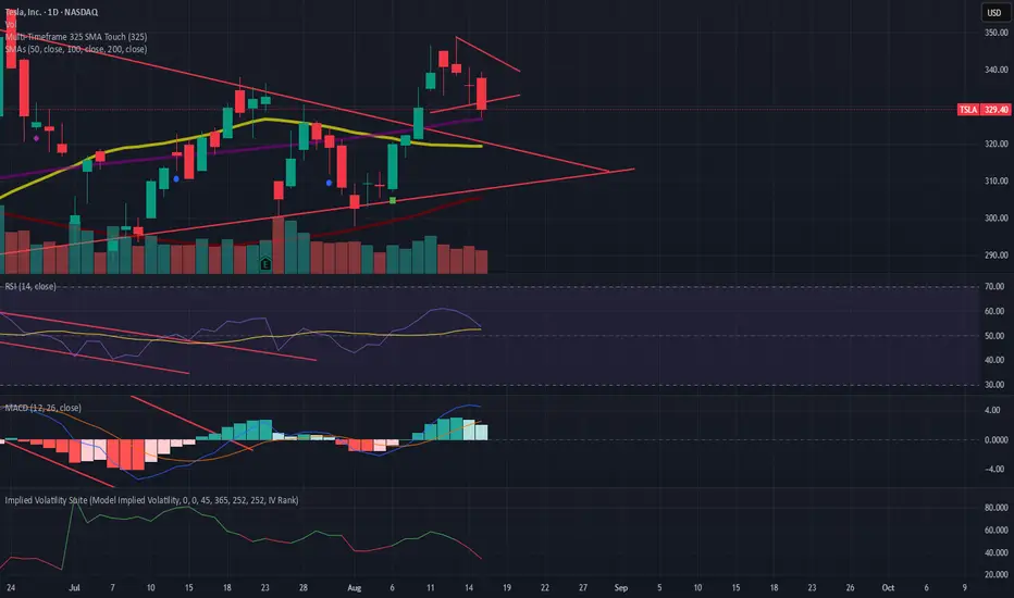
This indicator is currently implemented for 5 liquid tickers: NASDAQ:AAPL NASDAQ:AMZN AMEX:DIA NYSE:ORCL and NASDAQ:TSLA
How does the indicator work and why is it unique?
This Pine Script indicator is a complex tool designed to provide various option metrics and visualization tools for options market traders. The indicator extracts raw options data from an external data provider (ORATS), processes and refines the delayed data package using pineseed, and sends it to TradingView, visualizing the data using specific formulas (see detailed below) or interpolated values (e.g., delta distances). This method of incorporating options data into a visualization framework is unique and entirely innovative on TradingView.
The indicator aims to offer a comprehensive view of the current state of options for the implemented instruments, including implied volatility (IV), IV rank (IVR), options skew, and expected market movements, which are objectively measured as detailed below.
The options metrics we display may be familiar to options traders from various major brokerage platforms such as TastyTrade, IBKR, TOS, Tradier, TD Ameritrade, Schwab, etc.
Key Features:
IV Rank (IVR) : The implied volatility rank compares the current IV to the lowest and highest values over the past 52 weeks. The IVR indicator helps determine whether options are relatively cheap or expensive.
IV Average (IVx) : The implied volatility displayed in the options chain, calculated similarly to the VIX. IVx values are aggregated within the 35-70 day expiration cycle.
IV Change (5 days) : The change in implied volatility over the past five trading days. This indicator provides a quick insight into the recent changes in IV.
Expected Move (Exp. Move) : The expected movement for the options expiration cycle, calculated using the price of the ATM (at-the-money) straddle, the first OTM (out-of-the-money) strangle, and the second OTM strangle.
Options Skew : The price difference between put and call options with the same expiration date. Vertical and horizontal skew indicators help understand market sentiment and potential price movements.
Visualization Tools:
Informational IVR Panel : A tabular display mode that presents the selected indicators on the chart. The panel’s placement, size, and content are customizable, including color and tooltip settings.
1 STD, Delta, and Expected Move : Visualization of fundamental classic options metrics corresponding to expirations with bell curves.
Colored Label Tooltips : Detailed tooltips above the bell curves showing options metrics for each expiration.
Adaptive Murrey Math Lines : A horizontal line system based on the principles of Murrey Math Lines, helping identify important price levels and market structures.
Expiration Lines : Displays both monthly and weekly options expirations. The indicator supports various color and style settings, as well as the regulation of the number of expirations displayed.
🟨 𝗗𝗘𝗧𝗔𝗜𝗟𝗘𝗗 𝗗𝗢𝗖𝗨𝗠𝗘𝗡𝗧𝗔𝗧𝗜𝗢𝗡 🟨
🔶 Auto-Updating Option Metrics and Curved Lines
🔹 Interpolated DELTA Curves (16,20,25,30,40)
In our indicator, the curve layer settings allow you to choose the delta value for displaying the delta curve: 16, 20, 25, 30, or even 40. The color of the curve can be customized, and you can also hide the delta curve by selecting the "-" option.
It's important to mention that we display interpolated deltas from the actual option chain of the underlying asset using the Black-Scholes model. This ensures that the 16 delta truly reflects the theoretical, but accurate, 16 delta distance. (For example, deltas shown by brokerages for individual strikes are rounded; a 0.16 delta might actually be 0.1625.)
🔹 Expected Move Curve (Exp.mv)
The expected move is the predicted dollar change in the underlying stock's price by a given option's expiration date, with 68% certainty. It is calculated using the expiration's pricing and implied volatility levels. We chose the TastyTrade method for calculating expected move, as we found it to be the most expressive.
Expected Move Calculation
Expected Move = (ATM straddle price x 0.6) + (1st OTM strangle price x 0.3) + (2nd OTM strangle price x 0.1)
For example , if stock XYZ is trading at 121 and the ATM straddle is 4.40, the 120/122 strangle is 3.46, and the 119/123 strangle is 2.66, the expected move is calculated as follows: 4.40 x 0.60 = 2.64; 3.46 x 0.30 = 1.04; 2.66 x 0.10 = 0.27; Expected move = 2.64 + 1.04 + 0.27 = ±3.9
In this example below, the TastyTrade platform indicates the expected move on the option chain with a brown color, and the exact value is displayed behind the ± symbol for each expiration. By default, we also use brown for this indication, but this can be changed or the curve display can be turned off.
🔹 Standard Deviation Curve (1 STD)
One standard deviation of a stock encompasses approximately 68.2% of outcomes in a distribution of occurrences based on current implied volatility.
We use the expected move formula to calculate the one standard deviation range of a stock. This calculation is based on the days-to-expiration (DTE) of our option contract, the stock price, and the implied volatility of a stock:
Calculation:
Standard Deviation = Closing Price * Implied Volatility * sqrt(Days to Expiration / 365)
According to options literature, there is a 68% probability that the underlying asset will fall within this one standard deviation range at expiration.
If the 1 STD and Exp.mv displays are both enabled, the indicator fills the area between them with a light gray color. This is because both represent probability distributions that appear as a "bell curve" when graphed, making it visually appealing.
Tip and Note:
The 1 STD line might appear jagged at times , which does not indicate a problem with the indicator. This is normal immediately after market open (e.g., during the first data refresh of the day) or if the expirations are illiquid (e.g., weekly expirations). The 1 STD value is calculated based on the aggregated IVx for the expirations, and the aggregated IVx value for weekly expirations updates less frequently due to lower trading volume. In such cases, we recommend enabling the "Only Monthly Expirations" option to smooth out the bell curve.
∑ Quant Observation:
The values of the expected move and the 1st standard deviation (1STD) will not match because they use different calculation methods, even though both are referred to as representing 68% of the underlying asset's movement in options literature. The expected move is based on direct market pricing of ATM options. The 1STD, on the other hand, uses the averaged implied volatility (IVX) for the given expiration to determine its value. Based on our experience, it is better to consider the area between the expected move and the 1STD as the true representation of the original 68% rule.
🔶 IVR Dashboard Panel Rows
🔹 IVR (IV Rank)
The Implied Volatility Rank (IVR) indicator helps options traders assess the current level of implied volatility (IV) in comparison to the past 52 weeks. IVR is a useful metric to determine whether options are relatively cheap or expensive. This can guide traders on whether to buy or sell options. We calculate IVrank, like TastyTrade does.
IVR Calculation:
IV Rank = (current IV - 52 week IV low) / (52 week IV high - 52 week IV low)
IVR Levels and Interpretations:
IVR 0-10 (Green): Very low implied volatility rank. Options might be "cheap," potentially a good time to buy options.
IVR 10-35 (White): Normal implied volatility rank. Options pricing is relatively standard.
IVR 35-50 (Orange): Almost high implied volatility rank.
IVR 50-75 (Red): Definitely high implied volatility rank. Options might be "expensive," potentially a good time to sell options for higher premiums.
IVR above 75 (Highlighted Red): Ultra high implied volatility rank. Indicates very high levels, suggesting a favorable time for selling options.
The panel refreshes automatically if the symbol is implemented. You can hide the panel or change the position and size.
🔹IVx (Implied Volatility Index)
The Implied Volatility Index (IVx) displayed in the option chain is calculated similarly to the VIX. The Cboe uses standard and weekly SPX options to measure the expected volatility of the S&P 500. A similar method is utilized to calculate IVx for each option expiration cycle.
For our purposes on the IVR Panel, we aggregate the IVx values specifically for the 35-70 day monthly expiration cycle . This aggregated value is then presented in the screener and info panel, providing a clear and concise measure of implied volatility over this period.
IVx Color coding:
IVx above 30 is displayed in orange.
IVx above 60 is displayed in red
IVx on curve:
The IVx values for each expiration can be viewed by hovering the mouse over the colored tooltip labels above the Curve.
IVx avg on IVR panel :
If the option is checked in the IVR panel settings, the IVR panel will display the average IVx values up to the optimal expiration.
Important Note:
The IVx value alone does not provide sufficient context. There are stocks that inherently exhibit high IVx values. Therefore, it is crucial to consider IVx in conjunction with the Implied Volatility Rank (IVR), which measures the IVx relative to its own historical values. This combined view helps in accurately assessing the significance of the IVx in relation to the specific stock's typical volatility behavior.
This indicator offers traders a comprehensive view of implied volatility, assisting them in making informed decisions by highlighting both the absolute and relative volatility measures.
🔹IVx 5 days change %
We are displaying the five-day change of the IV Index (IVx value). The IV Index 5-Day Change column provides quick insight into recent expansions or decreases in implied volatility over the last five trading days.
Traders who expect the value of options to decrease might view a decrease in IVX as a positive signal. Strategies such as Strangle and Ratio Spread can benefit from this decrease.
On the other hand, traders anticipating further increases in IVX will focus on the rising IVX values. Strategies like Calendar Spread or Diagonal Spread can take advantage of increasing implied volatility.
This indicator helps traders quickly assess changes in implied volatility, enabling them to make informed decisions based on their trading strategies and market expectations.
🔹 Vertical Pricing Skew
At TanukiTrade, Vertical Pricing Skew refers to the difference in pricing between put and call options with the same expiration date at the same distance (at expected move). We analyze this skew to understand market sentiment. This is the same formula used by TastyTrade for calculations.
We calculate the interpolated strike price based on the expected move , taking into account the neighboring option prices and their distances. This allows us to accurately determine whether the CALL or PUT options are more expensive.
PUT Skew (red): Put options are more expensive than call options, indicating the market expects a downward move (▽). If put options are more expensive by more than 20% at the same expected move distance, we color it lighter red.
CALL Skew (green): Call options are more expensive than put options, indicating the market expects an upward move (△). If call options are priced more than 30% higher at the examined expiration, we color it lighter green.
Vertical Skew on Curve:
The degree of vertical pricing skew for each expiration can be viewed by hovering over the points above the curve. Hover with mouse for more information.
Vertical Skew on IVR panel:
We focus on options with 35-70 days to expiration (DTE) for optimal analysis in case of vertical skew. Hover with mouse for more information.
This approach helps us gauge market expectations accurately, providing insights into potential price movements. Remember, we always evaluate the skew at the expected move using linear interpolation to determine the theoretical pricing of options.
🔹 Delta Skew 🌪️ (Twist)
We have a new metric that examines which monthly expiration indicates a "Delta Skew Twist" where the 16 delta deviates from the monthly STD. This is important because, under normal circumstances, the 16 delta is positioned between the expected move and the standard deviation (STD1) line (see Exp.mv & 1STD exact definitions above). However, if the interpolated 16 delta line exceeds the STD1 line either upwards or downwards, it represents a special case of vertical skew on the option chain.
Normal case : exp.move < delta16 < std1
Delta Skew Twist: exp.move < std1 < delta16
We indicate this with direction-specific colors (red/green) on the delta line. We also color the section of the delta curve affected by the delta skew in this case, even if you choose to display a lower delta, such as 30, instead of 16.
If "Colored Labels with Tooltips" is enabled, we also display a 🌪️ symbol in the tooltip for the expirations affected by Delta Skew.
If you have enabled the display of 'Vertical Pricing Skew' on the IVR Panel, a 🌪️ symbol will also appear next to the value of the vertical skew, and the tooltip will indicate from which expiration Delta Skew is observed.
🔹 Horizontal IVx Skew
In options pricing, it is typically expected that the implied volatility (IVx) increases for options with later expiration dates. This means that options further out in time are generally more expensive. At TanukiTrade, we refer to the phenomenon where this expectation is reversed—when the IVx decreases between two consecutive expirations—as Horizontal Skew or IVx Skew.
Horizontal IVx Skew occurs when: Front Expiry IVx < Back Expiry IVx
This scenario can create opportunities for traders who prefer diagonal or calendar strategies . Based on our experience, we categorize Horizontal Skew into two types:
Weekly Horizontal Skew:
When IVx skew is observed between two consecutive non-monthly expirations, the displayed value is the rounded-up percentage difference. On hover, the approximate location of this skew is also displayed. The precise location can be seen on this indicator.
Monthly Horizontal Skew:
When IVx skew is observed between two consecutive monthly expirations , the displayed value is the rounded-up percentage difference. On hover, the approximate location of this skew is also displayed. The precise location can be seen on our Overlay indicator.
The Monthly Vertical IVx skew is consistently more liquid than the weekly vertical IVx skew. Weekly Horizontal IVx Skew may not carry relevant information for symbols not included in the 'Weeklies & Volume Masters' preset in our Options Screener indicator.
If the options chain follows the normal IVx pattern, no skew value is displayed.
Color codes or tooltip labels above curve:
Gray - No horizontal skew;
Purple - Weekly horizontal skew;
BigBlue - Monthly horizontal skew
The display of monthly and weekly IVx skew can be toggled on or off on the IVR panel. However, if you want to disable the colored tooltips above the curve, this can only be done using the "Colored labels with tooltips" switch.
We indicate this range with colorful information bubbles above the upper STD line.
🔶 The Option Trader’s GRID System: Adaptive MurreyMath + Expiry Lines
At TanukiTrade, we utilize Enhanced MurreyMath and Expiry lines to create a dynamic grid system, unlike the basic built-in vertical grids in TradingView, which provide no insight into specific price levels or option expirations.
These grids are beneficial because they provide a structured layout, making important price levels visible on the chart. The grid automatically resizes as the underlying asset's volatility changes, helping traders identify expected movements for various option expirations.
The Option Trader’s GRID System part of this indicator can be used without limitations for all instruments . There are no type or other restrictions, and it automatically scales to fit every asset. Even if we haven't implemented the option metrics for a particular underlying asset, the GRID system will still function!
🔹 SETUP OF YOUR OPTIONS GRID SYSTEM
You can setup your new grid system in 3 easy steps!
STEP1: Hide default horizontal grid lines in TradingView
Right-click on an empty area of your chart, then select “Settings.” In the Chart settings -> Canvas -> Grid lines section, disable the display of horizontal lines to avoid distraction.
SETUP STEP2: Scaling fix
Right-click on the price scale on the right side, then select "Scale price chart only" to prevent the chart from scaling to the new horizontal lines!
STEP3: Enable Tanuki Options Grid
As a final step, make sure that both the vertical (MurreyMath) and horizontal (Expiry) lines are enabled in the Grid section of our indicator.
You are done, enjoy the new grid system!
🔹 HORIZONTAL: Enhanced MurreyMath Lines
Murrey Math lines are based on the principles observed by William Gann, renowned for his market symmetry forecasts. Gann's techniques, such as Gann Angles, have been adapted by Murrey to make them more accessible to ordinary investors. According to Murrey, markets often correct at specific price levels, and breakouts or returns to these levels can signal good entry points for trades.
At TanukiTrade, we enhance these price levels based on our experience , ensuring a clear display. We acknowledge that while MurreyMath lines aren't infallible predictions, they are useful for identifying likely price movements over a given period (e.g., one month) if the market trend aligns.
Our opinion: MurreyMath lines are not crystal balls (like no other tool). They should be used to identify that if we are trading in the right direction, the price is likely to reach the next unit step within a unit time (e.g. monthly expiration).
One unit step is the distance between Murrey Math lines, such as between the 0/8 and 1/8 lines. This interval helps identify different quadrants and is crucial for recognizing support and resistance levels.
Some option traders use Murrey Math lines to gauge the movement speed of an instrument over a unit time. A quadrant encompasses 4 unit steps.
Key levels, according to TanukiTrade, include:
Of course, the lines can be toggled on or off, and their default color can also be changed.
🔹 VERTICAL: Expiry Lines
The indicator can display monthly and weekly expirations as dashed lines, with customizable colors. Weekly expirations will always appear in a lighter shade compared to monthly expirations.
Monthly Expiry Lines:
You can turn off the lines indicating monthly expirations, or set the direction (past/future/both) and the number of lines to be drawn.
Weekly Expiry Lines:
You can display weekly expirations pointing to the future. You can also turn them off or specify how many weeks ahead the lines should be drawn.
Of course, the lines can be toggled on or off, and their default color can also be changed.
TIP: Hide default vertical grid lines in TradingView
Right-click on an empty area of your chart, then select “Settings.” In the Chart settings -> Canvas -> Grid lines section, disable the display of vertical lines to avoid distraction. Same, like steps above at MurreyMath lines.
🔶 ADDITIONAL IMPORTANT COMMENTS
- U.S. market only:
Since we only deal with liquid option chains: this option indicator only works for the USA options market and do not include future contracts; we have implemented each selected symbol individually.
- Why is there a slight difference between the displayed data and my live brokerage data? There are two reasons for this, and one is beyond our control.
- Brokerage Calculation Differences:
Every brokerage has slight differences in how they calculate metrics like IV and IVx. If you open three windows for TOS, TastyTrade, and IBKR side by side, you will notice that the values are minimally different. We had to choose a standard, so we use the formulas and mathematical models described by TastyTrade when analyzing the options chain and drawing conclusions.
- Option-data update frequency:
According to TradingView's regulations and guidelines, we can update external data a maximum of 5 times per day. We strive to use these updates in the most optimal way:
(1st update) 15 minutes after U.S. market open
(2nd, 3rd, 4th updates) 1.5–3 hours during U.S. market open hours
(5th update) 10 minutes before market close.
You don’t need to refresh your window, our last refreshed data-pack is always automatically applied to your indicator , and you can see the time elapsed since the last update at the bottom of your indicator.
- Skewed Curves:
The delta, expected move, and standard deviation curves also appear relevantly on a daily or intraday timeframe. Data loss is experienced above a daily timeframe: this is a TradingView limitation.
- Weekly illiquid expiries:
Especially for instruments where weekly options are illiquid: the weekly expiration STD1 data is not relevant. In these cases, we recommend checking in the "Display only Monthly labels" checkbox to avoid displaying not relevant weekly options expirations.
-Timeframe Issues:
Our option indicator visualizes relevant data on a daily resolution. If you see strange or incorrect data (e.g., when the options data was last updated), always switch to a daily (1D) timeframe. If you still see strange data, please contact us.
Disclaimer:
Our option indicator uses approximately 15min-3 hour delayed option market snapshot data to calculate the main option metrics. Exact realtime option contract prices are never displayed; only derived metrics and interpolated delta are shown to ensure accurate and consistent visualization. Due to the above, this indicator can only be used for decision support; exclusive decisions cannot be made based on this indicator . We reserve the right to make errors.This indicator is designed for options traders who understand what they are doing. It assumes that they are familiar with options and can make well-informed, independent decisions. We work with public data and are not a data provider; therefore, we do not bear any financial or other liability.
Implied Volatility Rank & Model-Free IVRThis is an update to my previous IV Rank & IV Percentile Script.
I originally made this script for binary/digital options, but this also can be used for vanilla options too.
There are two lines on this script, one plotting Model-Based IV rank and Model-Free IV Rank.
How it works:
Model-Based IV Rank:
1. Take whatever timeframe you're using and multiply it by 252. This is done because typically IV is calculated over a year, which has 252 days. But this can be used for any timeframe, so just multiply you're timeframe by 252. In the picture above I'm using a 30 min chart, so I multiplied 30 min by 252 and got 7 days, 14 hrs , and 30 min.
2. Next input the result you got from step 1 into the corresponding input boxes.
3. Then input the timeframe you are using into the input box labeled timeframe. I'm using 30 min so I put 30.
4.Finally choose the delta that you want to use and input its standard deviation into the input box. There is a list of common deltas and their corresponding standard deviations in the menu so you don't have to go looking them up. Typically 16D or 1 standard deviation is used when calculating IV, but you can choose whichever one you want.
*FYI. For people trading binary/digital options, the delta of a vanilla option is the same as the price of a binary/digital option. This is because the delta is the first-order mathematical derivative of the vanilla option's price, and a binary/digital option is a mathematical derivative of a vanilla option. So when you see the list of deltas and their corresponding standard deviations values, just know that 40D=$40 binary, 30D=$30 binary, 20D=$20 binary, and so on. But again typically the 16D or $16 binary's standard deviation value would be used*
This calculation of IV rank is useful for vanilla option traders who use Tradingview and don't have access to this metric.
This calculation of IV rank is useful for binary/digital option traders using Tradingview because the only two regulated binary options exchanges: the CBOE and Nadex, do not offer advanced options data, such as IV rank. On the CBOE and Nadex only the market-makers have this data, which they get from their own in-house pricing models. So at least now any binary option traders can have the same data as the market makers that they are trading against. Also if your wondering how accurate my pricing model is; just know that I have have compared the prices given by the pricing model to realtime prices on Nadex (live account) and the prices that my model shows for differing strike prices matches the prices that the market-makers set. So the pricing model, upon which this IV rank is based, is accurate.*
Model-Free IV Rank:
This IV Rank is based off the VixFix and just ranks the VixFix's values over the past 252 periods. In the menu you can see the recommended periods for calculating the VixFix, with 22 being the one most people use. This is the exact same methodology used in my original IV Rank script.
Which should you use?
This is up to you and each have their own pros and cons.
The main pro of using the model-free version is that because it does not rely on a pricing model, it does not take as many steps to calculate IV and therefore can update its IV projections much quicker than the model based approach. This is why if you zoom out the model-free version will have a more choppy appearance than the model based.
The main pro of using the model based version is that this is what the overwhelming majority of options traders use, and can be applied to any option delta you want, while the model-free version only calculates IV rank on the 16D aka $16 binary aka 1 standard deviation strike.

Implied Volatility TestThought for 42sOverview of the "Implied Volatility Suite" Indicator
The "Implied Volatility Suite" is a custom TradingView indicator written in Pine Script (version 6) designed to estimate and visualize implied volatility (IV) for any stock or asset charted on TradingView. Unlike true implied volatility derived from options pricing (e.g., via Black-Scholes), this script provides a synthetic approximation based on historical price data. It offers flexibility by allowing users to choose between two calculation methods: "Model Implied Volatility" (a statistical projection based on log-normal assumptions) or "VixFix" (a historical volatility proxy inspired by Larry Williams' VIX Fix indicator). The output is plotted as an oscillating line, similar to the Relative Strength Index (RSI), making it easy to interpret overbought/oversold conditions or trends in volatility. Users can select what to plot: raw Implied Volatility, IV Rank, IV Percentile, or Volatility Skew Index, with color-coded visuals for quick analysis (e.g., red/green thresholds for ranks/percentiles).
This indicator is particularly useful for stocks without listed options, where real IV data isn't available, or for traders seeking a quick volatility gauge integrated into their charts.
What the Code Does
At its core, the script computes a volatility metric and transforms it into one of four plottable formats, then displays it as a line chart in a separate pane below the main price chart. Here's a breakdown:
User Inputs and Configuration:
Volatility Calculation Method: Choose "Model Implied Volatility" (default) or "VixFix".
Expiry Parameters (for Model method): Minutes, Hours, and Days until expiry (default 45 days). These are combined into Days (as a float for fractional days) and converted to years (Expiry = Days / 365).
Length Parameters: For Model IV rank/percentile (default 365), VixFix length (default 252, with recommendations like 9, 22, etc.), and VixFix rank/percentile length (default 252).
Output Choice: Select "Implied Volatility", "IV Rank", "IV Percentile" (default "IV Rank"), or "Volatility Skew Index".
The script uses spot = close as the reference price.
Core Calculations:
Model Implied Volatility:
Computes log returns: LogReturn = math.log(spot / spot ) (percentage change between prior bars).
Calculates the simple moving average (Average) and standard deviation (STDEV) of log returns over an integer-rounded Days period.
Projects a time-adjusted mean (Time_Average = Days * Average) and standard deviation (Time_STDEV = STDEV * math.sqrt(Days)), assuming a random walk scaled by time.
Derives upper and lower bounds for the price at expiry: upper = spot * math.exp(Time_Average + 1 * Time_STDEV) and lower = spot * math.exp(Time_Average - 1 * Time_STDEV), representing a 1-standard-deviation range under log-normal distribution.
Computes the width of this range (width = upper - lower), halves it to get standard_dev, and annualizes it to sigma: sigma = standard_dev / (spot * math.sqrt(Expiry)).
Applies an "optimizer": If sigma > 1, halve it (to prevent unrealistically high values).
Result: IV (a decimal, e.g., 0.25 for 25% IV).
VixFix (Synthetic VIX Proxy):
Based on Larry Williams' VIX Fix formula, which estimates fear/volatility without options data: (ta.highest(spot, VIXFixLength) - low) / ta.highest(spot, VIXFixLength) * 100.
The script extends this for "upside" and "downside" by shifting the spot and low prices by multiples of standard deviation (0 for base VixFix).
VixFix is the average of upside(0) and downside(0), which are identical, yielding the standard VIX Fix value.
Volatility Skew Index:
Measures asymmetry in volatility (e.g., higher downside vol indicating fear).
For Model: Averages "upside IV" (calculated on spot shifted up by 1,2,3 * stdev) minus "downside IV" (shifted down).
For VixFix: Similar, but using shifted VIX Fix formulas for upside/downside.
Positive skew might indicate upside bias; negative indicates downside.
Rank and Percentile:
IV Rank: Normalizes the current volatility: (Volatility - ta.lowest(Volatility, Len)) / (ta.highest(Volatility, Len) - ta.lowest(Volatility, Len)) * 100.
IV Percentile: Uses ta.percentrank(Volatility, Len) to show what percentage of past values are below the current.
Len depends on the chosen method (e.g., 365 for Model).
Plotting and Visualization:
Selects VolatilityData based on user choice (e.g., IV * 100 for percentage display).
Applies colors: Red (<50) or green (>=50) for rank/percentile; aqua for skew; yellow for raw IV.
Plots as a line: plot(VolatilityData, color=col, title="Volatility Data").
The script switches logic seamlessly via conditionals (e.g., Volatility = VolCalc == "VixFix" ? VixFix : IV), ensuring the chosen method and output are used.
How It Works (Step-by-Step Execution Flow)
Initialization: Reads user inputs and sets spot = close. Computes Days (float) and DaysInt = math.round(Days) for integer lengths in TA functions.
Log Returns and Base Stats: For Model, calculates log returns, then SMA and STDEV over DaysInt.
Projection and IV Derivation: Scales stats to expiry time, computes bounds, derives sigma/IV.
Skew Functions: Defines reusable functions Model_Upside(i) and Model_Downside(i) (or VIX equivalents) to shift prices and recompute IV/VIX on shifted series.
Aggregation: Computes skew as average difference; sets Volatility to IV or VixFix.
Rank/Percentile/Skew: Applies over user-defined lengths.
Output Logic: Determines what to plot and its color based on VolatilityChoice.
Rendering: Plots the line in TradingView's indicator pane, updating bar-by-bar.
This leverages Pine Script's built-in functions like ta.sma, ta.stdev, ta.highest/lowest, and math.exp/log for efficiency.
Pros
Accessibility: Provides IV estimates for non-optionable assets (e.g., individual stocks, ETFs without options), filling a gap in TradingView's native tools.
Customization: Multiple methods (Model for forward-looking, VixFix for historical) and outputs (raw, ranked, percentile, skew) allow tailored analysis. Expiry adjustments make it suitable for options-like thinking.
Visual Simplicity: Oscillates like RSI (0-100 for ranks/percentiles), with intuitive colors, aiding quick decisions (e.g., high IV Rank might signal options selling opportunities).
No External Data Needed: Relies solely on chart data (close, low), making it lightweight and real-time.
Educational Value: Exposes users to volatility concepts like skew and log-normal projections, potentially improving trading strategies.
Flexibility in Timeframes: Works on any chart interval, with adjustable lengths for short-term (e.g., 9-bar VixFix) or long-term (365-day ranks).
Limitations
Not True Implied Volatility: This is a historical or model-based proxy, not derived from actual options prices. It may overestimate/underestimate real market-implied vol, especially during events (e.g., earnings) where options premium spikes unpredictably.
Assumptions in Model Method: Relies on log-normal distribution and constant volatility, ignoring fat tails, jumps, or mean reversion in real markets. The "optimizer" (halving sigma >1) is arbitrary and may distort results.
VixFix Variant Limitations: While based on a proven indicator, the upside/downside shifts (by stdev of prices, not returns) could be inaccurate for skew, as stdev(prices) doesn't scale properly with returns. It's backward-looking, not predictive like true IV.
Data Requirements: Needs sufficient historical bars (e.g., 365 for ranks), failing on new listings or short charts. Rounding Days to integer may introduce minor inaccuracies for fractional expiries.
Computational Intensity: Functions like repeated ta.stdev and shifts for skew (called multiple times per bar) could slow performance on long histories or low-power devices.
No Real-Time Options Integration: Doesn't pull live options data; users must manually compare to actual IV (e.g., via CBOE VIX for indices).
Potential for Misinterpretation: Oscillating line might mislead (e.g., high IV Rank doesn't always mean "sell vol"), and skew calculation is non-standard, requiring user expertise.
Version Dependency: Built for Pine v6 (as of 2025); future TradingView updates could break it, though it's straightforward to migrate.
Overall, this script is a valuable tool for volatility-aware trading but should be used alongside other indicators (e.g., ATR, Bollinger Bands) and validated against real options data when available. For improvements, consider backtesting its signals or integrating alerts for thresholds.1.9sHow can Grok help?
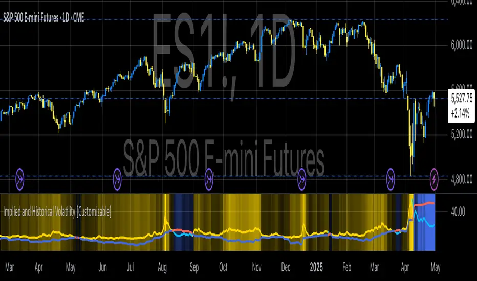
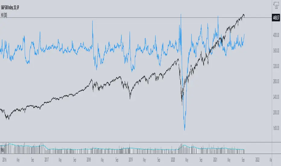
Implied and Historical VolatilityAbstract
This TradingView indicator visualizes implied volatility (IV) derived from the VIX index and historical volatility (HV) computed from past price data of the S&P 500 (or any selected asset). It enables users to compare market participants' forward-looking volatility expectations (via VIX) with realized past volatility (via historical returns). Such comparisons are pivotal in identifying risk sentiment, volatility regimes, and potential mispricing in derivatives.
Functionality
Implied Volatility (IV):
The implied volatility is extracted from the VIX index, often referred to as the "fear gauge." The VIX represents the market's expectation of 30-day forward volatility, derived from options pricing on the S&P 500. Higher values of VIX indicate increased uncertainty and risk aversion (Whaley, 2000).
Historical Volatility (HV):
The historical volatility is calculated using the standard deviation of logarithmic returns over a user-defined period (default: 20 trading days). The result is annualized using a scaling factor (default: 252 trading days). Historical volatility represents the asset's past price fluctuation intensity, often used as a benchmark for realized risk (Hull, 2018).
Dynamic Background Visualization:
A dynamic background is used to highlight the relationship between IV and HV:
Yellow background: Implied volatility exceeds historical volatility, signaling elevated market expectations relative to past realized risk.
Blue background: Historical volatility exceeds implied volatility, suggesting the market might be underestimating future uncertainty.
Use Cases
Options Pricing and Trading:
The disparity between IV and HV provides insights into whether options are over- or underpriced. For example, when IV is significantly higher than HV, options traders might consider selling volatility-based derivatives to capitalize on elevated premiums (Natenberg, 1994).
Market Sentiment Analysis:
Implied volatility is often used as a proxy for market sentiment. Comparing IV to HV can help identify whether the market is overly optimistic or pessimistic about future risks.
Risk Management:
Institutional and retail investors alike use volatility measures to adjust portfolio risk exposure. Periods of high implied or historical volatility might necessitate rebalancing strategies to mitigate potential drawdowns (Campbell et al., 2001).
Volatility Trading Strategies:
Traders employing volatility arbitrage can benefit from understanding the IV/HV relationship. Strategies such as "long gamma" positions (buying options when IV < HV) or "short gamma" (selling options when IV > HV) are directly informed by these metrics.
Scientific Basis
The indicator leverages established financial principles:
Implied Volatility: Derived from the Black-Scholes-Merton model, implied volatility reflects the market's aggregate expectation of future price fluctuations (Black & Scholes, 1973).
Historical Volatility: Computed as the realized standard deviation of asset returns, historical volatility measures the intensity of past price movements, forming the basis for risk quantification (Jorion, 2007).
Behavioral Implications: IV often deviates from HV due to behavioral biases such as risk aversion and herding, creating opportunities for arbitrage (Baker & Wurgler, 2007).
Practical Considerations
Input Flexibility: Users can modify the length of the HV calculation and the annualization factor to suit specific markets or instruments.
Market Selection: The default ticker for implied volatility is the VIX (CBOE:VIX), but other volatility indices can be substituted for assets outside the S&P 500.
Data Frequency: This indicator is most effective on daily charts, as VIX data typically updates at a daily frequency.
Limitations
Implied volatility reflects the market's consensus but does not guarantee future accuracy, as it is subject to rapid adjustments based on news or events.
Historical volatility assumes a stationary distribution of returns, which might not hold during structural breaks or crises (Engle, 1982).
References
Black, F., & Scholes, M. (1973). "The Pricing of Options and Corporate Liabilities." Journal of Political Economy, 81(3), 637-654.
Whaley, R. E. (2000). "The Investor Fear Gauge." The Journal of Portfolio Management, 26(3), 12-17.
Hull, J. C. (2018). Options, Futures, and Other Derivatives. Pearson Education.
Natenberg, S. (1994). Option Volatility and Pricing: Advanced Trading Strategies and Techniques. McGraw-Hill.
Campbell, J. Y., Lo, A. W., & MacKinlay, A. C. (2001). The Econometrics of Financial Markets. Princeton University Press.
Jorion, P. (2007). Value at Risk: The New Benchmark for Managing Financial Risk. McGraw-Hill.
Baker, M., & Wurgler, J. (2007). "Investor Sentiment in the Stock Market." Journal of Economic Perspectives, 21(2), 129-151.
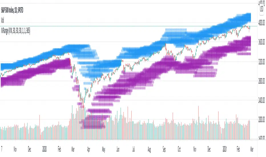
Implied Volatility LevelsOverview:
The Implied Volatility Levels Indicator is a powerful tool designed to visualize different levels of implied volatility on your trading chart. This indicator calculates various implied volatility levels based on historical price data and plots them as dynamic dotted lines, helping traders identify significant market thresholds and potential reversal points.
Features:
Multi-Level Implied Volatility: The indicator calculates and plots multiple levels of implied volatility, including the mean and both positive and negative standard deviation multiples.
Dynamic Updates: The levels update in real-time, reflecting the latest market conditions without cluttering your chart with outdated information.
Customizable Parameters: Users can adjust the lookback period and the standard deviation multiplier to tailor the indicator to their trading strategy.
Visual Clarity: Implied volatility levels are displayed using distinct colors and dotted lines, providing clear visual cues without obstructing the view of price action.
Support for Multiple Levels: Includes additional levels (up to ±5 standard deviations) for in-depth market analysis.
How It Works:
The indicator computes the standard deviation of the closing prices over a user-defined lookback period. It then calculates various implied volatility levels by adding and subtracting multiples of this standard deviation from the mean price. These levels are plotted as dotted lines on the chart, offering traders a clear view of the current market's volatility landscape.
Usage:
Identify Key Levels: Use the plotted lines to spot potential support and resistance levels based on implied volatility.
Analyze Market Volatility: Understand how volatile the market is relative to historical data.
Plan Entry and Exit Points: Make informed trading decisions by observing where the price is in relation to the implied volatility levels.
Parameters:
Lookback Period (Days): The number of days to consider for calculating historical volatility (default is 252 days).
Standard Deviation Multiplier: A multiplier to adjust the distance of the levels from the mean (default is 1.0).
This indicator is ideal for traders looking to incorporate volatility analysis into their technical strategy, providing a robust framework for anticipating market movements and potential reversals.
Implied Volatility WallsThe Implied Volatility Walls (IVW) indicator is a powerful and advanced trading tool designed to help traders identify key market zones where price may encounter significant resistance or support based on volatility. Using implied volatility, historical volatility, and machine learning models, IVW provides traders with a comprehensive understanding of market dynamics. This indicator is especially useful for those who wish to forecast volatility-driven price movements and adjust their trading strategies accordingly.
How the Implied Volatility Walls (IVW) Works:
The Implied Volatility Walls (IVW) indicator uses a combination of historical price data and advanced machine learning algorithms to calculate key volatility levels and forecast future market conditions. It tracks cumulative volatility, identifies support and resistance zones, and detects liquidation bubbles to highlight critical price areas.
The main concept behind this tool is that price tends to move most of the time by the same amount, making it possible to average the past maximum excursion in order to obtain a validated area where traders can be able to see clearly that the price is moving more than normal.
This indicator primarily focuses on:
1. Volatility Zones: Potential support and resistance levels based on implied and historical volatility.
2. Machine Learning Volatility Forecast: A machine learning model that predicts high, medium, or low volatility for future market conditions.
3. Liquidation Detection: Highlights key areas of potential forced liquidations, where market participants may be forced out of their positions, often leading to significant price movements.
4. Backtesting and Win Rate: The indicator continuously monitors how effective its volatility-based predictions are, offering insights into the performance of its predictions.
Key Features:
1. Volatility Tracking:
- The IVW indicator calculates cumulative volatility by analyzing the range between the high and low prices over time. It also tracks volatility percentiles and separates the market conditions into high, medium, or low volatility zones, enabling traders to gauge how volatile the market is.
2. Volatility Walls (Upper and Lower Zones):
- Upper Volatility Wall (Red Zones): Represent resistance levels where the price might encounter difficulty moving higher due to excess in volatility. This zone is calculated based on the chosen percentile in the settings.
- Lower Volatility Wall (Blue Zones): Represent support levels where price may find buying support.
- These walls help traders visualize potential zones where reversals or breakouts could occur based on volatility conditions.
3. Machine Learning Forecast:
- One of the standout features of the IVW indicator is its machine learning algorithm that estimates future volatility levels. It categorizes volatility into high, medium, and low based on recent data and provides forecasts on what the next market condition is likely to be.
- This forecast helps traders anticipate market conditions and adapt their strategies accordingly. It is displayed on the chart as "Exp. Vol", providing insight into the future expected volatility.
4. VIX Adjustments:
- The indicator can be adjusted using the well-known **VIX (Volatility Index)** to further refine its volatility predictions. This enables traders to incorporate market sentiment into their analysis, improving the accuracy of the predictions for different market conditions.
5. Liquidation Bubbles:
- The Liquidation Bubbles feature highlights areas where large forced selling or buying events may occur, which are usually accompanied by spikes in volatility and volume. These bubbles appear when price deviates significantly from moving averages with substantial volume increases, alerting traders to potential volatile moves.
- Red dots indicate likely forced liquidations on the upside, and blue dots indicate forced liquidations on the downside. These bubbles can help traders spot moments of market stress and potential price swings due to liquidations.
6. Dynamic Volatility Zones:
- IVW dynamically adjusts support and resistance levels as market conditions evolve. This allows traders to always have up-to-date and relevant information based on the latest volatility patterns.
7. Cumulative Volatility Histogram:
- At the bottom of the chart, the purple histogram represents cumulative volatility over time, giving traders a visual cue of whether volatility is building up or subsiding. This can provide early signals of market transitions from low to high volatility, aiding traders in timing their entries and exits more accurately.
8. Backtesting and Win Rate:
- The IVW indicator includes a backtesting function that monitors the success of its volatility predictions over a selected period. It shows a Win Rate (WR) percentage (with 33% meaning that the machine learning algorithm does not bring any edge), representing how often the indicator's predictions were correct. This metric is crucial for assessing the reliability of the model’s forecasts.
9. Opening Range:
- At the beginning of a new session, the indicator will plot two lines indicating the high and the low of the first candle of the new time frame chosen.
Chart Breakdown:
Below is a description of what users see when using the Implied Volatility Walls (IVW) indicator on the chart:
Volatility Walls:
- Red shaded zones at the top represent upper volatility walls (resistance zones), while blue shaded zones at the bottom represent lower volatility walls (support zones). These areas show where price is likely to react due to high or low volatility conditions.
Liquidation Bubbles:
- Red and blue dots plotted above and below the price represent **liquidation bubbles**, indicating moments of market stress where volatility and volume spikes may force market participants to exit positions.
Cumulative Volatility Histogram:
- The purple histogram at the bottom of the chart reflects the buildup of cumulative volatility over time. Higher bars suggest increased volatility, signaling the potential for large price movements, while smaller bars represent calmer market conditions.
Real-Time Support and Resistance Levels:
- Solid and dashed lines represent current and historical support and resistance levels, helping traders identify price zones that have historically acted as volatility-driven turning points.
Gradient Bar Colors:
- The price bars change color based on their proximity to the volatility walls, with different colors representing how close the price is to these key levels. This color gradient provides a quick visual cue of potential market turning points.
Data Tables Explained:
Table 1: **Volatility Information Table (Top Right Corner):
- EV: Expected Volatility (based on the VIX FIX calculation from Larry Williams).
- +V and -V: Represents the adjusted volatility for upward (+V) and downward (-V) movements.
- Exp. Vol: Shows the expected volatility condition for the next period (High, Medium, or Low) based on the machine learning algorithm.
- WR: The Win Rate based on the backtesting of previous volatility predictions (three outcomes, so base Win rate is 33%, and not 50%).
Table 2: Expected Cumulative Range (Top Right Corner of the separated pane):
- Exp. CR: Expected Cumulative Range based on a machine learning algorithm that calculate the most likely outcome (cumulative range) based on the past days and metrics.
How to Use the Indicator:
1. Identify Key Support and Resistance Levels:
- Use the upper (red) and lower (blue) volatility walls to identify zones where the price is likely to face resistance or support due to volatility dynamics.
2. Forecast Future Volatility:
- Pay attention to the Expected Vol field in the table to understand whether the machine learning model predicts high, medium, or low volatility for the next trading session.
3. Monitor Liquidation Bubbles:
- Watch for red and blue bubbles as they can signal significant market events where volatility and volume spikes may lead to sudden price reversals or continuations.
4. Use the Histogram to Gauge Market Conditions:
- The cumulative volatility histogram shows whether the market is entering a high or low volatility phase, helping you adjust your risk accordingly and making you able to identify the potential of the rest of the chosen session.
5. Backtesting Confidence:
- The Win Rate (WR) provides insight into how reliable the indicator’s predictions have been over the backtested period, giving you additional confidence in its future forecasts, remember that considering the 3 scenarios possible (high volatility, medium and low volatility), the standard win rate is 33%, and not 50%!.
Final Notes:
The Implied Volatility Walls (IVW) indicator is a powerful tool for volatility-based analysis, providing traders with real-time data on potential support and resistance levels, liquidation bubbles, and future market conditions. By leveraging a machine learning model for volatility forecasting, this tool helps traders stay ahead of the market’s volatility patterns and make informed decisions.
Disclaimer: This tool is for educational purposes only and should not be solely relied upon for trading decisions. Always perform your own research and risk management when trading.

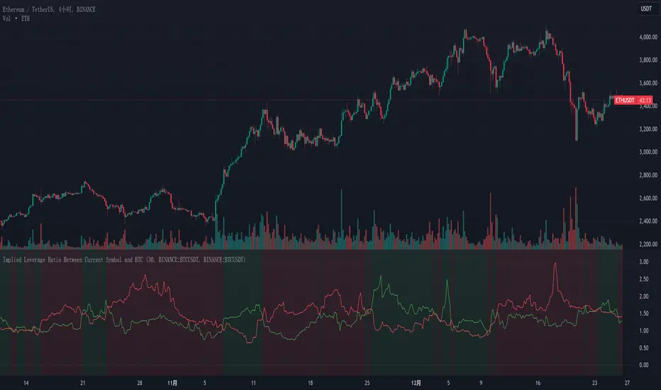
Implied Leverage Ratio Between Current Symbol and BTCThis script calculates and visualizes the implied leverage ratio between the current symbol and Bitcoin (BTC). The implied leverage ratio is computed by comparing the cumulative price changes of the two symbols over a defined number of candles. The results provide insights into how the current symbol performs relative to BTC in terms of bullish (upward) and bearish (downward) movements.
Features
Cumulative Up and Down Ratios:
The script calculates the cumulative price increase (up) and decrease (down) ratios for both the current symbol and BTC. These ratios are based on the percentage changes relative to each candle's opening price.
Implied Leverage Ratio:
For bullish movements, the cumulative up ratio of the current symbol is divided by BTC's cumulative up ratio.
For bearish movements, the cumulative down ratio of the current symbol is divided by BTC's cumulative down ratio.
These values reflect the implied leverage of the current symbol relative to BTC in both directions.
Customizable Comparison Symbol:
By default, the script compares the current symbol to BINANCE:BTCUSDT. However, you can specify any other symbol to tailor the analysis.
Interactive Visualization:
Green Line: Represents the ratio of cumulative up movements (current symbol vs. BTC).
Red Line: Represents the ratio of cumulative down movements (current symbol vs. BTC).
A horizontal zero line is included for reference, ensuring the chart always starts from zero.
How to Use
Add this script to your chart from the Pine Editor or the public library.
Customize the number of candles (t) to define the period over which cumulative changes are calculated.
If desired, replace the comparison symbol with another asset in the input settings.
Analyze the green and red lines to identify relative strength and implied leverage trends.
Who Can Benefit
Traders and Analysts: Gain insights into the relative performance of altcoins, stocks, or other instruments against BTC.
Leverage Seekers: Identify assets with higher or lower implied leverage compared to Bitcoin.
Market Comparisons: Understand how various assets react to market movements relative to BTC.
This tool is particularly useful for identifying potential outperformers or underperformers relative to Bitcoin and can guide strategic decisions in trading pairs or market analysis.
Implied Volatility and Historical VolatilityThis indicator provides a visualization of two different volatility measures, aiding in understanding market perceptions and actual price movements. Remember to combine it with other technical analysis tools and risk management strategies for informed trading decisions. The two measures of volatility:
Implied Volatility: Based on the standard deviation of recent price changes, it represents the market's expectation of future volatility.
Historical Volatility: Measured by the daily high-low range as a percentage of the closing price, it reflects the actual volatility experienced recently. It is intended to be used along side the Mean and Standard Deviation Lines indicator.
Inputs:
Period (Days): Defines the number of past bars used to calculate both types of volatility.
Calculations:
Interpretation:
Comparing the lines: Divergence between the lines can indicate potential mispricing:
If the Implied Volatility is higher than the Historical Volatility, the market might be overestimating future volatility.
Conversely, if the Implied Volatility is lower, the market might be underestimating future volatility.
Monitoring trends: Track changes in both lines over time to identify potential shifts in volatility expectations or actual market behavior.
Limitations:
Assumes normality in price distribution, which may not always hold true.
Historical Volatility only reflects past behavior, not future expectations.
Consider other factors like market sentiment and news events for comprehensive volatility analysis.

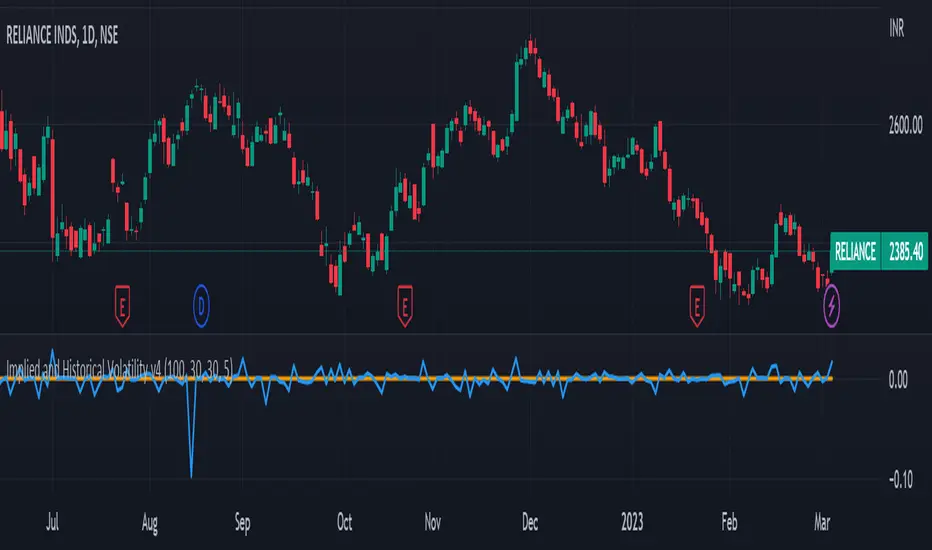
Implied and Historical Volatility v4There is a famous option strategy📊 played on volatility📈. Where people go short on volatility, generally, this strategy is used before any significant event or earnings release. The basic phenomenon is that the Implied Volatility shoots up before the event and drops after the event, while the volatility of the security does not increase in most of the scenarios. 💹
I have tried to create an Indicator using which you
can analyse the historical change in Implied Volatility Vs Historic Volatility.
To get a basic idea of how the security moved during different events.
Notes:
a) Implied Volatility is calculated using the bisection method and Black 76 model option pricing model.
b) For the risk-free rate I have fetched the price of the “10-Year Indian Government Bond” price and calculated its yield to be used as our Risk-Free rate.
Implied Volatility Range ProjectionThis script plots an expected future range estimation based on implied volatilities, using a specified volatility index as proxy for ATM implied volatilities.
For example the S&P 500 could use the VIX.
Implied minus Historical VolatilityJust a simple comparison of 30 day historical volatility versus 30 day implied volatility(VIX). In general, when VIX is way above realized or historical Vol, in general that is quite bullish. Backtest will be available soon.
Synthetic Implied APROverview
The Synthetic Implied APR is an artificial implied APR, designed to imitate the implied APR seen when trading cryptocurrency funding rates. It combines real-time funding rates with premium data to calculate an artificial market expectation of the annualized funding rate.
The (actual) implied APR is the market's expectation of the annualized funding rate. This is dependent on bid/ask impacts of the implied APR, something which is currently unavailable to fetch with TradingView. In essence, an implied APR of X% means traders believe that asset's funding fees to average X% when annualized.
What's important to understand, is that the actual value of the synthetic implied APR is not relevant. We only simply use its relative changes when we trade (i.e if it crosses above/below its MA for a given weight). Even for the same asset, the implied APRs will change depending on days to maturity.
How it calculates
The synthetic implied APR is calculated with these steps:
Collects premium data from perpetual futures markets using optimized lower timeframe requests (check my 'Predicted Funding Rates' indicator)
Calculates the funding rate by adding the premium to an interest rate component (clamped within exchange limits)
Derives the underlying APR from the 8-hour funding rate (funding rate × 3 × 365)
Apply a weighed formula that imitates both the direction (underlying APR) with the volatility of prices (from the premium index and funding)
premium_component = (prem_avg / 50 ) * 365
weighedprem = (weight * fr) + ((1 - weight) * apr) + (premium_component * 0.3)
impliedAPR = math.avg(weighedprem, ta.sma(apr, maLength))
How to use it: Generally
Preface: Funding rates are an indication of market sentiment
If funding is positive, generally the market is bullish as longs are willing to pay shorts funding
If funding is negative, generally the market is bearish as shorts are willing to pay longs funding
So, this script can be used like a typical oscillator:
Bullish: If implied APR > MA OR if implied APR MA is green
Bearish: If implied APR < MA OR if implied APR MA is red
The components:
Synthetic Implied APR: The main metric. At current setting of 0.7, it imitates volatility
Weight: The higher the value, the smoother the synthetic implied APR is (and MA too). This value is very important to the imitation. At 0.7, it imitates the actual volatility of the implied APR. At weight = 1, it becomes very smooth. Perfect for trading
Synthetic Implied APR Moving Average: A moving average of the Synthetic implied APR. Can choose from multiple selections, (SMA, EMA, WMA, HMA, VWMA, RMA)
How to use it: Trading Funding
When trading funding there're multiple ways to use it with different settings
Trade funding rates with trend changes
Settings: Weight = 1
Method 1: When the implied APR MA turns green, long funding rates (or short if red)
Method 2: When the implied APR crosses above the MA, long funding rates (or short when crosses below)
Trade funding rates with MA pullbacks
Settings: Weight = 0.7, timeframe 15m
In an uptrend: When implied APR crosses below then above the script, long funding opportunity
In an downtrend: When implied APR crosses above then below the script, shortfunding opportunity
You can determine the trend with the method before, using a weight of 1
To trade funding rates, it's best to have these 3 scripts at these settings:
Predicted Funding Rates: This allows you to see the predicted funding rates and see if they've maxxed out for added confluence too (+/-0.01% usually for Binance BTC futures)
Synthetic implied APR: At weight 1, the MA provides a good trend (whether close above/below or colour change)
Synthetic implied APR: At weight 0.7, it provides a good imitation of volatility
How to use it: Trading Futures
When trading futures:
You can determine roughly what the trend is, if the assumption is made that funding rates can help identify trends if used as a sentiment indicator. It should be supplemented with traditional trend trading methods
To prevent whipsaws, weight should remain high
Long trend: When the implied APR MA turns green OR when it crosses above its MA
Short trend: When the implied APR MA turns red OR when it below above its MA
Why it's original
This indicator introduces a unique synthetic weighting system that combines funding rates, underlying APR, and premium components in a way not found in existing TradingView scripts. Trading funding rates is a niche area, there aren't that many scripts currently available. And to my knowledge, there's no synthetic implied APR scripts available on TradingView either. So I believe this script to be original in that sense.
Notes
Because it depends on my triangular weighting algos, optimal accuracy is found on timeframes that are 4H or less. On higher timeframes, the accuracy drops off. Best timeframes for intraday trading using this are 15m or 1 hour
The higher the timeframe, the lower the MA one should use. At 1 hour, 200 or higher is best. At say, 4h, length of 50 is best
Only works for coins that have a Binance premium index
Inputs
Funding Period - Select between "1 Hour" or "8 Hour" funding cycles. 8 hours is standard for Binance
Table - Toggle the information dashboard on/off to show or hide real-time metrics including funding rate, premium, and APR value
Weight - Controls the balance between funding rate (higher values = smoother) and APR (lower values = more responsive) in the calculation, ranging from 0.0 to 1.0. Default is 0.7, this imitates the volatility
Auto Timeframe Implied Length - Automatically calculates optimal smoothing length based on your chart timeframe for consistent behavior across different time periods
Manual Implied Length - Sets a fixed smoothing length (in bars) when auto mode is disabled, with lower values being more responsive and higher values being smoother
Show Implied APR MA - Displays an additional moving average line of the Synthetic Implied APR to help identify trend direction and crossover signals
MA Type for Implied APR - Selects the calculation method (SMA, EMA, WMA, HMA, VWMA, or RMA) for the moving average, each offering different responsiveness and lag characteristics
MA Length for Implied APR - Sets the lookback period (1-500 bars) for the moving average, with shorter lengths providing more signals and longer lengths filtering noise
Show Underlying APR - Displays the raw APR calculation (without synthetic weighting) as a reference line to compare against the main indicator
Bullish Color - Sets the color for positive values in the table and rising MA line
Bearish Color - Sets the color for negative values in the table and falling MA line
Table Background - Customizes the background color and transparency of the information dashboard
Table Text Color - Sets the color for label text in the left column of the information table
Table Text Size - Controls the font size of table text with options from Tiny to Huge

Options Overlay [Pro] IVR IV Skew Delta Exp.mv MurreyMath Expiry
𝗧𝗵𝗲 𝗳𝗶𝗿𝘀𝘁 𝗿𝗲𝗮𝗹 𝗼𝗽𝘁𝗶𝗼𝗻𝘀 𝗱𝗮𝘁𝗮 𝗶𝗻𝗱𝗶𝗰𝗮𝘁𝗼𝗿 𝗼𝗻 𝗧𝗿𝗮𝗱𝗶𝗻𝗴𝗩𝗶𝗲𝘄, 𝗮𝘃𝗮𝗶𝗹𝗮𝗯𝗹𝗲 𝗳𝗼𝗿 𝗼𝘃𝗲𝗿 𝟭𝟱𝟬+ 𝗹𝗶𝗾𝘂𝗶𝗱 𝗨𝗦 𝗺𝗮𝗿𝗸𝗲𝘁 𝘀𝘆𝗺𝗯𝗼𝗹𝘀.
🔃 Auto-Updating Option Metrics without refresh!
🍒 Developed and maintained by option traders for option traders.
📈 Specifically designed for TradingView users who trade options.
Our indicator provides essential key metrics such as:
✅ IVRank
✅ IVx
✅ 5-Day IVx Change
✅ Delta curves and interpolated distances
✅ Expected move curve
✅ Standard deviation (STD1) curve
✅ Vertical Pricing Skew
✅ Horizontal IVx Skew
✅ Delta Skew
like TastyTrade, TOS, IBKR etc, but in a much more visually intuitive way. See detailed descriptions below.
If this isn't enough, we also include a unique grid system designed specifically for options traders. This package features our innovative dynamic grid system:
✅ Enhanced Murrey Math levels (horizontal scale)
✅ Options expirations (vertical scale)
Designed to help you assess market conditions and make well-informed trading decisions, this tool is an essential addition for every serious options trader!
Ticker Information:
This indicator is currently implemented for more than 150 liquid US market tickers and we are continuously expanding the list:
SP:SPX AMEX:SPY NASDAQ:QQQ NASDAQ:TLT AMEX:GLD
NYSE:AA NASDAQ:AAL NASDAQ:AAPL NYSE:ABBV NASDAQ:ABNB NASDAQ:AMD NASDAQ:AMZN AMEX:ARKK NASDAQ:AVGO NYSE:AXP NYSE:BA NYSE:BABA NYSE:BAC NASDAQ:BIDU AMEX:BITO NYSE:BMY NYSE:BP NASDAQ:BYND NYSE:C NYSE:CAT NYSE:CCJ NYSE:CCL NASDAQ:COIN NYSE:COP NASDAQ:COST NYSE:CRM NASDAQ:CRWD NASDAQ:CSCO NYSE:CVNA NYSE:CVS NYSE:CVX NYSE:DAL NASDAQ:DBX AMEX:DIA NYSE:DIS NASDAQ:DKNG NASDAQ:EBAY NASDAQ:ETSY NASDAQ:EXPE NYSE:F NYSE:FCX NYSE:FDX AMEX:FXI AMEX:GDX AMEX:GDXJ NYSE:GE NYSE:GM NYSE:GME NYSE:GOLD NASDAQ:GOOG NASDAQ:GOOGL NYSE:GPS NYSE:GS NASDAQ:HOOD NYSE:IBM NASDAQ:IEF NASDAQ:INTC AMEX:IWM NASDAQ:JD NYSE:JNJ NYSE:JPM NYSE:JWN NYSE:KO NYSE:LLY NYSE:LOW NYSE:LVS NYSE:MA NASDAQ:MARA NYSE:MCD NYSE:MET NASDAQ:META NYSE:MGM NYSE:MMM NYSE:MPC NYSE:MRK NASDAQ:MRNA NYSE:MRO NASDAQ:MRVL NYSE:MS NASDAQ:MSFT AMEX:MSOS NYSE:NCLH NASDAQ:NDX NYSE:NET NASDAQ:NFLX NYSE:NIO NYSE:NKE NASDAQ:NVDA NASDAQ:ON NYSE:ORCL NYSE:OXY NASDAQ:PEP NYSE:PFE NYSE:PINS NYSE:PLTR NASDAQ:PTON NASDAQ:PYPL NASDAQ:QCOM NYSE:RBLX NYSE:RCL NASDAQ:RIOT NASDAQ:RIVN NASDAQ:ROKU NASDAQ:SBUX NYSE:SHOP AMEX:SLV NASDAQ:SMCI NASDAQ:SMH NYSE:SNAP NYSE:SQ NYSE:T NYSE:TGT NASDAQ:TQQQ NASDAQ:TSLA NYSE:TSM NASDAQ:TTD NASDAQ:TXN NYSE:U NASDAQ:UAL NYSE:UBER AMEX:UNG NYSE:UPS NASDAQ:UPST AMEX:USO NYSE:V AMEX:VXX NYSE:VZ NASDAQ:WBA NYSE:WFC NYSE:WMT NASDAQ:WYNN NYSE:X AMEX:XHB AMEX:XLE AMEX:XLF AMEX:XLI AMEX:XLK AMEX:XLP AMEX:XLU AMEX:XLV AMEX:XLY NYSE:XOM NYSE:XPEV CBOE:XSP NASDAQ:ZM
How does the indicator work and why is it unique?
This Pine Script indicator is a complex tool designed to provide various option metrics and visualization tools for options market traders. The indicator extracts raw options data from an external data provider (ORATS), processes and refines the delayed data package using pineseed, and sends it to TradingView, visualizing the data using specific formulas (see detailed below) or interpolated values (e.g., delta distances). This method of incorporating options data into a visualization framework is unique and entirely innovative on TradingView.
The indicator aims to offer a comprehensive view of the current state of options for the implemented instruments, including implied volatility (IV), IV rank (IVR), options skew, and expected market movements, which are objectively measured as detailed below.
The options metrics we display may be familiar to options traders from various major brokerage platforms such as TastyTrade, IBKR, TOS, Tradier, TD Ameritrade, Schwab, etc.
🟨 𝗗𝗘𝗧𝗔𝗜𝗟𝗘𝗗 𝗗𝗢𝗖𝗨𝗠𝗘𝗡𝗧𝗔𝗧𝗜𝗢𝗡 🟨
🔶 Auto-Updating Option Metrics and Curved Lines
🔹 Interpolated DELTA Curves (16,20,25,30,40)
In our indicator, the curve layer settings allow you to choose the delta value for displaying the delta curve: 16, 20, 25, 30, or even 40. The color of the curve can be customized, and you can also hide the delta curve by selecting the "-" option.
It's important to mention that we display interpolated deltas from the actual option chain of the underlying asset using the Black-Scholes model. This ensures that the 16 delta truly reflects the theoretical, but accurate, 16 delta distance. (For example, deltas shown by brokerages for individual strikes are rounded; a 0.16 delta might actually be 0.1625.)
🔹 Expected Move Curve (Exp.mv)
The expected move is the predicted dollar change in the underlying stock's price by a given option's expiration date, with 68% certainty. It is calculated using the expiration's pricing and implied volatility levels. We chose the TastyTrade method for calculating expected move, as we found it to be the most expressive.
Expected Move Calculation
Expected Move = (ATM straddle price x 0.6) + (1st OTM strangle price x 0.3) + (2nd OTM strangle price x 0.1)
For example , if stock XYZ is trading at 121 and the ATM straddle is 4.40, the 120/122 strangle is 3.46, and the 119/123 strangle is 2.66, the expected move is calculated as follows: 4.40 x 0.60 = 2.64; 3.46 x 0.30 = 1.04; 2.66 x 0.10 = 0.27; Expected move = 2.64 + 1.04 + 0.27 = ±3.9
In this example below, the TastyTrade platform indicates the expected move on the option chain with a brown color, and the exact value is displayed behind the ± symbol for each expiration. By default, we also use brown for this indication, but this can be changed or the curve display can be turned off.
🔹 Standard Deviation Curve (1 STD)
One standard deviation of a stock encompasses approximately 68.2% of outcomes in a distribution of occurrences based on current implied volatility.
We use the expected move formula to calculate the one standard deviation range of a stock. This calculation is based on the days-to-expiration (DTE) of our option contract, the stock price, and the implied volatility of a stock:
Calculation:
Standard Deviation = Closing Price * Implied Volatility * sqrt(Days to Expiration / 365)
According to options literature, there is a 68% probability that the underlying asset will fall within this one standard deviation range at expiration.
If the 1 STD and Exp.mv displays are both enabled, the indicator fills the area between them with a light gray color. This is because both represent probability distributions that appear as a "bell curve" when graphed, making it visually appealing.
Tip and Note:
The 1 STD line might appear jagged at times , which does not indicate a problem with the indicator. This is normal immediately after market open (e.g., during the first data refresh of the day) or if the expirations are illiquid (e.g., weekly expirations). The 1 STD value is calculated based on the aggregated IVx for the expirations, and the aggregated IVx value for weekly expirations updates less frequently due to lower trading volume. In such cases, we recommend enabling the "Only Monthly Expirations" option to smooth out the bell curve.
∑ Quant Observation:
The values of the expected move and the 1st standard deviation (1STD) will not match because they use different calculation methods, even though both are referred to as representing 68% of the underlying asset's movement in options literature. The expected move is based on direct market pricing of ATM options. The 1STD, on the other hand, uses the averaged implied volatility (IVX) for the given expiration to determine its value. Based on our experience, it is better to consider the area between the expected move and the 1STD as the true representation of the original 68% rule.
🔶 IVR Dashboard Panel Rows
🔹 IVR (IV Rank)
The Implied Volatility Rank (IVR) indicator helps options traders assess the current level of implied volatility (IV) in comparison to the past 52 weeks. IVR is a useful metric to determine whether options are relatively cheap or expensive. This can guide traders on whether to buy or sell options. We calculate IVrank, like TastyTrade does.
IVR Calculation:
IV Rank = (current IV - 52 week IV low) / (52 week IV high - 52 week IV low)
IVR Levels and Interpretations:
IVR 0-10 (Green): Very low implied volatility rank. Options might be "cheap," potentially a good time to buy options.
IVR 10-35 (White): Normal implied volatility rank. Options pricing is relatively standard.
IVR 35-50 (Orange): Almost high implied volatility rank.
IVR 50-75 (Red): Definitely high implied volatility rank. Options might be "expensive," potentially a good time to sell options for higher premiums.
IVR above 75 (Highlighted Red): Ultra high implied volatility rank. Indicates very high levels, suggesting a favorable time for selling options.
The panel refreshes automatically if the symbol is implemented. You can hide the panel or change the position and size.
🔹IVx (Implied Volatility Index)
The Implied Volatility Index (IVx) displayed in the option chain is calculated similarly to the VIX. The Cboe uses standard and weekly SPX options to measure the expected volatility of the S&P 500. A similar method is utilized to calculate IVx for each option expiration cycle.
For our purposes on the IVR Panel, we aggregate the IVx values specifically for the 35-70 day monthly expiration cycle . This aggregated value is then presented in the screener and info panel, providing a clear and concise measure of implied volatility over this period.
IVx Color coding:
IVx above 30 is displayed in orange.
IVx above 60 is displayed in red
IVx on curve:
The IVx values for each expiration can be viewed by hovering the mouse over the colored tooltip labels above the Curve.
IVx avg on IVR panel :
If the option is checked in the IVR panel settings, the IVR panel will display the average IVx values up to the optimal expiration.
Important Note:
The IVx value alone does not provide sufficient context. There are stocks that inherently exhibit high IVx values. Therefore, it is crucial to consider IVx in conjunction with the Implied Volatility Rank (IVR), which measures the IVx relative to its own historical values. This combined view helps in accurately assessing the significance of the IVx in relation to the specific stock's typical volatility behavior.
This indicator offers traders a comprehensive view of implied volatility, assisting them in making informed decisions by highlighting both the absolute and relative volatility measures.
🔹IVx 5 days change %
We are displaying the five-day change of the IV Index (IVx value). The IV Index 5-Day Change column provides quick insight into recent expansions or decreases in implied volatility over the last five trading days.
Traders who expect the value of options to decrease might view a decrease in IVX as a positive signal. Strategies such as Strangle and Ratio Spread can benefit from this decrease.
On the other hand, traders anticipating further increases in IVX will focus on the rising IVX values. Strategies like Calendar Spread or Diagonal Spread can take advantage of increasing implied volatility.
This indicator helps traders quickly assess changes in implied volatility, enabling them to make informed decisions based on their trading strategies and market expectations.
🔹 Vertical Pricing Skew
At TanukiTrade, Vertical Pricing Skew refers to the difference in pricing between put and call options with the same expiration date at the same distance (at expected move). We analyze this skew to understand market sentiment. This is the same formula used by TastyTrade for calculations.
We calculate the interpolated strike price based on the expected move , taking into account the neighboring option prices and their distances. This allows us to accurately determine whether the CALL or PUT options are more expensive.
PUT Skew (red): Put options are more expensive than call options, indicating the market expects a downward move (▽). If put options are more expensive by more than 20% at the same expected move distance, we color it lighter red.
CALL Skew (green): Call options are more expensive than put options, indicating the market expects an upward move (△). If call options are priced more than 30% higher at the examined expiration, we color it lighter green.
Vertical Skew on Curve:
The degree of vertical pricing skew for each expiration can be viewed by hovering over the points above the curve. Hover with mouse for more information.
Vertical Skew on IVR panel:
We focus on options with 35-70 days to expiration (DTE) for optimal analysis in case of vertical skew. Hover with mouse for more information.
This approach helps us gauge market expectations accurately, providing insights into potential price movements. Remember, we always evaluate the skew at the expected move using linear interpolation to determine the theoretical pricing of options.
🔹 Delta Skew 🌪️ (Twist)
We have a new metric that examines which monthly expiration indicates a "Delta Skew Twist" where the 16 delta deviates from the monthly STD. This is important because, under normal circumstances, the 16 delta is positioned between the expected move and the standard deviation (STD1) line (see Exp.mv & 1STD exact definitions above). However, if the interpolated 16 delta line exceeds the STD1 line either upwards or downwards, it represents a special case of vertical skew on the option chain.
Normal case : exp.move < delta16 < std1
Delta Skew Twist: exp.move < std1 < delta16
We indicate this with direction-specific colors (red/green) on the delta line. We also color the section of the delta curve affected by the delta skew in this case, even if you choose to display a lower delta, such as 30, instead of 16.
If "Colored Labels with Tooltips" is enabled, we also display a 🌪️ symbol in the tooltip for the expirations affected by Delta Skew.
If you have enabled the display of 'Vertical Pricing Skew' on the IVR Panel, a 🌪️ symbol will also appear next to the value of the vertical skew, and the tooltip will indicate from which expiration Delta Skew is observed.
🔹 Horizontal IVx Skew
In options pricing, it is typically expected that the implied volatility (IVx) increases for options with later expiration dates. This means that options further out in time are generally more expensive. At TanukiTrade, we refer to the phenomenon where this expectation is reversed—when the IVx decreases between two consecutive expirations—as Horizontal Skew or IVx Skew.
Horizontal IVx Skew occurs when: Front Expiry IVx < Back Expiry IVx
This scenario can create opportunities for traders who prefer diagonal or calendar strategies . Based on our experience, we categorize Horizontal Skew into two types:
Weekly Horizontal Skew:
When IVx skew is observed between two consecutive non-monthly expirations, the displayed value is the rounded-up percentage difference. On hover, the approximate location of this skew is also displayed. The precise location can be seen on this indicator.
Monthly Horizontal Skew:
When IVx skew is observed between two consecutive monthly expirations , the displayed value is the rounded-up percentage difference. On hover, the approximate location of this skew is also displayed. The precise location can be seen on our Overlay indicator.
The Monthly Vertical IVx skew is consistently more liquid than the weekly vertical IVx skew. Weekly Horizontal IVx Skew may not carry relevant information for symbols not included in the 'Weeklies & Volume Masters' preset in our Options Screener indicator.
If the options chain follows the normal IVx pattern, no skew value is displayed.
Color codes or tooltip labels above curve:
Gray - No horizontal skew;
Purple - Weekly horizontal skew;
BigBlue - Monthly horizontal skew
The display of monthly and weekly IVx skew can be toggled on or off on the IVR panel. However, if you want to disable the colored tooltips above the curve, this can only be done using the "Colored labels with tooltips" switch.
We indicate this range with colorful information bubbles above the upper STD line.
🔶 The Option Trader’s GRID System: Adaptive MurreyMath + Expiry Lines
At TanukiTrade, we utilize Enhanced MurreyMath and Expiry lines to create a dynamic grid system, unlike the basic built-in vertical grids in TradingView, which provide no insight into specific price levels or option expirations.
These grids are beneficial because they provide a structured layout, making important price levels visible on the chart. The grid automatically resizes as the underlying asset's volatility changes, helping traders identify expected movements for various option expirations.
The Option Trader’s GRID System part of this indicator can be used without limitations for all instruments . There are no type or other restrictions, and it automatically scales to fit every asset. Even if we haven't implemented the option metrics for a particular underlying asset, the GRID system will still function!
🔹 SETUP OF YOUR OPTIONS GRID SYSTEM
You can setup your new grid system in 3 easy steps!
STEP1: Hide default horizontal grid lines in TradingView
Right-click on an empty area of your chart, then select “Settings.” In the Chart settings -> Canvas -> Grid lines section, disable the display of horizontal lines to avoid distraction.
SETUP STEP2: Scaling fix
Right-click on the price scale on the right side, then select "Scale price chart only" to prevent the chart from scaling to the new horizontal lines!
STEP3: Enable Tanuki Options Grid
As a final step, make sure that both the vertical (MurreyMath) and horizontal (Expiry) lines are enabled in the Grid section of our indicator.
You are done, enjoy the new grid system!
🔹 HORIZONTAL: Enhanced MurreyMath Lines
Murrey Math lines are based on the principles observed by William Gann, renowned for his market symmetry forecasts. Gann's techniques, such as Gann Angles, have been adapted by Murrey to make them more accessible to ordinary investors. According to Murrey, markets often correct at specific price levels, and breakouts or returns to these levels can signal good entry points for trades.
At TanukiTrade, we enhance these price levels based on our experience , ensuring a clear display. We acknowledge that while MurreyMath lines aren't infallible predictions, they are useful for identifying likely price movements over a given period (e.g., one month) if the market trend aligns.
Our opinion: MurreyMath lines are not crystal balls (like no other tool). They should be used to identify that if we are trading in the right direction, the price is likely to reach the next unit step within a unit time (e.g. monthly expiration).
One unit step is the distance between Murrey Math lines, such as between the 0/8 and 1/8 lines. This interval helps identify different quadrants and is crucial for recognizing support and resistance levels.
Some option traders use Murrey Math lines to gauge the movement speed of an instrument over a unit time. A quadrant encompasses 4 unit steps.
Key levels, according to TanukiTrade, include:
Of course, the lines can be toggled on or off, and their default color can also be changed.
🔹 VERTICAL: Expiry Lines
The indicator can display monthly and weekly expirations as dashed lines, with customizable colors. Weekly expirations will always appear in a lighter shade compared to monthly expirations.
Monthly Expiry Lines:
You can turn off the lines indicating monthly expirations, or set the direction (past/future/both) and the number of lines to be drawn.
Weekly Expiry Lines:
You can display weekly expirations pointing to the future. You can also turn them off or specify how many weeks ahead the lines should be drawn.
Of course, the lines can be toggled on or off, and their default color can also be changed.
TIP: Hide default vertical grid lines in TradingView
Right-click on an empty area of your chart, then select “Settings.” In the Chart settings -> Canvas -> Grid lines section, disable the display of vertical lines to avoid distraction. Same, like steps above at MurreyMath lines.
🔶 ADDITIONAL IMPORTANT COMMENTS
- U.S. market only:
Since we only deal with liquid option chains: this option indicator only works for the USA options market and do not include future contracts; we have implemented each selected symbol individually.
- Why is there a slight difference between the displayed data and my live brokerage data? There are two reasons for this, and one is beyond our control.
- Brokerage Calculation Differences:
Every brokerage has slight differences in how they calculate metrics like IV and IVx. If you open three windows for TOS, TastyTrade, and IBKR side by side, you will notice that the values are minimally different. We had to choose a standard, so we use the formulas and mathematical models described by TastyTrade when analyzing the options chain and drawing conclusions.
- Option-data update frequency:
According to TradingView's regulations and guidelines, we can update external data a maximum of 5 times per day. We strive to use these updates in the most optimal way:
(1st update) 15 minutes after U.S. market open
(2nd, 3rd, 4th updates) 1.5–3 hours during U.S. market open hours
(5th update) 10 minutes before market close.
You don’t need to refresh your window, our last refreshed data-pack is always automatically applied to your indicator , and you can see the time elapsed since the last update at the bottom of your indicator.
- Skewed Curves:
The delta, expected move, and standard deviation curves also appear relevantly on a daily or intraday timeframe. Data loss is experienced above a daily timeframe: this is a TradingView limitation.
- Weekly illiquid expiries:
Especially for instruments where weekly options are illiquid: the weekly expiration STD1 data is not relevant. In these cases, we recommend checking in the "Display only Monthly labels" checkbox to avoid displaying not relevant weekly options expirations.
-Timeframe Issues:
Our option indicator visualizes relevant data on a daily resolution. If you see strange or incorrect data (e.g., when the options data was last updated), always switch to a daily (1D) timeframe. If you still see strange data, please contact us.
Disclaimer:
Our option indicator uses approximately 15min-3 hour delayed option market snapshot data to calculate the main option metrics. Exact realtime option contract prices are never displayed; only derived metrics and interpolated delta are shown to ensure accurate and consistent visualization. Due to the above, this indicator can only be used for decision support; exclusive decisions cannot be made based on this indicator . We reserve the right to make errors.This indicator is designed for options traders who understand what they are doing. It assumes that they are familiar with options and can make well-informed, independent decisions. We work with public data and are not a data provider; therefore, we do not bear any financial or other liability.

Options Screener [Pro] - IVRank, IVx, Deltas, Exp.move, Skew
𝗢𝗽𝘁𝗶𝗼𝗻 𝘀𝗰𝗿𝗲𝗲𝗻𝗲𝗿 𝗼𝗻 𝗧𝗿𝗮𝗱𝗶𝗻𝗴𝗩𝗶𝗲𝘄 𝘄𝗶𝘁𝗵 𝗿𝗲𝗮𝗹 𝗱𝗮𝘁𝗮, 𝗮𝘃𝗮𝗶𝗹𝗮𝗯𝗹𝗲 𝗳𝗼𝗿 𝗼𝘃𝗲𝗿 𝟭𝟱𝟬+ 𝗹𝗶𝗾𝘂𝗶𝗱 𝗨𝗦 𝗺𝗮𝗿𝗸𝗲𝘁 𝘀𝘆𝗺𝗯𝗼𝗹𝘀!
𝗢𝘂𝗿 𝘀𝗰𝗿𝗲𝗲𝗻𝗲𝗿 𝗽𝗿𝗼𝘃𝗶𝗱𝗲𝘀 𝗲𝘀𝘀𝗲𝗻𝘁𝗶𝗮𝗹 𝗸𝗲𝘆 𝗺𝗲𝘁𝗿𝗶𝗰𝘀 𝘀𝘂𝗰𝗵 𝗮𝘀:
✅ IVRank
✅ IVx
✅ 5-Day IVx Change
✅ Vertical Pricing Skew
✅ Horizontal IVx Skew
✅ Delta Skew
like TastyTrade, TOS, IBKR etc.
Designed to help you assess option market conditions and make well-informed trading decisions, this tool is an essential addition for every serious options trader!
Ticker Information:
This screener is currently implemented for more than 150 liquid US market tickers and we are continuously expanding the list:
SP:SPX AMEX:SPY NASDAQ:QQQ NASDAQ:TLT AMEX:GLD
NYSE:AA NASDAQ:AAL NASDAQ:AAPL NYSE:ABBV NASDAQ:ABNB NASDAQ:AMD NASDAQ:AMZN AMEX:ARKK NASDAQ:AVGO NYSE:AXP NYSE:BA NYSE:BABA NYSE:BAC NASDAQ:BIDU AMEX:BITO NYSE:BMY NYSE:BP NASDAQ:BYND NYSE:C NYSE:CAT NYSE:CCJ NYSE:CCL NASDAQ:COIN NYSE:COP NASDAQ:COST NYSE:CRM NASDAQ:CRWD NASDAQ:CSCO NYSE:CVNA NYSE:CVS NYSE:CVX NYSE:DAL NASDAQ:DBX AMEX:DIA NYSE:DIS NASDAQ:DKNG NASDAQ:EBAY NASDAQ:ETSY NASDAQ:EXPE NYSE:F NYSE:FCX NYSE:FDX AMEX:FXI AMEX:GDX AMEX:GDXJ NYSE:GE NYSE:GM NYSE:GME NYSE:GOLD NASDAQ:GOOG NASDAQ:GOOGL NYSE:GPS NYSE:GS NASDAQ:HOOD NYSE:IBM NASDAQ:IEF NASDAQ:INTC AMEX:IWM NASDAQ:JD NYSE:JNJ NYSE:JPM NYSE:JWN NYSE:KO NYSE:LLY NYSE:LOW NYSE:LVS NYSE:MA NASDAQ:MARA NYSE:MCD NYSE:MET NASDAQ:META NYSE:MGM NYSE:MMM NYSE:MPC NYSE:MRK NASDAQ:MRNA NYSE:MRO NASDAQ:MRVL NYSE:MS NASDAQ:MSFT AMEX:MSOS NYSE:NCLH NASDAQ:NDX NYSE:NET NASDAQ:NFLX NYSE:NIO NYSE:NKE NASDAQ:NVDA NASDAQ:ON NYSE:ORCL NYSE:OXY NASDAQ:PEP NYSE:PFE NYSE:PINS NYSE:PLTR NASDAQ:PTON NASDAQ:PYPL NASDAQ:QCOM NYSE:RBLX NYSE:RCL NASDAQ:RIOT NASDAQ:RIVN NASDAQ:ROKU NASDAQ:SBUX NYSE:SHOP AMEX:SLV NASDAQ:SMCI NASDAQ:SMH NYSE:SNAP NYSE:SQ NYSE:T NYSE:TGT NASDAQ:TQQQ NASDAQ:TSLA NYSE:TSM NASDAQ:TTD NASDAQ:TXN NYSE:U NASDAQ:UAL NYSE:UBER AMEX:UNG NYSE:UPS NASDAQ:UPST AMEX:USO NYSE:V AMEX:VXX NYSE:VZ NASDAQ:WBA NYSE:WFC NYSE:WMT NASDAQ:WYNN NYSE:X AMEX:XHB AMEX:XLE AMEX:XLF AMEX:XLI AMEX:XLK AMEX:XLP AMEX:XLU AMEX:XLV AMEX:XLY NYSE:XOM NYSE:XPEV CBOE:XSP NASDAQ:ZM
How does the screener work and why is it unique?
This Pine Script screener is an expert tool created to provide various option metrics and visualization tools for options market traders. The screener extracts raw options data from an external data provider (ORATS), processes, and refines the delayed data package using pineseed, and sends it to TradingView. The data is calculated using specific formulas or interpolated values, such as delta distances. This method of integrating options data into a screener framework is unique and innovative on TradingView.
The screener aims to offer a comprehensive view of the current state of options for the implemented instruments, including implied volatility index (IVx), IV rank (IVR), options skew, and expected market movements, which are objectively measured as detailed below.
The options metrics displayed may be familiar to options traders from various major brokerage platforms such as TastyTrade, IBKR, TOS, Tradier, TD Ameritrade, Schwab, etc.
🟨 𝗗𝗘𝗧𝗔𝗜𝗟𝗘𝗗 𝗗𝗢𝗖𝗨𝗠𝗘𝗡𝗧𝗔𝗧𝗜𝗢𝗡 🟨
~~~~~~~~~~~~~~~~~~~~~~~~~~~~~~~~~~~~~~~~~~~~~~~~~~
~~~~~~~~~~~~~~~~~~~~~~~~~~~~~~~~~~~~~~~~~~~~~~~~~~
🔶 Auto-Updating Option Metrics
~~~~~~~~~~~~~~~~~~~~~~~~~~~~~~~~~~~~~~~~~~~~~~~~~~
~~~~~~~~~~~~~~~~~~~~~~~~~~~~~~~~~~~~~~~~~~~~~~~~~~
🔹 IVR (IV Rank)
The Implied Volatility Rank (IVR) indicator helps options traders assess the current level of implied volatility (IV) in comparison to the past 52 weeks. IVR is a useful metric to determine whether options are relatively cheap or expensive. This can guide traders on whether to buy or sell options. We calculate IVrank, like TastyTrade does.
IVR Calculation: IV Rank = (current IV - 52 week IV low) / (52 week IV high - 52 week IV low)
IVR Levels and Interpretations:
IVR 0-10 (Green): Very low implied volatility rank. Options might be "cheap," potentially a good time to buy options.
IVR 10-35 (White): Normal implied volatility rank. Options pricing is relatively standard.
IVR 35-50 (Orange): Almost high implied volatility rank.
IVR 50-75 (Red): Definitely high implied volatility rank. Options might be "expensive," potentially a good time to sell options for higher premiums.
IVR above 75 (Highlighted Red): Ultra high implied volatility rank. Indicates very high levels, suggesting a favorable time for selling options.
Extra: If the IVx value is also greater than 30, the background will be dark highlighted, because a high IVR alone doesn’t mean much without high IVx.
🔹IVx (Implied Volatility Index)
The Implied Volatility Index (IVx) displayed in the option chain is calculated similarly to the VIX. The Cboe employs standard and weekly SPX options to measure the expected volatility of the S&P 500. A similar method is utilized to calculate IVx for each option expiration cycle.
For our purposes, we aggregate the IVx values specifically for the 35-70 day monthly expiration cycle . This aggregated value is then presented in the screener and info panel, providing a clear and concise measure of implied volatility over this period.
We will display a warning if the option chain is heavily skewed and valid, symmetric 16 delta options are not found at optimal monthly expirations.
IVx Color coding:
IVx above 30 is displayed in orange.
IVx above 60 is displayed in red
Important Note: The IVx value alone does not provide sufficient context. There are stocks that inherently exhibit high IVx values. Therefore, it is crucial to consider IVx in conjunction with the Implied Volatility Rank (IVR), which measures the IVx relative to its own historical values. This combined view helps in accurately assessing the significance of the IVx in relation to the specific stock's typical volatility behavior.
This indicator offers traders a comprehensive view of implied volatility, assisting them in making informed decisions by highlighting both the absolute and relative volatility measures.
🔹IVx 5 days change %
We are displaying the five-day change of the IV Index (IVx value). The IV Index 5-Day Change column provides quick insight into recent expansions or decreases in implied volatility over the last five trading days.
Traders who expect the value of options to decrease might view a decrease in IVX as a positive signal. Strategies such as Strangle and Ratio Spread can benefit from this decrease.
On the other hand, traders anticipating further increases in IVX will focus on the rising IVX values. Strategies like Calendar Spread or Diagonal Spread can take advantage of increasing implied volatility.
This indicator helps traders quickly assess changes in implied volatility, enabling them to make informed decisions based on their trading strategies and market expectations.
🔹 Vertical Pricing Skew
At TanukiTrade, Vertical Pricing Skew refers to the difference in pricing between put and call options with the same expiration date at the same distance (at expected move). We analyze this skew to understand market sentiment. This is the same formula used by TastyTrade for calculations.
PUT Skew (red): Put options are more expensive than call options, indicating the market expects a downward move (▽). If put options are more expensive by more than 20% at the same expected move distance, we color it lighter red.
CALL Skew (green): Call options are more expensive than put options, indicating the market expects an upward move (△). If call options are priced more than 30% higher at the examined expiration, we color it lighter green.
We focus on options with 35-70 days to expiration (DTE) for optimal analysis. We always evaluate the skew at the expected move using linear interpolation to determine the theoretical pricing of options. If the pricing have more than C50%/P35% we are highlighting the cell.
This approach helps us gauge market expectations accurately, providing insights into potential price movements.
🔹 Horizontal IVx Skew
In options pricing, it is typically expected that the implied volatility (IVx) increases for options with later expiration dates. This means that options further out in time are generally more expensive. At TanukiTrade, we refer to the phenomenon where this expectation is reversed—when the IVx decreases between two consecutive expirations—as Horizontal Skew or IVx Skew.
Horizontal IVx Skew occurs when: Front Month IVx < Back Month IVx
This scenario can create opportunities for traders who prefer diagonal or calendar strategies. Based on our experience, we categorize Horizontal Skew into two types:
Weekly Horizontal Skew: When IVx skew is observed between two consecutive non-monthly expirations , the displayed value is the rounded-up percentage difference. On hover, the approximate location of this skew is also displayed. The precise location can be seen on the Overlay indicator.
Monthly Horizontal Skew: When IVx skew is observed between two consecutive monthly expirations , the displayed value is the rounded-up percentage difference. On hover, the approximate location of this skew is also displayed. The precise location can be seen on the Overlay indicator.
The Monthly Vertical IVx skew is consistently stronger (more liquid) on average symbols than the weekly vertical IVx skew. Weekly Horizontal IVx Skew may not carry relevant information for symbols not included in the 'Weeklies & Volume Masters' preset.
If the options chain follows the normal IVx pattern, no skew value is displayed.
Additionally , if the Implied Volatility Rank (IVR) is low (indicated by green), the Horizontal Skew background turns black, because this environment is good for Calendar+Diagonal.
Additionally , if the % of the skew is greater than 10, the Horizontal Skew font color turns lighter.
🔹 Delta Skew 🌪️ (Twist)
We have a metric that examines which monthly expiration indicates a "Delta Skew Twist" where the 16 delta deviates from the monthly STD. This is important because, under normal circumstances, the 16 delta is positioned between the expected move and the standard deviation (STD1) line. However, if the interpolated 16 delta line exceeds the STD1 line either upwards or downwards, it represents a special case of vertical skew.
Normal case : exp.move < delta16 < std1
Delta Skew Twist: exp.move < std1 < delta16
If the Days to Expiration of the twist is less than 75, we use a lighter color.
~~~~~~~~~~~~~~~~~~~~~~~~~~~~~~~~~~~~~~~~~~~~~~~~~~
~~~~~~~~~~~~~~~~~~~~~~~~~~~~~~~~~~~~~~~~~~~~~~~~~~
🔶 HOW WE CALCULATE
~~~~~~~~~~~~~~~~~~~~~~~~~~~~~~~~~~~~~~~~~~~~~~~~~~
~~~~~~~~~~~~~~~~~~~~~~~~~~~~~~~~~~~~~~~~~~~~~~~~~~
🔹 Expected Move
The expected move is the predicted dollar change in the underlying stock's price by a given option's expiration date, with 68% certainty. It is calculated using the expiration's pricing and implied volatility levels.
Expected Move Calculation
Expected Move = (ATM straddle price x 0.6) + (1st OTM strangle price x 0.3) + (2nd OTM strangle price x 0.1)
For example , if stock XYZ is trading at 121 and the ATM straddle is 4.40, the 120/122 strangle is 3.46, and the 119/123 strangle is 2.66, the expected move is calculated as follows: 4.40 x 0.60 = 2.64; 3.46 x 0.30 = 1.04; 2.66 x 0.10 = 0.27; Expected move = 2.64 + 1.04 + 0.27 = ±3.9
🔹 Standard deviation
One standard deviation of a stock encompasses approximately 68.2% of outcomes in a distribution of occurrences based on current implied volatility.
We use the expected move formula to calculate the one standard deviation range of a stock. This calculation is based on the days-to-expiration (DTE) of our option contract, the stock price, and the implied volatility of a stock:
Calculation:
Standard Deviation = Closing Price * Implied Volatility * sqrt(Days to Expiration / 365)
According to options literature, there is a 68% probability that the underlying asset will fall within this one standard deviation range at expiration.
∑ Quant Observation: The values of the expected move and the 1st standard deviation (1STD) will not match because they use different calculation methods, even though both are referred to as representing 68% of the underlying asset's movement in options literature. The expected move is based on direct market pricing of ATM options. The 1STD, on the other hand, uses the averaged implied volatility (IVX) for the given expiration to determine its value. Based on our experience, it is better to consider the area between the expected move and the 1STD as the true representation of the original 68% rule.
~~~~~~~~~~~~~~~~~~~~~~~~~~~~~~~~~~~~~~~~~~~~~~~~~~
~~~~~~~~~~~~~~~~~~~~~~~~~~~~~~~~~~~~~~~~~~~~~~~~~~
🔶 USAGE
~~~~~~~~~~~~~~~~~~~~~~~~~~~~~~~~~~~~~~~~~~~~~~~~~~
~~~~~~~~~~~~~~~~~~~~~~~~~~~~~~~~~~~~~~~~~~~~~~~~~~
🔹 Create a new empty layout for the screener!
You can access this from the dropdown menu in the upper right corner. In the popup window, name it as you like, for example, "Option Screener."
🔹 Hide the candlestick chart
Make the chart invisible using the "Hide" option from the three-dot dropdown menu located in the upper left corner.
🔹 Other Unwanted Elements
If other unnecessary elements are distracting you (e.g., economic data, volume, default grid), you can easily remove them from the layout. Right-click on the empty chart area. Here, click on the gear (Settings) icon and remove everything from the "Events" tab, as well as from the "Trading" tab. Under the "Canvas" tab, it is recommended to set the "Grid lines" setting to "None."
~~~~~~~~~~~~~~~~~~~~~~~~~~~~~~~~~~~~~~~~~~~~~~~~~~
~~~~~~~~~~~~~~~~~~~~~~~~~~~~~~~~~~~~~~~~~~~~~~~~~~
🔶 Screener Settings
~~~~~~~~~~~~~~~~~~~~~~~~~~~~~~~~~~~~~~~~~~~~~~~~~~
~~~~~~~~~~~~~~~~~~~~~~~~~~~~~~~~~~~~~~~~~~~~~~~~~~
Naturally, the font size and position can be easily adjusted.
Additionally, there are two basic usage modes: manual input or using the preset list.
🔹If you selected “Manual Below” in the preset dropdown, the tickers you chose from the dropdown (up to a maximum of 40) will be displayed. The panel name will be the one you specified.
🔹If you selected a pre-assembled list , the manually entered list will be ignored, and the preset list will be displayed. (In the future, we will expand the preset list based on your feedback!).
~~~~~~~~~~~~~~~~~~~~~~~~~~~~~~~~~~~~~~~~~~~~~~~~~~
~~~~~~~~~~~~~~~~~~~~~~~~~~~~~~~~~~~~~~~~~~~~~~~~~~
🔶 Best Practices for TanukiTrade Option Screener:
~~~~~~~~~~~~~~~~~~~~~~~~~~~~~~~~~~~~~~~~~~~~~~~~~~
~~~~~~~~~~~~~~~~~~~~~~~~~~~~~~~~~~~~~~~~~~~~~~~~~~
🔹 Every Preset on a New Layout:
If you following the steps above, you easy can setup this screener in one window with one split layout:
🔹 Split Layout:
- Left Side: The underlying asset with our Options IV Overlay (IVR, Deltas, Expected Move, STD1, Skew visualized) along with the Enhanced Murrey Math Indicator and Option Expiry.
- Right Side: Searching for opportunities using our Options Screener.
Opportunities Search
🔹 Everything in One Layout + One Window:
This is the all-in-one view:
- The underlying asset with our Options IV Overlay (IVR, Deltas, Expected Move, STD1, Skew visualized)
- Enhanced Murrey Math Indicator and Option Expiry
- Options Screener on the left
~~~~~~~~~~~~~~~~~~~~~~~~~~~~~~~~~~~~~~~~
🔶 ADDITIONAL IMPORTANT COMMENTS
- U.S. market only:
Since we only deal with liquid option chains: this option indicator only works for the USA options market and do not include future contracts; we have implemented each selected symbol individually.
- Why is there a slight difference between the displayed data and my live brokerage data? There are two reasons for this, and one is beyond our control.
- Brokerage Calculation Differences:
Every brokerage has slight differences in how they calculate metrics like IV and IVx. If you open three windows for TOS, TastyTrade, and IBKR side by side, you will notice that the values are minimally different. We had to choose a standard, so we use the formulas and mathematical models described by TastyTrade when analyzing the options chain and drawing conclusions.
- Option-data update frequency:
According to TradingView's regulations and guidelines, we can update external data a maximum of 5 times per day. We strive to use these updates in the most optimal way:
(1st update) 15 minutes after U.S. market open
(2nd, 3rd, 4th updates) 1.5–3 hours during U.S. market open hours
(5th update) 10 minutes before market close.
You don’t need to refresh your window, our last refreshed data-pack is always automatically applied to your indicator , and you can see the time elapsed since the last update at the bottom of your indicator.
- Weekly illiquid expiries:
The Weekly Horizontal IVx Skew may not carry relevant information for instruments not included in the 'Weeklies & Volume Masters' preset package.
-Timeframe Issues:
Our option indicator visualizes relevant data on a daily resolution. If you see strange or incorrect data (e.g., when the options data was last updated), always switch to a daily (1D) timeframe. If you still see strange data, please contact us.
Disclaimer:
Our option indicator uses approximately 15min-3 hour delayed option market snapshot data to calculate the main option metrics. Exact realtime option contract prices are never displayed; only derived metrics and interpolated delta are shown to ensure accurate and consistent visualization. Due to the above, this indicator can only be used for decision support; exclusive decisions cannot be made based on this indicator . We reserve the right to make errors.This indicator is designed for options traders who understand what they are doing. It assumes that they are familiar with options and can make well-informed, independent decisions. We work with public data and are not a data provider; therefore, we do not bear any financial or other liability.

Options SCREENER [Lite] - IVRank, IVx, Deltas, Exp.move, Skew
𝗢𝗽𝘁𝗶𝗼𝗻 𝘀𝗰𝗿𝗲𝗲𝗻𝗲𝗿 𝗼𝗻 𝗧𝗿𝗮𝗱𝗶𝗻𝗴𝗩𝗶𝗲𝘄 𝘄𝗶𝘁𝗵 𝗿𝗲𝗮𝗹 𝗱𝗮𝘁𝗮, 𝗼𝗻𝗹𝘆 𝗳𝗼𝗿 𝟱 𝗹𝗶𝗾𝘂𝗶𝗱 𝗨𝗦 𝗺𝗮𝗿𝗸𝗲𝘁 𝘀𝘆𝗺𝗯𝗼𝗹𝘀
𝗢𝘂𝗿 𝘀𝗰𝗿𝗲𝗲𝗻𝗲𝗿 𝗽𝗿𝗼𝘃𝗶𝗱𝗲𝘀 𝗲𝘀𝘀𝗲𝗻𝘁𝗶𝗮𝗹 𝗸𝗲𝘆 𝗺𝗲𝘁𝗿𝗶𝗰𝘀 𝘀𝘂𝗰𝗵 𝗮𝘀:
✅ IVRank
✅ IVx
✅ 5-Day IVx Change
✅ Vertical Pricing Skew
✅ Horizontal IVx Skew
✅ Delta Skew
like TastyTrade, TOS, IBKR etc.
Designed to help you assess option market conditions and make well-informed trading decisions, this tool is an essential addition for every serious options trader!
Ticker Information:
This screener is currently implemented only for 5 liquid US market tickers:
NASDAQ:AAPL NASDAQ:AMZN AMEX:DIA NYSE:ORCL and NASDAQ:TSLA
How does the screener work and why is it unique?
This Pine Script screener is an expert tool created to provide various option metrics and visualization tools for options market traders. The screener extracts raw options data from an external data provider (ORATS), processes, and refines the delayed data package using pineseed, and sends it to TradingView. The data is calculated using specific formulas or interpolated values, such as delta distances. This method of integrating options data into a screener framework is unique and innovative on TradingView.
The screener aims to offer a comprehensive view of the current state of options for the implemented instruments, including implied volatility index (IVx), IV rank (IVR), options skew, and expected market movements, which are objectively measured as detailed below.
The options metrics displayed may be familiar to options traders from various major brokerage platforms such as TastyTrade, IBKR, TOS, Tradier, TD Ameritrade, Schwab, etc.
🟨 𝗗𝗘𝗧𝗔𝗜𝗟𝗘𝗗 𝗗𝗢𝗖𝗨𝗠𝗘𝗡𝗧𝗔𝗧𝗜𝗢𝗡 🟨
~~~~~~~~~~~~~~~~~~~~~~~~~~~~~~~~~~~~~~~~~~~~~~~~~~
~~~~~~~~~~~~~~~~~~~~~~~~~~~~~~~~~~~~~~~~~~~~~~~~~~
🔶 Auto-Updating Option Metrics
~~~~~~~~~~~~~~~~~~~~~~~~~~~~~~~~~~~~~~~~~~~~~~~~~~
~~~~~~~~~~~~~~~~~~~~~~~~~~~~~~~~~~~~~~~~~~~~~~~~~~
🔹 IVR (IV Rank)
The Implied Volatility Rank (IVR) indicator helps options traders assess the current level of implied volatility (IV) in comparison to the past 52 weeks. IVR is a useful metric to determine whether options are relatively cheap or expensive. This can guide traders on whether to buy or sell options. We calculate IVrank, like TastyTrade does.
IVR Calculation: IV Rank = (current IV - 52 week IV low) / (52 week IV high - 52 week IV low)
IVR Levels and Interpretations:
IVR 0-10 (Green): Very low implied volatility rank. Options might be "cheap," potentially a good time to buy options.
IVR 10-35 (White): Normal implied volatility rank. Options pricing is relatively standard.
IVR 35-50 (Orange): Almost high implied volatility rank.
IVR 50-75 (Red): Definitely high implied volatility rank. Options might be "expensive," potentially a good time to sell options for higher premiums.
IVR above 75 (Highlighted Red): Ultra high implied volatility rank. Indicates very high levels, suggesting a favorable time for selling options.
Extra: If the IVx value is also greater than 30, the background will be dark highlighted, because a high IVR alone doesn’t mean much without high IVx.
🔹IVx (Implied Volatility Index)
The Implied Volatility Index (IVx) displayed in the option chain is calculated similarly to the VIX. The Cboe employs standard and weekly SPX options to measure the expected volatility of the S&P 500. A similar method is utilized to calculate IVx for each option expiration cycle.
For our purposes, we aggregate the IVx values specifically for the 35-70 day monthly expiration cycle . This aggregated value is then presented in the screener and info panel, providing a clear and concise measure of implied volatility over this period.
We will display a warning if the option chain is heavily skewed and valid, symmetric 16 delta options are not found at optimal monthly expirations.
IVx Color coding:
IVx above 30 is displayed in orange.
IVx above 60 is displayed in red
Important Note: The IVx value alone does not provide sufficient context. There are stocks that inherently exhibit high IVx values. Therefore, it is crucial to consider IVx in conjunction with the Implied Volatility Rank (IVR), which measures the IVx relative to its own historical values. This combined view helps in accurately assessing the significance of the IVx in relation to the specific stock's typical volatility behavior.
This indicator offers traders a comprehensive view of implied volatility, assisting them in making informed decisions by highlighting both the absolute and relative volatility measures.
🔹IVx 5 days change %
We are displaying the five-day change of the IV Index (IVx value). The IV Index 5-Day Change column provides quick insight into recent expansions or decreases in implied volatility over the last five trading days.
Traders who expect the value of options to decrease might view a decrease in IVX as a positive signal. Strategies such as Strangle and Ratio Spread can benefit from this decrease.
On the other hand, traders anticipating further increases in IVX will focus on the rising IVX values. Strategies like Calendar Spread or Diagonal Spread can take advantage of increasing implied volatility.
This indicator helps traders quickly assess changes in implied volatility, enabling them to make informed decisions based on their trading strategies and market expectations.
🔹 Vertical Pricing Skew
At TanukiTrade, Vertical Pricing Skew refers to the difference in pricing between put and call options with the same expiration date at the same distance (at expected move). We analyze this skew to understand market sentiment. This is the same formula used by TastyTrade for calculations.
PUT Skew (red): Put options are more expensive than call options, indicating the market expects a downward move (▽). If put options are more expensive by more than 20% at the same expected move distance, we color it lighter red.
CALL Skew (green): Call options are more expensive than put options, indicating the market expects an upward move (△). If call options are priced more than 30% higher at the examined expiration, we color it lighter green.
We focus on options with 35-70 days to expiration (DTE) for optimal analysis. We always evaluate the skew at the expected move using linear interpolation to determine the theoretical pricing of options. If the pricing have more than C50%/P35% we are highlighting the cell.
This approach helps us gauge market expectations accurately, providing insights into potential price movements.
🔹 Horizontal IVx Skew
In options pricing, it is typically expected that the implied volatility (IVx) increases for options with later expiration dates. This means that options further out in time are generally more expensive. At TanukiTrade, we refer to the phenomenon where this expectation is reversed—when the IVx decreases between two consecutive expirations—as Horizontal Skew or IVx Skew.
Horizontal IVx Skew occurs when: Front Month IVx < Back Month IVx
This scenario can create opportunities for traders who prefer diagonal or calendar strategies. Based on our experience, we categorize Horizontal Skew into two types:
Weekly Horizontal Skew: When IVx skew is observed between two consecutive non-monthly expirations , the displayed value is the rounded-up percentage difference. On hover, the approximate location of this skew is also displayed. The precise location can be seen on the Overlay indicator.
Monthly Horizontal Skew: When IVx skew is observed between two consecutive monthly expirations , the displayed value is the rounded-up percentage difference. On hover, the approximate location of this skew is also displayed. The precise location can be seen on the Overlay indicator.
The Monthly Vertical IVx skew is consistently stronger (more liquid) on average symbols than the weekly vertical IVx skew. Weekly Horizontal IVx Skew may not carry relevant information for symbols not included in the 'Weeklies & Volume Masters' preset.
If the options chain follows the normal IVx pattern, no skew value is displayed.
Additionally , if the Implied Volatility Rank (IVR) is low (indicated by green), the Horizontal Skew background turns black, because this environment is good for Calendar+Diagonal.
Additionally , if the % of the skew is greater than 10, the Horizontal Skew font color turns lighter.
🔹 Delta Skew 🌪️ (Twist)
We have a metric that examines which monthly expiration indicates a "Delta Skew Twist" where the 16 delta deviates from the monthly STD. This is important because, under normal circumstances, the 16 delta is positioned between the expected move and the standard deviation (STD1) line. However, if the interpolated 16 delta line exceeds the STD1 line either upwards or downwards, it represents a special case of vertical skew.
Normal case : exp.move < delta16 < std1
Delta Skew Twist: exp.move < std1 < delta16
If the Days to Expiration of the twist is less than 75, we use a lighter color.
~~~~~~~~~~~~~~~~~~~~~~~~~~~~~~~~~~~~~~~~~~~~~~~~~~
~~~~~~~~~~~~~~~~~~~~~~~~~~~~~~~~~~~~~~~~~~~~~~~~~~
🔶 HOW WE CALCULATE
~~~~~~~~~~~~~~~~~~~~~~~~~~~~~~~~~~~~~~~~~~~~~~~~~~
~~~~~~~~~~~~~~~~~~~~~~~~~~~~~~~~~~~~~~~~~~~~~~~~~~
🔹 Expected Move
The expected move is the predicted dollar change in the underlying stock's price by a given option's expiration date, with 68% certainty. It is calculated using the expiration's pricing and implied volatility levels.
Expected Move Calculation
Expected Move = (ATM straddle price x 0.6) + (1st OTM strangle price x 0.3) + (2nd OTM strangle price x 0.1)
For example , if stock XYZ is trading at 121 and the ATM straddle is 4.40, the 120/122 strangle is 3.46, and the 119/123 strangle is 2.66, the expected move is calculated as follows: 4.40 x 0.60 = 2.64; 3.46 x 0.30 = 1.04; 2.66 x 0.10 = 0.27; Expected move = 2.64 + 1.04 + 0.27 = ±3.9
🔹 Standard deviation
One standard deviation of a stock encompasses approximately 68.2% of outcomes in a distribution of occurrences based on current implied volatility.
We use the expected move formula to calculate the one standard deviation range of a stock. This calculation is based on the days-to-expiration (DTE) of our option contract, the stock price, and the implied volatility of a stock:
Calculation:
Standard Deviation = Closing Price * Implied Volatility * sqrt(Days to Expiration / 365)
According to options literature, there is a 68% probability that the underlying asset will fall within this one standard deviation range at expiration.
∑ Quant Observation: The values of the expected move and the 1st standard deviation (1STD) will not match because they use different calculation methods, even though both are referred to as representing 68% of the underlying asset's movement in options literature. The expected move is based on direct market pricing of ATM options. The 1STD, on the other hand, uses the averaged implied volatility (IVX) for the given expiration to determine its value. Based on our experience, it is better to consider the area between the expected move and the 1STD as the true representation of the original 68% rule.
~~~~~~~~~~~~~~~~~~~~~~~~~~~~~~~~~~~~~~~~~~~~~~~~~~
~~~~~~~~~~~~~~~~~~~~~~~~~~~~~~~~~~~~~~~~~~~~~~~~~~
🔶 USAGE
~~~~~~~~~~~~~~~~~~~~~~~~~~~~~~~~~~~~~~~~~~~~~~~~~~
~~~~~~~~~~~~~~~~~~~~~~~~~~~~~~~~~~~~~~~~~~~~~~~~~~
🔹 Create a new empty layout for the screener!
You can access this from the dropdown menu in the upper right corner. In the popup window, name it as you like, for example, "Option Screener."
🔹 Hide the candlestick chart
Make the chart invisible using the "Hide" option from the three-dot dropdown menu located in the upper left corner.
🔹 Other Unwanted Elements
If other unnecessary elements are distracting you (e.g., economic data, volume, default grid), you can easily remove them from the layout. Right-click on the empty chart area. Here, click on the gear (Settings) icon and remove everything from the "Events" tab, as well as from the "Trading" tab. Under the "Canvas" tab, it is recommended to set the "Grid lines" setting to "None."
~~~~~~~~~~~~~~~~~~~~~~~~~~~~~~~~~~~~~~~~~~~~~~~~~~
~~~~~~~~~~~~~~~~~~~~~~~~~~~~~~~~~~~~~~~~~~~~~~~~~~
🔶 Screener Settings
~~~~~~~~~~~~~~~~~~~~~~~~~~~~~~~~~~~~~~~~~~~~~~~~~~
~~~~~~~~~~~~~~~~~~~~~~~~~~~~~~~~~~~~~~~~~~~~~~~~~~
Naturally, the font size and position can be easily adjusted.
Additionally, there are two basic usage modes: manual input or using the preset list.
🔹If you selected “Manual Below” in the preset dropdown, the tickers you chose from the dropdown (up to a maximum of 40) will be displayed. The panel name will be the one you specified.
🔹If you selected a pre-assembled list , the manually entered list will be ignored, and the preset list will be displayed. (In the future, we will expand the preset list based on your feedback!).
~~~~~~~~~~~~~~~~~~~~~~~~~~~~~~~~~~~~~~~~~~~~~~~~~~
~~~~~~~~~~~~~~~~~~~~~~~~~~~~~~~~~~~~~~~~~~~~~~~~~~
🔶 Best Practices for TanukiTrade Option Screener:
~~~~~~~~~~~~~~~~~~~~~~~~~~~~~~~~~~~~~~~~~~~~~~~~~~
~~~~~~~~~~~~~~~~~~~~~~~~~~~~~~~~~~~~~~~~~~~~~~~~~~
🔹 Every Preset on a New Layout:
If you following the steps above, you easy can setup this screener in one window with one split layout:
🔹 Split Layout:
- Left Side: The underlying asset with our Options IV Overlay (IVR, Deltas, Expected Move, STD1, Skew visualized) along with the Enhanced Murrey Math Indicator and Option Expiry.
- Right Side: Searching for opportunities using our Options Screener.
Opportunities Search
🔹 Everything in One Layout + One Window:
This is the all-in-one view:
- The underlying asset with our Options IV Overlay (IVR, Deltas, Expected Move, STD1, Skew visualized)
- Enhanced Murrey Math Indicator and Option Expiry
- Options Screener on the left
~~~~~~~~~~~~~~~~~~~~~~~~~~~~~~~~~~~~~~~~
🔶 ADDITIONAL IMPORTANT COMMENTS
- U.S. market only:
Since we only deal with liquid option chains: this option indicator only works for the USA options market and do not include future contracts; we have implemented each selected symbol individually.
- Why is there a slight difference between the displayed data and my live brokerage data? There are two reasons for this, and one is beyond our control.
- Brokerage Calculation Differences:
Every brokerage has slight differences in how they calculate metrics like IV and IVx. If you open three windows for TOS, TastyTrade, and IBKR side by side, you will notice that the values are minimally different. We had to choose a standard, so we use the formulas and mathematical models described by TastyTrade when analyzing the options chain and drawing conclusions.
- Option-data update frequency:
According to TradingView's regulations and guidelines, we can update external data a maximum of 5 times per day. We strive to use these updates in the most optimal way:
(1st update) 15 minutes after U.S. market open
(2nd, 3rd, 4th updates) 1.5–3 hours during U.S. market open hours
(5th update) 10 minutes before market close.
You don’t need to refresh your window, our last refreshed data-pack is always automatically applied to your indicator , and you can see the time elapsed since the last update at the bottom of your indicator.
- Weekly illiquid expiries:
The Weekly Horizontal IVx Skew may not carry relevant information for instruments not included in the 'Weeklies & Volume Masters' preset package.
-Timeframe Issues:
Our option indicator visualizes relevant data on a daily resolution. If you see strange or incorrect data (e.g., when the options data was last updated), always switch to a daily (1D) timeframe. If you still see strange data, please contact us.
Disclaimer:
Our option indicator uses approximately 15min-3 hour delayed option market snapshot data to calculate the main option metrics. Exact realtime option contract prices are never displayed; only derived metrics and interpolated delta are shown to ensure accurate and consistent visualization. Due to the above, this indicator can only be used for decision support; exclusive decisions cannot be made based on this indicator . We reserve the right to make errors.This indicator is designed for options traders who understand what they are doing. It assumes that they are familiar with options and can make well-informed, independent decisions. We work with public data and are not a data provider; therefore, we do not bear any financial or other liability.
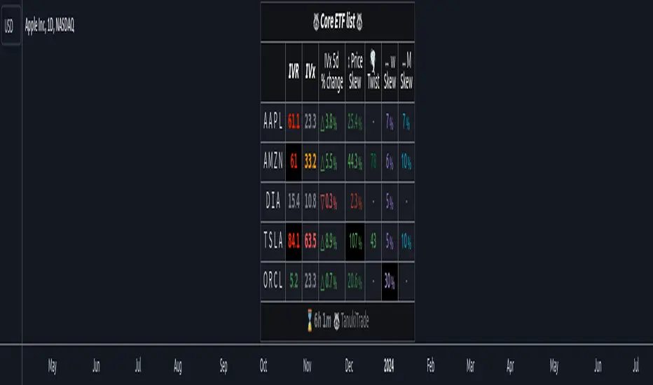
Asay (1982) Margined Futures Option Pricing Model [Loxx]Asay (1982) Margined Futures Option Pricing Model is an adaptation of the Black-Scholes-Merton Option Pricing Model including Analytical Greeks and implied volatility calculations. The following information is an excerpt from Espen Gaarder Haug's book "Option Pricing Formulas". This version is to price Options on Futures where premium is fully margined. This means the Risk-free Rate, dividend, and cost to carry are all zero. The options sensitivities (Greeks) are the partial derivatives of the Black-Scholes-Merton ( BSM ) formula. Analytical Greeks for our purposes here are broken down into various categories:
Delta Greeks: Delta, DDeltaDvol, Elasticity
Gamma Greeks: Gamma, GammaP, DGammaDvol, Speed
Vega Greeks: Vega , DVegaDvol/Vomma, VegaP
Theta Greeks: Theta
Probability Greeks: StrikeDelta, Risk Neutral Density
(See the code for more details)
Black-Scholes-Merton Option Pricing
The Black-Scholes-Merton model can be "generalized" by incorporating a cost-of-carry rate b. This model can be used to price European options on stocks, stocks paying a continuous dividend yield, options on futures , and currency options:
c = S * e^((b - r) * T) * N(d1) - X * e^(-r * T) * N(d2)
p = X * e^(-r * T) * N(-d2) - S * e^((b - r) * T) * N(-d1)
where
d1 = (log(S / X) + (b + v^2 / 2) * T) / (v * T^0.5)
d2 = d1 - v * T^0.5
b = r ... gives the Black and Scholes (1973) stock option model.
b = r — q ... gives the Merton (1973) stock option model with continuous dividend yield q.
b = 0 ... gives the Black (1976) futures option model.
b = 0 and r = 0 ... gives the Asay (1982) margined futures option model. <== this is the one used for this indicator!
b = r — rf ... gives the Garman and Kohlhagen (1983) currency option model.
Inputs
S = Stock price.
X = Strike price of option.
T = Time to expiration in years.
r = Risk-free rate
d = dividend yield
v = Volatility of the underlying asset price
cnd (x) = The cumulative normal distribution function
nd(x) = The standard normal density function
convertingToCCRate(r, cmp ) = Rate compounder
gImpliedVolatilityNR(string CallPutFlag, float S, float x, float T, float r, float b, float cm , float epsilon) = Implied volatility via Newton Raphson
gBlackScholesImpVolBisection(string CallPutFlag, float S, float x, float T, float r, float b, float cm ) = implied volatility via bisection
Implied Volatility: The Bisection Method
The Newton-Raphson method requires knowledge of the partial derivative of the option pricing formula with respect to volatility ( vega ) when searching for the implied volatility . For some options (exotic and American options in particular), vega is not known analytically. The bisection method is an even simpler method to estimate implied volatility when vega is unknown. The bisection method requires two initial volatility estimates (seed values):
1. A "low" estimate of the implied volatility , al, corresponding to an option value, CL
2. A "high" volatility estimate, aH, corresponding to an option value, CH
The option market price, Cm , lies between CL and cH . The bisection estimate is given as the linear interpolation between the two estimates:
v(i + 1) = v(L) + (c(m) - c(L)) * (v(H) - v(L)) / (c(H) - c(L))
Replace v(L) with v(i + 1) if c(v(i + 1)) < c(m), or else replace v(H) with v(i + 1) if c(v(i + 1)) > c(m) until |c(m) - c(v(i + 1))| <= E, at which point v(i + 1) is the implied volatility and E is the desired degree of accuracy.
Implied Volatility: Newton-Raphson Method
The Newton-Raphson method is an efficient way to find the implied volatility of an option contract. It is nothing more than a simple iteration technique for solving one-dimensional nonlinear equations (any introductory textbook in calculus will offer an intuitive explanation). The method seldom uses more than two to three iterations before it converges to the implied volatility . Let
v(i + 1) = v(i) + (c(v(i)) - c(m)) / (dc / dv (i))
until |c(m) - c(v(i + 1))| <= E at which point v(i + 1) is the implied volatility , E is the desired degree of accuracy, c(m) is the market price of the option, and dc/ dv (i) is the vega of the option evaluaated at v(i) (the sensitivity of the option value for a small change in volatility ).
Things to know
Only works on the daily timeframe and for the current source price.
You can adjust the text size to fit the screen
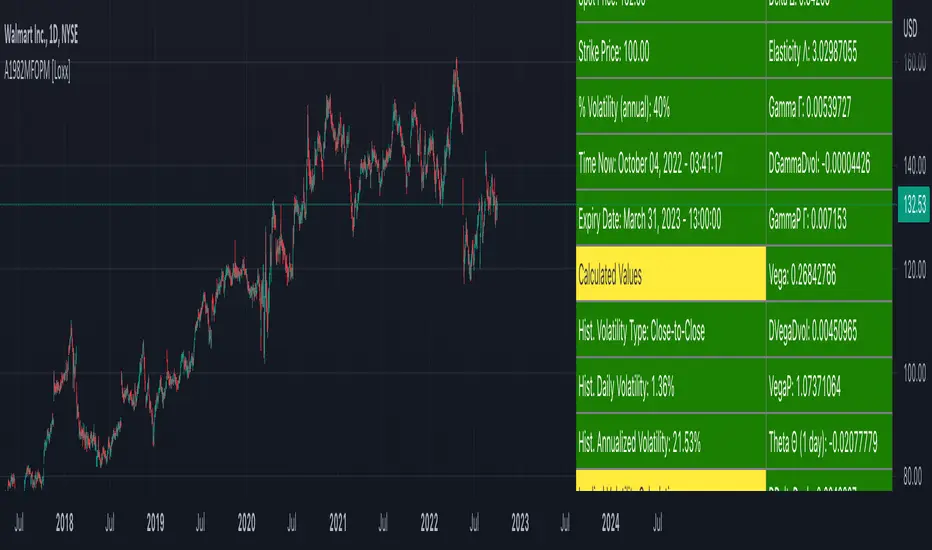
Black-76 Options on Futures [Loxx]Black-76 Options on Futures is an adaptation of the Black-Scholes-Merton Option Pricing Model including Analytical Greeks and implied volatility calculations. The following information is an excerpt from Espen Gaarder Haug's book "Option Pricing Formulas". This version is to price Options on Futures. The options sensitivities (Greeks) are the partial derivatives of the Black-Scholes-Merton ( BSM ) formula. Analytical Greeks for our purposes here are broken down into various categories:
Delta Greeks: Delta, DDeltaDvol, Elasticity
Gamma Greeks: Gamma, GammaP, DGammaDvol, Speed
Vega Greeks: Vega , DVegaDvol/Vomma, VegaP
Theta Greeks: Theta
Rate/Carry Greeks: Rho futures option
Probability Greeks: StrikeDelta, Risk Neutral Density
(See the code for more details)
Black-Scholes-Merton Option Pricing
The Black-Scholes-Merton model can be "generalized" by incorporating a cost-of-carry rate b. This model can be used to price European options on stocks, stocks paying a continuous dividend yield, options on futures , and currency options:
c = S * e^((b - r) * T) * N(d1) - X * e^(-r * T) * N(d2)
p = X * e^(-r * T) * N(-d2) - S * e^((b - r) * T) * N(-d1)
where
d1 = (log(S / X) + (b + v^2 / 2) * T) / (v * T^0.5)
d2 = d1 - v * T^0.5
b = r ... gives the Black and Scholes (1973) stock option model.
b = r — q ... gives the Merton (1973) stock option model with continuous dividend yield q.
b = 0 ... gives the Black (1976) futures option model. <== this is the one used for this indicator!
b = 0 and r = 0 ... gives the Asay (1982) margined futures option model.
b = r — rf ... gives the Garman and Kohlhagen (1983) currency option model.
Inputs
S = Stock price.
X = Strike price of option.
T = Time to expiration in years.
r = Risk-free rate
d = dividend yield
v = Volatility of the underlying asset price
cnd (x) = The cumulative normal distribution function
nd(x) = The standard normal density function
convertingToCCRate(r, cmp ) = Rate compounder
gImpliedVolatilityNR(string CallPutFlag, float S, float x, float T, float r, float b, float cm , float epsilon) = Implied volatility via Newton Raphson
gBlackScholesImpVolBisection(string CallPutFlag, float S, float x, float T, float r, float b, float cm ) = implied volatility via bisection
Implied Volatility: The Bisection Method
The Newton-Raphson method requires knowledge of the partial derivative of the option pricing formula with respect to volatility ( vega ) when searching for the implied volatility . For some options (exotic and American options in particular), vega is not known analytically. The bisection method is an even simpler method to estimate implied volatility when vega is unknown. The bisection method requires two initial volatility estimates (seed values):
1. A "low" estimate of the implied volatility , al, corresponding to an option value, CL
2. A "high" volatility estimate, aH, corresponding to an option value, CH
The option market price, Cm , lies between CL and cH . The bisection estimate is given as the linear interpolation between the two estimates:
v(i + 1) = v(L) + (c(m) - c(L)) * (v(H) - v(L)) / (c(H) - c(L))
Replace v(L) with v(i + 1) if c(v(i + 1)) < c(m), or else replace v(H) with v(i + 1) if c(v(i + 1)) > c(m) until |c(m) - c(v(i + 1))| <= E, at which point v(i + 1) is the implied volatility and E is the desired degree of accuracy.
Implied Volatility: Newton-Raphson Method
The Newton-Raphson method is an efficient way to find the implied volatility of an option contract. It is nothing more than a simple iteration technique for solving one-dimensional nonlinear equations (any introductory textbook in calculus will offer an intuitive explanation). The method seldom uses more than two to three iterations before it converges to the implied volatility . Let
v(i + 1) = v(i) + (c(v(i)) - c(m)) / (dc / dv (i))
until |c(m) - c(v(i + 1))| <= E at which point v(i + 1) is the implied volatility , E is the desired degree of accuracy, c(m) is the market price of the option, and dc/ dv (i) is the vega of the option evaluaated at v(i) (the sensitivity of the option value for a small change in volatility ).
Things to know
Only works on the daily timeframe and for the current source price.
You can adjust the text size to fit the screen
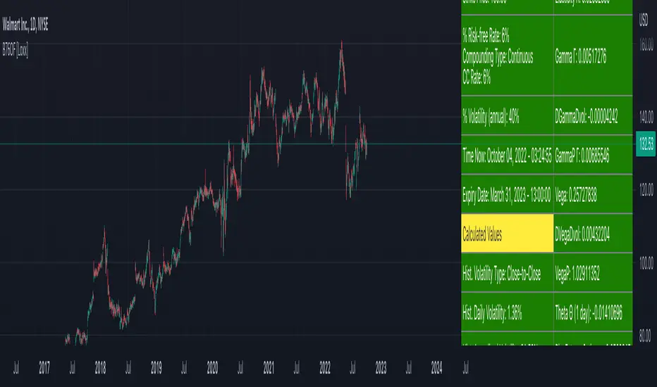
Garman and Kohlhagen (1983) for Currency Options [Loxx]Garman and Kohlhagen (1983) for Currency Options is an adaptation of the Black-Scholes-Merton Option Pricing Model including Analytical Greeks and implied volatility calculations. The following information is an excerpt from Espen Gaarder Haug's book "Option Pricing Formulas". This version of BSMOPM is to price Currency Options. The options sensitivities (Greeks) are the partial derivatives of the Black-Scholes-Merton ( BSM ) formula. Analytical Greeks for our purposes here are broken down into various categories:
Delta Greeks: Delta, DDeltaDvol, Elasticity
Gamma Greeks: Gamma, GammaP, DGammaDSpot/speed, DGammaDvol/Zomma
Vega Greeks: Vega , DVegaDvol/Vomma, VegaP, Speed
Theta Greeks: Theta
Rate/Carry Greeks: Rho, Rho futures option, Carry Rho, Phi/Rho2
Probability Greeks: StrikeDelta, Risk Neutral Density
(See the code for more details)
Black-Scholes-Merton Option Pricing for Currency Options
The Garman and Kohlhagen (1983) modified Black-Scholes model can be used to price European currency options; see also Grabbe (1983). The model is mathematically equivalent to the Merton (1973) model presented earlier. The only difference is that the dividend yield is replaced by the risk-free rate of the foreign currency rf:
c = S * e^(-rf * T) * N(d1) - X * e^(-r * T) * N(d2)
p = X * e^(-r * T) * N(-d2) - S * e^(-rf * T) * N(-d1)
where
d1 = (log(S / X) + (r - rf + v^2 / 2) * T) / (v * T^0.5)
d2 = d1 - v * T^0.5
For more information on currency options, see DeRosa (2000)
Inputs
S = Stock price.
X = Strike price of option.
T = Time to expiration in years.
r = Risk-free rate
rf = Risk-free rate of the foreign currency
v = Volatility of the underlying asset price
cnd (x) = The cumulative normal distribution function
nd(x) = The standard normal density function
convertingToCCRate(r, cmp ) = Rate compounder
gImpliedVolatilityNR(string CallPutFlag, float S, float x, float T, float r, float b, float cm , float epsilon) = Implied volatility via Newton Raphson
gBlackScholesImpVolBisection(string CallPutFlag, float S, float x, float T, float r, float b, float cm ) = implied volatility via bisection
Implied Volatility: The Bisection Method
The Newton-Raphson method requires knowledge of the partial derivative of the option pricing formula with respect to volatility ( vega ) when searching for the implied volatility . For some options (exotic and American options in particular), vega is not known analytically. The bisection method is an even simpler method to estimate implied volatility when vega is unknown. The bisection method requires two initial volatility estimates (seed values):
1. A "low" estimate of the implied volatility , al, corresponding to an option value, CL
2. A "high" volatility estimate, aH, corresponding to an option value, CH
The option market price, Cm , lies between CL and cH . The bisection estimate is given as the linear interpolation between the two estimates:
v(i + 1) = v(L) + (c(m) - c(L)) * (v(H) - v(L)) / (c(H) - c(L))
Replace v(L) with v(i + 1) if c(v(i + 1)) < c(m), or else replace v(H) with v(i + 1) if c(v(i + 1)) > c(m) until |c(m) - c(v(i + 1))| <= E, at which point v(i + 1) is the implied volatility and E is the desired degree of accuracy.
Implied Volatility: Newton-Raphson Method
The Newton-Raphson method is an efficient way to find the implied volatility of an option contract. It is nothing more than a simple iteration technique for solving one-dimensional nonlinear equations (any introductory textbook in calculus will offer an intuitive explanation). The method seldom uses more than two to three iterations before it converges to the implied volatility . Let
v(i + 1) = v(i) + (c(v(i)) - c(m)) / (dc / dv (i))
until |c(m) - c(v(i + 1))| <= E at which point v(i + 1) is the implied volatility , E is the desired degree of accuracy, c(m) is the market price of the option, and dc/ dv (i) is the vega of the option evaluaated at v(i) (the sensitivity of the option value for a small change in volatility ).
Things to know
Only works on the daily timeframe and for the current source price.
You can adjust the text size to fit the screen
Related indicators:
BSM OPM 1973 w/ Continuous Dividend Yield
Black-Scholes 1973 OPM on Non-Dividend Paying Stocks
Generalized Black-Scholes-Merton w/ Analytical Greeks
Generalized Black-Scholes-Merton Option Pricing Formula
Sprenkle 1964 Option Pricing Model w/ Num. Greeks
Modified Bachelier Option Pricing Model w/ Num. Greeks
Bachelier 1900 Option Pricing Model w/ Numerical Greeks

Black-Scholes 1973 OPM on Non-Dividend Paying Stocks [Loxx]Black-Scholes 1973 OPM on Non-Dividend Paying Stocks is an adaptation of the Black-Scholes-Merton Option Pricing Model including Analytical Greeks and implied volatility calculations. Making b equal to r yields the BSM model where dividends are not considered. The following information is an excerpt from Espen Gaarder Haug's book "Option Pricing Formulas". The options sensitivities (Greeks) are the partial derivatives of the Black-Scholes-Merton ( BSM ) formula. For our purposes here are, Analytical Greeks are broken down into various categories:
Delta Greeks: Delta, DDeltaDvol, Elasticity
Gamma Greeks: Gamma, GammaP, DGammaDSpot/speed, DGammaDvol/Zomma
Vega Greeks: Vega , DVegaDvol/Vomma, VegaP
Theta Greeks: Theta
Rate/Carry Greeks: Rho
Probability Greeks: StrikeDelta, Risk Neutral Density
(See the code for more details)
Black-Scholes-Merton Option Pricing
The BSM formula and its binomial counterpart may easily be the most used "probability model/tool" in everyday use — even if we con- sider all other scientific disciplines. Literally tens of thousands of people, including traders, market makers, and salespeople, use option formulas several times a day. Hardly any other area has seen such dramatic growth as the options and derivatives businesses. In this chapter we look at the various versions of the basic option formula. In 1997 Myron Scholes and Robert Merton were awarded the Nobel Prize (The Bank of Sweden Prize in Economic Sciences in Memory of Alfred Nobel). Unfortunately, Fischer Black died of cancer in 1995 before he also would have received the prize.
It is worth mentioning that it was not the option formula itself that Myron Scholes and Robert Merton were awarded the Nobel Prize for, the formula was actually already invented, but rather for the way they derived it — the replicating portfolio argument, continuous- time dynamic delta hedging, as well as making the formula consistent with the capital asset pricing model (CAPM). The continuous dynamic replication argument is unfortunately far from robust. The popularity among traders for using option formulas heavily relies on hedging options with options and on the top of this dynamic delta hedging, see Higgins (1902), Nelson (1904), Mello and Neuhaus (1998), Derman and Taleb (2005), as well as Haug (2006) for more details on this topic. In any case, this book is about option formulas and not so much about how to derive them.
Provided here are the various versions of the Black-Scholes-Merton formula presented in the literature. All formulas in this section are originally derived based on the underlying asset S follows a geometric Brownian motion
dS = mu * S * dt + v * S * dz
where t is the expected instantaneous rate of return on the underlying asset, a is the instantaneous volatility of the rate of return, and dz is a Wiener process.
The formula derived by Black and Scholes (1973) can be used to value a European option on a stock that does not pay dividends before the option's expiration date. Letting c and p denote the price of European call and put options, respectively, the formula states that
c = S * N(d1) - X * e^(-r * T) * N(d2)
p = X * e^(-r * T) * N(d2) - S * N(d1)
where
d1 = (log(S / X) + (r + v^2 / 2) * T) / (v * T^0.5)
d2 = (log(S / X) + (r - v^2 / 2) * T) / (v * T^0.5) = d1 - v * T^0.5
**This version of the Black-Scholes formula can also be used to price American call options on a non-dividend-paying stock, since it will never be optimal to exercise the option before expiration.**
Inputs
S = Stock price.
X = Strike price of option.
T = Time to expiration in years.
r = Risk-free rate
b = Cost of carry
v = Volatility of the underlying asset price
cnd (x) = The cumulative normal distribution function
nd(x) = The standard normal density function
convertingToCCRate(r, cmp ) = Rate compounder
gImpliedVolatilityNR(string CallPutFlag, float S, float x, float T, float r, float b, float cm , float epsilon) = Implied volatility via Newton Raphson
gBlackScholesImpVolBisection(string CallPutFlag, float S, float x, float T, float r, float b, float cm ) = implied volatility via bisection
Implied Volatility: The Bisection Method
The Newton-Raphson method requires knowledge of the partial derivative of the option pricing formula with respect to volatility ( vega ) when searching for the implied volatility . For some options (exotic and American options in particular), vega is not known analytically. The bisection method is an even simpler method to estimate implied volatility when vega is unknown. The bisection method requires two initial volatility estimates (seed values):
1. A "low" estimate of the implied volatility , al, corresponding to an option value, CL
2. A "high" volatility estimate, aH, corresponding to an option value, CH
The option market price, Cm , lies between CL and cH . The bisection estimate is given as the linear interpolation between the two estimates:
v(i + 1) = v(L) + (c(m) - c(L)) * (v(H) - v(L)) / (c(H) - c(L))
Replace v(L) with v(i + 1) if c(v(i + 1)) < c(m), or else replace v(H) with v(i + 1) if c(v(i + 1)) > c(m) until |c(m) - c(v(i + 1))| <= E, at which point v(i + 1) is the implied volatility and E is the desired degree of accuracy.
Implied Volatility: Newton-Raphson Method
The Newton-Raphson method is an efficient way to find the implied volatility of an option contract. It is nothing more than a simple iteration technique for solving one-dimensional nonlinear equations (any introductory textbook in calculus will offer an intuitive explanation). The method seldom uses more than two to three iterations before it converges to the implied volatility . Let
v(i + 1) = v(i) + (c(v(i)) - c(m)) / (dc / dv (i))
until |c(m) - c(v(i + 1))| <= E at which point v(i + 1) is the implied volatility , E is the desired degree of accuracy, c(m) is the market price of the option, and dc/ dv (i) is the vega of the option evaluaated at v(i) (the sensitivity of the option value for a small change in volatility ).
Things to know
Only works on the daily timeframe and for the current source price.
You can adjust the text size to fit the screen

Generalized Black-Scholes-Merton Option Pricing Formula [Loxx]Generalized Black-Scholes-Merton Option Pricing Formula is an adaptation of the Black-Scholes-Merton Option Pricing Model including Numerical Greeks aka "Option Sensitivities" and implied volatility calculations. The following information is an excerpt from Espen Gaarder Haug's book "Option Pricing Formulas".
Black-Scholes-Merton Option Pricing
The BSM formula and its binomial counterpart may easily be the most used "probability model/tool" in everyday use — even if we con- sider all other scientific disciplines. Literally tens of thousands of people, including traders, market makers, and salespeople, use option formulas several times a day. Hardly any other area has seen such dramatic growth as the options and derivatives businesses. In this chapter we look at the various versions of the basic option formula. In 1997 Myron Scholes and Robert Merton were awarded the Nobel Prize (The Bank of Sweden Prize in Economic Sciences in Memory of Alfred Nobel). Unfortunately, Fischer Black died of cancer in 1995 before he also would have received the prize.
It is worth mentioning that it was not the option formula itself that Myron Scholes and Robert Merton were awarded the Nobel Prize for, the formula was actually already invented, but rather for the way they derived it — the replicating portfolio argument, continuous- time dynamic delta hedging, as well as making the formula consistent with the capital asset pricing model (CAPM). The continuous dynamic replication argument is unfortunately far from robust. The popularity among traders for using option formulas heavily relies on hedging options with options and on the top of this dynamic delta hedging, see Higgins (1902), Nelson (1904), Mello and Neuhaus (1998), Derman and Taleb (2005), as well as Haug (2006) for more details on this topic. In any case, this book is about option formulas and not so much about how to derive them.
Provided here are the various versions of the Black-Scholes-Merton formula presented in the literature. All formulas in this section are originally derived based on the underlying asset S follows a geometric Brownian motion
dS = mu * S * dt + v * S * dz
where t is the expected instantaneous rate of return on the underlying asset, a is the instantaneous volatility of the rate of return, and dz is a Wiener process.
The formula derived by Black and Scholes (1973) can be used to value a European option on a stock that does not pay dividends before the option's expiration date. Letting c and p denote the price of European call and put options, respectively, the formula states that
c = S * N(d1) - X * e^(-r * T) * N(d2)
p = X * e^(-r * T) * N(d2) - S * N(d1)
where
d1 = (log(S / X) + (r + v^2 / 2) * T) / (v * T^0.5)
d2 = (log(S / X) + (r - v^2 / 2) * T) / (v * T^0.5) = d1 - v * T^0.5
Inputs
S = Stock price.
X = Strike price of option.
T = Time to expiration in years.
r = Risk-free rate
b = Cost of carry
v = Volatility of the underlying asset price
cnd (x) = The cumulative normal distribution function
nd(x) = The standard normal density function
convertingToCCRate(r, cmp ) = Rate compounder
gImpliedVolatilityNR(string CallPutFlag, float S, float x, float T, float r, float b, float cm, float epsilon) = Implied volatility via Newton Raphson
gBlackScholesImpVolBisection(string CallPutFlag, float S, float x, float T, float r, float b, float cm) = implied volatility via bisection
Implied Volatility: The Bisection Method
The Newton-Raphson method requires knowledge of the partial derivative of the option pricing formula with respect to volatility (vega) when searching for the implied volatility. For some options (exotic and American options in particular), vega is not known analytically. The bisection method is an even simpler method to estimate implied volatility when vega is unknown. The bisection method requires two initial volatility estimates (seed values):
1. A "low" estimate of the implied volatility, al, corresponding to an option value, CL
2. A "high" volatility estimate, aH, corresponding to an option value, CH
The option market price, Cm, lies between CL and cH. The bisection estimate is given as the linear interpolation between the two estimates:
v(i + 1) = v(L) + (c(m) - c(L)) * (v(H) - v(L)) / (c(H) - c(L))
Replace v(L) with v(i + 1) if c(v(i + 1)) < c(m), or else replace v(H) with v(i + 1) if c(v(i + 1)) > c(m) until |c(m) - c(v(i + 1))| <= E, at which point v(i + 1) is the implied volatility and E is the desired degree of accuracy.
Implied Volatility: Newton-Raphson Method
The Newton-Raphson method is an efficient way to find the implied volatility of an option contract. It is nothing more than a simple iteration technique for solving one-dimensional nonlinear equations (any introductory textbook in calculus will offer an intuitive explanation). The method seldom uses more than two to three iterations before it converges to the implied volatility. Let
v(i + 1) = v(i) + (c(v(i)) - c(m)) / (dc / dv(i))
until |c(m) - c(v(i + 1))| <= E at which point v(i + 1) is the implied volatility, E is the desired degree of accuracy, c(m) is the market price of the option, and dc/dv(i) is the vega of the option evaluaated at v(i) (the sensitivity of the option value for a small change in volatility).
Numerical Greeks or Greeks by Finite Difference
Analytical Greeks are the standard approach to estimating Delta, Gamma etc... That is what we typically use when we can derive from closed form solutions. Normally, these are well-defined and available in text books. Previously, we relied on closed form solutions for the call or put formulae differentiated with respect to the Black Scholes parameters. When Greeks formulae are difficult to develop or tease out, we can alternatively employ numerical Greeks - sometimes referred to finite difference approximations. A key advantage of numerical Greeks relates to their estimation independent of deriving mathematical Greeks. This could be important when we examine American options where there may not technically exist an exact closed form solution that is straightforward to work with. (via VinegarHill FinanceLabs)
Things to know
Only works on the daily timeframe and for the current source price.
You can adjust the text size to fit the screen
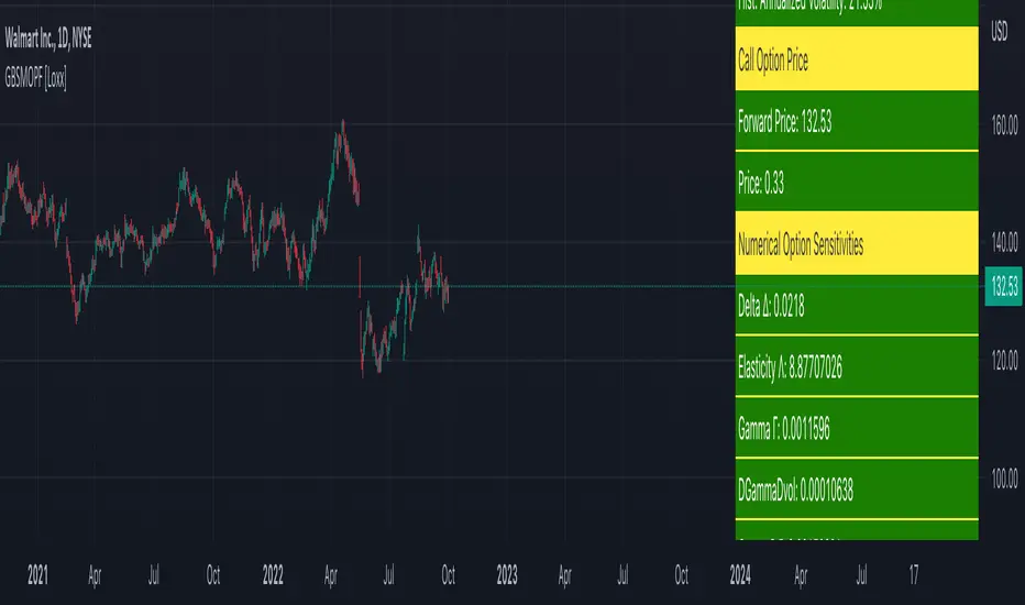
Options Oscillator [Lite] IVRank, IVx, Call/Put Volatility Skew The first TradingView indicator that provides REAL IVRank, IVx, and CALL/PUT skew data based on REAL option chain for 5 U.S. market symbols.
🔃 Auto-Updating Option Metrics without refresh!
🍒 Developed and maintained by option traders for option traders.
📈 Specifically designed for TradingView users who trade options.
🔶 Ticker Information:
This 'Lite' indicator is currently only available for 5 liquid U.S. market smbols : NASDAQ:TSLA AMEX:DIA NASDAQ:AAPL NASDAQ:AMZN and NYSE:ORCL
🔶 How does the indicator work and why is it unique?
This Pine Script indicator is a complex tool designed to provide various option metrics and visualization tools for options market traders. The indicator extracts raw options data from an external data provider (ORATS), processes and refines the delayed data package using pineseed, and sends it to TradingView, visualizing the data using specific formulas (see detailed below) or interpolated values (e.g., delta distances). This method of incorporating options data into a visualization framework is unique and entirely innovative on TradingView.
The indicator aims to offer a comprehensive view of the current state of options for the implemented instruments, including implied volatility (IV), IV rank (IVR), options skew, and expected market movements, which are objectively measured as detailed below.
The options metrics we display may be familiar to options traders from various major brokerage platforms such as TastyTrade, IBKR, TOS, Tradier, TD Ameritrade, Schwab, etc.
🟨 The following data is displayed in the oscillator 🟨
We use Tastytrade formulas, so our numbers mostly align with theirs!
🔶 𝗜𝗩𝗥𝗮𝗻𝗸
The Implied Volatility Rank (IVR) helps options traders assess the current level of implied volatility (IV) in comparison to the past 52 weeks. IVR is a useful metric to determine whether options are relatively cheap or expensive. This can guide traders on whether to buy or sell options.
IV Rank formula = (current IV - 52 week IV low) / (52 week IV high - 52 week IV low)
IVRank is default blue and you can adjust their settings:
🔶 𝗜𝗩𝘅 𝗮𝘃𝗴
The implied volatility (IVx) shown in the option chain is calculated like the VIX. The Cboe uses standard and weekly SPX options to measure expected S&P 500 volatility. A similar method is used for calculating IVx for each expiration cycle.
We aggregate the IVx values for the 35-70 day monthly expiration cycle, and use that value in the oscillator and info panel.
We always display which expiration the IVx values are averaged for when you hover over the IVx cell.
IVx main color is purple, but you can change the settings:
🔹IVx 5 days change %
We are also displaying the five-day change of the IV Index (IVx value). The IV Index 5-Day Change column provides quick insight into recent expansions or decreases in implied volatility over the last five trading days.
Traders who expect the value of options to decrease might view a decrease in IVX as a positive signal. Strategies such as Strangle and Ratio Spread can benefit from this decrease.
On the other hand, traders anticipating further increases in IVX will focus on the rising IVX values. Strategies like Calendar Spread or Diagonal Spread can take advantage of increasing implied volatility.
This indicator helps traders quickly assess changes in implied volatility, enabling them to make informed decisions based on their trading strategies and market expectations.
Important Note:
The IVx value alone does not provide sufficient context. There are stocks that inherently exhibit high IVx values. Therefore, it is crucial to consider IVx in conjunction with the Implied Volatility Rank (IVR), which measures the IVx relative to its own historical values. This combined view helps in accurately assessing the significance of the IVx in relation to the specific stock's typical volatility behavior.
This indicator offers traders a comprehensive view of implied volatility, assisting them in making informed decisions by highlighting both the absolute and relative volatility measures.
🔶 𝗖𝗔𝗟𝗟/𝗣𝗨𝗧 𝗣𝗿𝗶𝗰𝗶𝗻𝗴 𝗦𝗸𝗲𝘄 𝗵𝗶𝘀𝘁𝗼𝗴𝗿𝗮𝗺
At TanukiTrade, Vertical Pricing Skew refers to the difference in pricing between put and call options with the same expiration date at the same distance (at tastytrade binary expected move). We analyze this skew to understand market sentiment. This is the same formula used by TastyTrade for calculations.
We calculate the interpolated strike price based on the expected move, taking into account the neighboring option prices and their distances. This allows us to accurately determine whether the CALL or PUT options are more expensive.
🔹 What Causes Pricing Skew? The Theory Behind It
The asymmetric pricing of PUT and CALL options is driven by the natural dynamics of the market. The theory is that when CALL options are more expensive than PUT options at the same distance from the current spot price, market participants are buying CALLs and selling PUTs, expecting a faster upward movement compared to a downward one .
In the case of PUT skew, it's the opposite: participants are buying PUTs and selling CALLs , as they expect a potential downward move to happen more quickly than an upward one.
An options trader can take advantage of this phenomenon by leveraging PUT pricing skew. For example, if they have a bullish outlook and both IVR and IVx are high and IV started decreasing, they can capitalize on this PUT skew with strategies like a jade lizard, broken wing butterfly, or short put.
🔴 PUT Skew 🔴
Put options are more expensive than call options, indicating the market expects a faster downward move (▽). This alone doesn't indicate which way the market will move (because nobody knows that), but the options chain pricing suggests that if the market moves downward, it could do so faster in velocity compared to a potential upward movement.
🔹 SPY PUT SKEW example:
If AMEX:SPY PUT option prices are 46% higher than CALLs at the same distance for the optimal next monthly expiry (DTE). This alone doesn't indicate which way the market will move (because nobody knows that), but the options chain pricing suggests that if the market moves downward, it could do so 46% faster in velocity compared to a potential upward movement
🟢 CALL Skew 🟢
Call options are more expensive than put options, indicating the market expects a faster upward move (△). This alone doesn't indicate which way the market will move (because nobody knows that), but the options chain pricing suggests that if the market moves upward, it could do so faster in velocity compared to a potential downward movement.
🔹 INTC CALL SKEW example:
If NASDAQ:INTC CALL option prices are 49% higher than PUTs at the same distance for the optimal next monthly expiry (DTE). This alone doesn't indicate which way the market will move (because nobody knows that), but the options chain pricing suggests that if the market moves upward, it could do so 49% faster in velocity compared to a potential downward movement .
🔶 USAGE example:
The script is compatible with our other options indicators.
For example: Since the main metrics are already available in this Options Oscillator, you can hide the main IVR panel of our Options Overlay indicator, freeing up more space on the chart. The following image shows this:
🔶 ADDITIONAL IMPORTANT COMMENTS
🔹 Historical Data:
Yes, we only using historical internal metrics dating back to 2024-07-01, when the TanukiTrade options brand launched. For now, we're using these, but we may expand the historical data in the future.
🔹 What distance does the indicator use to measure the call/put pricing skew?:
It is important to highlight that this oscillator displays the call/put pricing skew changes for the next optimal monthly expiration on a histogram.
The Binary Expected Move distance is calculated using the TastyTrade method for the next optimal monthly expiration: Formula = (ATM straddle price x 0.6) + (1st OTM strangle price x 0.3) + (2nd OTM strangle price x 0.1)
We interpolate the exact difference based on the neighboring strikes at the binary expected move distance using the TastyTrade method, and compare the interpolated call and put prices at this specific point.
🔹 - Why is there a slight difference between the displayed data and my live brokerage data?
There are two reasons for this, and one is beyond our control.
◎ Option-data update frequency:
According to TradingView's regulations and guidelines, we can update external data a maximum of 5 times per day. We strive to use these updates in the most optimal way:
(1st update) 15 minutes after U.S. market open
(2nd, 3rd, 4th updates) 1.5–3 hours during U.S. market open hours
(5th update) 10 minutes before U.S. market close.
You don’t need to refresh your window, our last refreshed data-pack is always automatically applied to your indicator, and you can see the time elapsed since the last update at the bottom of the corner on daily TF.
◎ Brokerage Calculation Differences:
Every brokerage has slight differences in how they calculate metrics like IV and IVx. If you open three windows for TOS, TastyTrade, and IBKR side by side, you will notice that the values are minimally different. We had to choose a standard, so we use the formulas and mathematical models described by TastyTrade when analyzing the options chain and drawing conclusions.
🔹 - EOD data:
The indicator always displays end-of-day (EOD) data for IVR, IV, and CALL/PUT pricing skew. During trading hours, it shows the current values for the ongoing day with each update, and at market close, these values become final. From that point on, the data is considered EOD, provided the day confirms as a closed daily candle.
🔹 - U.S. market only:
Since we only deal with liquid option chains: this option indicator only works for the USA options market and do not include future contracts; we have implemented each selected symbol individually.
Disclaimer:
Our option indicator uses approximately 15min-3 hour delayed option market snapshot data to calculate the main option metrics. Exact realtime option contract prices are never displayed; only derived metrics and interpolated delta are shown to ensure accurate and consistent visualization. Due to the above, this indicator can only be used for decision support; exclusive decisions cannot be made based on this indicator. We reserve the right to make errors.This indicator is designed for options traders who understand what they are doing. It assumes that they are familiar with options and can make well-informed, independent decisions. We work with public data and are not a data provider; therefore, we do not bear any financial or other liability.